Scheduling for heavy-tailed and light-tailed workloads in
queueing systems
Thesis by
Jayakrishnan U. Nair
In Partial Fulfillment of the Requirements for the Degree of
Doctor of Philosophy
California Institute of Technology Pasadena, California
2012
c
2012
iii
This thesis is dedicated to
my wife Sushree,
whose companionship makes my life complete,
and my parents,
v
Acknowledgements
I have had a very memorable five years as a graduate student at Caltech, and it is with great pleasure that I acknowledge the people who made this possible.
First, I thank my advisor Adam Wierman for his guidance over the years, on research matters, and beyond. No Ph.D. career is without the occasional roadblock, and Adam’s encouragement has been instrumental in helping me navigate around mine. Adam’s boundless excitement about research, his ability to communicate complex ideas cleanly and effectively, and his knack of always seeing the big picture, without being encum-bered by the details, have been a constant source of inspiration for me. It’s been an honor working with you, Adam!
I am also very grateful to my advisor Steven Low for his support and advice throughout my graduate study. Steven guided my first research endeavors at Caltech, and got me interested in heavy-tailed phenomena as a theme for my thesis. Thanks, Steven! I would like to thank my thesis committee members: Mani Chandy, Babak Hassibi, and Tracey Ho, for their valuable feedback on this thesis.
I have had the chance to work with some brilliant collaborators as a graduate student, I am grateful to them for the opportunity. Collaborations with Bert Zwart, Sachin Adlakha, Krishna Jagannathan, and Lachlan Andrew have been highly rewarding. I also thank Bert for hosting me at CWI in the Netherlands on two occasions. I am thankful to Prof. Borkar for hosting me at the Tata Institute of Fundamental Research in India over the summer of 2010.
I have benefited immensely from the research environment in the RSRG group. I thank the group mem-bers — working alongside you guys has been very inspiring. I would also like to thank the exceptionally helpful administrative staff in Annenberg, especially Sydney Garstang.
Moving to life outside academia, I would like to acknowledge the desi gang at Caltech for some wonderful times. I specially wish to thank Rangoli, Krishna, Prabha, Varun, Uday, Shweta, and Mayank.
vii
Abstract
In much of classical queueing theory, workloads are assumed to be light-tailed, with job sizes being described using exponential or phase type distributions. However, over the past two decades, studies have shown that several real-world workloads exhibit heavy-tailed characteristics. As a result, there has been a strong interest in studying queues with heavy-tailed workloads. So at this stage, there is a large body of literature on queues with light-tailed workloads, and a large body of literature on queues with heavy-tailed workloads. However, heavy-tailed workloads and light-tailed workloads differ considerably in their behavior, and these two types of workloads are rarely studied jointly.
In this thesis, we design scheduling policies for queueing systems, considering both heavy-tailed as well as light-tailed workloads. The motivation for this line of work is twofold. First, since real world workloads can be heavy-tailed or light-tailed, it is desirable to design schedulers that are robust in their performance to distributional assumptions on the workload. Second, there might be scenarios where a heavy-tailed and a light-tailed workload interact in a queueing system. In such cases, it is desirable to design schedulers that guarantee fairness in resource allocation for both workload types.
ix
Contents
Acknowledgements v
Abstract vii
1 Introduction 1
2 Heavy-tailed and light-tailed distributions 7
2.1 Heavy-tailed distributions . . . 7
2.1.1 Definition and examples . . . 7
2.1.2 Important subclasses of heavy-tailed distributions . . . 9
2.1.3 The catastrophe principle . . . 10
2.2 Light-tailed distributions . . . 11
2.2.1 Definition . . . 11
2.2.2 The conspiracy principle . . . 11
3 Server Failures and Recovery Mechanisms: The Impact on the Processing Time Tail 15 3.1 Motivation and summary . . . 15
3.2 Model and preliminaries . . . 16
3.2.1 Model . . . 16
3.2.2 Notation and preliminaries . . . 17
3.3 Completion time tail asymptotics . . . 19
3.3.1 Results . . . 20
3.3.2 Proofs of Theorems 5–7 . . . 21
3.4 Fragmentation to minimize the average completion time . . . 24
3.4.1 Optimal policy . . . 25
3.4.2 Simple blind policyx(l) = min{a, l} . . . 29
3.4.3 Tail asymptotics under policiesx∗anda. . . 30
Appendices 30
3.A Proof of Lemma 2 . . . 31
3.B Proof of Theorem 12: Tail asymptotics ofT∗(L) . . . 32
4 Tail-Robust Scheduling via Limited Processor Sharing 33 4.1 Introduction . . . 33
4.2 Preliminaries . . . 36
4.2.1 Model and notation . . . 36
4.2.2 Heavy-tailed and light-tailed distributions . . . 36
4.2.3 Related literature . . . 37
4.2.4 Busy period decay rate as a function of server speed . . . 38
4.3 Tail asymptotics under heavy-tailed job sizes . . . 39
4.4 Tail asymptotics under light-tailed job sizes . . . 40
4.4.1 Interpreting the decay rate under LPS-c . . . 41
4.4.2 Properties of the decay rate under LPS-c. . . 42
4.5 Designing LPS robustly . . . 44
4.6 Concluding remarks . . . 47
Appendices 47 4.A Proofs for results in Section 4.3 . . . 47
4.A.1 Upper bound . . . 48
4.A.2 Lower bound . . . 48
4.A.3 Proof of Theorem 13 . . . 51
4.B Proofs for results in Section 4.4 . . . 51
4.B.1 Proof of Theorem 14: Lower bound for the caseγ(B)∈(0,∞) . . . 52
4.B.2 Proof of Theorem 14: Upper bound for the caseγ(B)∈(0,∞) . . . 53
4.B.3 Proof of Theorem 14: The case ofγ(B) =∞ . . . 56
4.B.4 Proof of Lemma 11 . . . 56
4.B.5 Proof of Lemma 12 . . . 56
4.C Proof of Corollaries 2 and 3 in Section 4.5 . . . 57
5 When Heavy-Tailed and Light-Tailed Flows Compete: Response Time Tail Under Generalized Max-Weight Scheduling 59 5.1 Introduction . . . 59
5.2 Model and preliminaries . . . 61
5.2.1 System model . . . 61
xi
5.2.3 Notation and preliminaries . . . 64
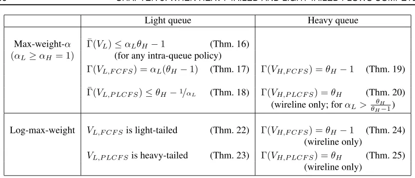
5.3 Summary of results . . . 65
5.3.1 Max-weight-αscheduling . . . 66
5.3.2 Log-max-weight scheduling . . . 67
5.4 Max-weight-αscheduling between queues . . . 68
5.4.1 The response time tail for the light queue . . . 69
5.4.2 The response time tail for the heavy queue . . . 73
5.5 Log-max-weight scheduling between queues . . . 77
5.5.1 The response time tail for the light queue . . . 79
5.5.2 The response time tail for the heavy queue . . . 81
5.6 Concluding remarks . . . 82
Appendices 83 5.A Proofs of Lemmas 23 and 24 . . . 83
5.B Technical lemmas . . . 84
5.C Proof of Theorem 18 . . . 85
5.D Proof of Lemma 25 . . . 88
5.E Proof of Theorem 22 . . . 89
5.E.1 Proof of Lemma 27 . . . 89
5.E.2 Proof of Lemma 28 . . . 91
5.F Proof of Theorem 23 . . . 93
xiii
List of Figures
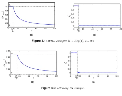
4.1 M/M/1 example:B∼Exp(1), ρ= 0.9 . . . 44
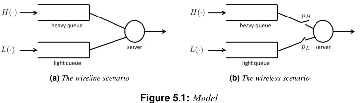
4.2 M/Erlang-2/1 example . . . 44
5.1 Model . . . 61
xv
List of Tables
Chapter 1
Introduction
In queueing systems, it is well known that variability in the incoming workload has a significant impact on the congestion experienced by incoming jobs. As a result, modeling workload variability is a key aspect of performance evaluation in queueing systems.
In classical queueing theory, variability in the workload is typically modeled via the class of phase-type distributions; most commonly, using the exponential distribution [17, 37]. The benefit of this modeling approach is that it enables the analysis of the queue using Markov chains. However, phase-type distributions are limited in the extent of variability they can capture. Specifically, all phase-type distributions are light-tailed.
However, over the past two decades, studies have shown that several real-life workloads exhibit extremely high variability, and are better modeled usingheavy-taileddistributions [4, 19, 29]. Empirical studies have also shown that internet traffic exhibits long range dependence and self similarity [8, 39]. The prevailing explanation for these properties is that they are caused by the heavy-tailed distribution of internet file sizes [18,30]. Consequently, there has been a considerable interest over the past two decades in analyzing queueing models with heavy-tailed workloads.
In general, one expects that certain real-world workloads are best described via light-tailed distributions, while others are best described using heavy-tailed distributions. However, there are fundamental differences in the behavior of heavy-tailed and light-tailed workloads. Specifically, this difference lies in the manner in which collections of heavy-tailed and light-tailed random variables cause rare events.
Collections of heavy-tailed random variables tend to obey thecatastrophe principle, which states that rare events occur most likely due to the smallest possible number of contributing factors. In queueing systems with heavy-tailed workloads, this principle manifests itself in the manner in which rare events such as large delays or backlogs occur: they occur most likely due to the arrival of one (or a few) large jobs into the system [11, 13, 68].
2 CHAPTER 1: INTRODUCTION
caused by a conspiracy involving a large number of jobs that are stochastically larger than usual, arriving at a stochastically faster rate than usual [2, 13].
The above dichotomy, which we elaborate on in greater detail in Chapter 2, creates a tension between scheduling for heavy-tailed and light-tailed workloads. In general, scheduling disciplines that work well under heavy-tailed workloads do not perform well under light-tailed workloads, and vice versa. This is particularly true when the performance metric under consideration involves the probability of rare events (see [13, 68]).
So at this stage, the literature understands how to schedule for good performance with light-tailed work-loads, as well as how to schedule for good performance with heavy-tailed workloads. However, these con-trasting workload types are rarely studied jointly. In this thesis, we design scheduling policies jointly for heavy-tailed and light-tailed workloads.
One key motivation for this line of work is robustness. Since real world workloads might be heavy-tailed or light-tailed, it is desirable to design scheduling policies that work well for either class. In other words, it is desirable to design scheduling policies that are robust in their performance to distributional assumptions on the workload. This motivates the work presented in Chapters 3 and 4 in this thesis.
Another motivation for studying heavy-tailed and light-tailed workloads jointly is that there might be settings where workloads of both types interact. For example, consider a communication network in which a highly bursty traffic flow and a less bursty traffic flow co-exist. In such a setting, it is desirable to schedule network resources such that each type of workload receives a fair share, without either type throttling the other. This motivates the work presented in Chapter 5 in this thesis.
In the remainder of this introductory chapter, we outline the technical contributions of this thesis.
Outline of the thesis
Throughout this thesis, we design scheduling policies seeking to ‘lighten’ the response time tail. In other words, we seek to minimize the probability of very large response times. Analytically, this corresponds to maximizing the asymptotic rate at which the response time tail distribution function decays to zero.
The main motivation for this metric is that in many applications, users are disproportionately sensitive to large response times [28, 40]. Indeed, quality of service guarantees for web applications typically involve guarantees on the response time tail; e.g., 95% of jobs will complete in less thatsseconds. The response time tail is a well studied performance metric in the queueing literature, for heavy-tailed workloads (see, for example, [11, 50, 52, 74]) and light-tailed workloads (see, for example, [41, 53, 54, 57]).
light-tailed workloads becomes particularly challenging [13, 68].
The remainder of this thesis is composed of four chapters. Each chapter is self-contained, and can be read independently.
In Chapter 2, we provide some background on heavy-tailed and light-tailed distributions. The purpose of this chapter is to give relevant definitions, and to give the reader a concrete illustration of the catastrophe principle and the conspiracy principle.
The technical contributions of this thesis are contained in the following three chapters. In each of these chapters, we consider a different problem formulation within the running theme of scheduling for heavy-tailed as well as light-tailed workloads. Chapters 3 and 4 deal with the issue of robust scheduling across heavy-tailed and light-tailed workloads. Chapter 3 addresses this issue at the intra-job level, focusing on robust recovery mechanisms to ensure timely completion of a single job in an unreliable service environment. Chapter 4 addresses the issue of robust scheduling at the inter-job level, focusing on scheduling across waiting jobs in a single server queue. Chapter 5 deals with the problem of scheduling when a heavy-tailed and a light-tailed workload compete for service in a queueing system. We now describe briefly the contributions of Chapters 3, 4, and 5.
Chapter 3: Server Failures and Recovery Mechanisms
In Chapter 3, we study the effect of server failure and recovery mechanisms on job completion times. This work is motivated by the recent discovery that heavy-tailed job completion times can result from recovery mechanisms even when job sizes are light-tailed [5, 33, 34, 63]. A key to this phenomenon is the RESTART feature, where if a job is interrupted before it is completed, it needs to restart from the beginning.
However, the above mentioned line of work does not account for the fact that most recovery mechanisms operating in uncertain service environments implement job fragmentation. For example, when a file is to be transmitted over an unreliable channel, it is fragmented into packets. Similarly, in a computing environment, checkpointing is implemented when the server is prone to failure.
In this chapter, we show that recovery mechanisms that implement reasonable fragmentation strategies
cannot produce heavy-tailed completion times from light-tailed job sizes.Specifically, we prove that recovery mechanisms that fragment the job into independent or bounded chunks produce light-tailed file completion times if the job size distribution is light-tailed. In other words, heavy-tailed file completion times can only originate from heavy-tailed file sizes. When the job size is heavy-tailed (with a power-law tail), we show that with independent or bounded fragmentation, the completion time tail distribution function is asymptotically upper bounded by that of the original file size stretched by a constant factor. In other words, the completion time tail is optimal in the degree sense. The above results imply that a large class of reasonable fragmentation policies are tail-robust, i.e., they provide good completion time tail behavior for heavy-tailed and light-tailed job sizes.
4 CHAPTER 1: INTRODUCTION
policies is that we focus on intra-job scheduling, i.e., we restrict attention to the completion time of a single job with size sampled from either a heavy-tailed or light-tailed distribution. Since we do not deal with collections of heavy-tailed and light-tailed random variables, we do not face the conspiracy versus catastrophe contrast with respect to rare events.
Additionally, in Chapter 3, we characterize the fragmentation policy that minimizes the average comple-tion time, and also a simple policy that is blind to the job size, but is asymptotically optimal for the average completion time. Both these policies optimal create bounded fragment sizes, and therefore also provide good completion time tail behavior.
The work presented in Chapter 3 is based on the publications [45, 46].
Chapter 4: Tail-robust scheduling via Limited Processor Sharing
In Chapter 4, we focus on tail-robust inter-job scheduling in a single server queue. In aGI/GI/1 queue, there is a well known tension between scheduling for heavy-tailed and light-tailed workloads when seeking to optimize the response time tail. It has been observed that scheduling disciplines that are optimal under light-tailed workloads produce the worst possible response time tail under heavy-light-tailed workloads, and vice versa. This dichotomy was recently formalized by Wierman & Zwart (see [68]), who proved that no scheduling policy can be optimal for the response time tail for both heavy-tailed and light-tailed workloads. These results imply that there are fundamental limitations in designing schedulers that are robust to distributional assumptions on the workload.
In Chapter 4,we show how to exploit partial workload information (system load) to design a scheduler that provides robust performance across heavy-tailed and light-tailed workloads.Specifically, we derive new asymptotics for the tail of the stationary sojourn time under Limited Processor Sharing (LPS) scheduling for both heavy-tailed and light-tailed job size distributions, and show that LPS can be robust to the tail of the job size distribution if the multiprogramming level is chosen carefully as a function of the system load. Our design guarantees strictly better than worst-case response time tail performance for heavy-tailed and light-tailed workloads, and optimal performance across large subsets of heavy-light-tailed and light-light-tailed workloads. Moreover, this design is robust to estimation errors in the system load
The work presented in Chapter 4 is based on the publications [47, 48].
Chapter 5: When heavy-tailed and light-tailed workloads compete
While Chapters 3 and 4 address the issue of robust scheduling in queueing systems that might see either a heavy-tailed or a light-tailed workload, Chapter 5 deals with the issue of scheduling in a queueing system that sees both.
with a single access point. One of the nodes generates heavy-tailed traffic, while the other generates light-tailed traffic. In this setting, our scheduling design goal is that each traffic flow must experience good response time tail behavior. Additionally, we seek scheduling policies that are throughput optimal, i.e., the policy must stabilize the queueing system over the largest possible set of arrival rates.
In the context of wireless networks, the most well studied throughput optimal scheduling policy is the celebrated max-weight policy [66, 67]. Our first result is to show that in our setting, the max-weight policy causes the light-tailed workload to experience heavy-tailed response times. In other works, the max-weight policy severely throttles the light-tailed workload. Intuitively, this is because under max-weight scheduling, a large burst generated by the heavy-tailed workload (the catastrophe) causes the light-tailed workload to be denied service for a long time. One way of avoiding this throttling of the light-tailed workload is of course to schedule it with strict priority over the heavy-tailed workload. However, the main drawback of this scheme is that it is not throughput optimal. This suggests a tradeoff between throughput optimality and good response time tail performance for the light-tailed workload.
The main contribution of this chapter is to show that it is indeed possible to design a throughput optimal
scheduling policy that guarantees light-tailed response times for the light-tailed workload, without affecting
Chapter 2
Heavy-tailed and light-tailed
distributions
In this chapter, we give a brief introduction of heavy-tailed and light-tailed distributions. The purpose of this chapter is to give definitions, examples, and illustrations of the catastrophe principle and the conspiracy principle.
The catastrophe principle and the conspiracy principle highlight the contrast in the behavior of heavy-tailed and light-heavy-tailed phenomena: they state that collections of heavy-heavy-tailed and light-heavy-tailed random variables cause rare events in fundamentally different ways. This distinction informs our joint designs of scheduling policies for heavy-tailed and light-tailed workloads in this thesis.
2.1
Heavy-tailed distributions
In this section, we cover heavy-tailed distributions. The material presented here is based on [16, 25, 55, 64]. We first define the class of heavy-tailed distributions and give examples. We then introduce three important subclasses of heavy-tailed distributions: long-tailed distributions, subexponential distributions, and regularly varying distributions. Finally, we give two illustrations of the catastrophe principle.
2.1.1
Definition and examples
Formally, a non-negative random variableX(or its distribution) is said to beheavy-tailedif
lim sup
x→∞
P(X > x)
e−φx =∞ for allφ >0.
heavy-8 CHAPTER 2: HEAVY-TAILED AND LIGHT-TAILED DISTRIBUTIONS
tailed ifEesX=∞for alls >0.Intuitively, heavy-tailed distributions take extremely large values with a non-negligible probability. We denote the class of (non-negative) heavy-tailed distributions byK.
Heavy-tailed distributions have been empirically observed in a wide range of settings, including incomes of people, sizes of cities, sizes of firms, and node degrees in the web graph [1, 15, 22, 23]. In the context of workloads in queueing systems, heavy tails have been observed in file size distributions and session size distributions on the internet [4, 19, 29].
We now give some common examples of heavy-tailed distributions. In each case, we describe the distri-bution via its density functionf,or its cumulative tail distribution functionF¯ (F¯(x)is the probability that a random number sampled from the distribution exceedsx).
1. Pareto distribution: The Pareto distribution is defined by two parameters: a scale parameterx0>0,
and a shape parameterα >0.Its tail distribution function is described by the following power-law.
¯ F(x) =
1 for0≤x≤x0
x x0
−α
forx > x0
The Pareto distribution is named after Italian economist Vilfredo Pareto, who used it to model the distribution of incomes of individuals. It has since been used to model diverse phenomenon such as the frequencies of words in written language, the populations of cities, the sizes of sand particles, and the value of oil fields. In the context of computer systems, this distribution has been found to be a good model for hard disk error rates, internet file sizes, and UNIX process lifetimes.
2. Weibull distribution: The (heavy-tailed) Weibull distribution is defined by two parameters: a scale parameterλ >0and a shape parameterk∈(0,1).1Its tail distribution function is given by
¯
F(x) =e−(xλ) k
.
The Weibull distribution, named after Swedish physicist Waloddi Weibull, is used extensively in the ar-eas of reliability engineering and failure analysis (see [61] for an application to failure rates in computer systems).
3. Lognormal distribution: The lognormal distribution is defined by two parameters: a location param-eterµ∈R,and a shape parameterσ >0.Its density function, defined over the positive reals, is given by
f(x) = 1 xσ√2πe
−(log(x)−µ)2 2σ2 .
The lognormal distribution derives its name due to the following property. If the random variableX
has a lognormal distribution, thenlog(X)is normally distributed with meanµand varianceσ2.There
is a long-standing debate in the scientific community on the question of whether the lognormal or the Pareto distribution should be used to model heavy-tailed real-world phenomenon (see [43] for a survey).
2.1.2
Important subclasses of heavy-tailed distributions
For the purposes of modeling and analysis, the class of heavy-tailed distributions is often too broad to be useful. Accordingly, a typical approach in the literature is to impose additional regularity assumptions on this class for analytical tractability. We now introduce three important subclasses of heavy-tailed distributions that are often used in the literature: long-tailed distributions, subexponential distributions, and regularly varying distributions.
A non-negative random variableX(or its distribution function) is said to belong-tailedif
lim
x→∞
P(X > x+y)
P(X > x) = 1 ∀ y >0.
The above definition can be interpreted by noting that the quantity in the limit equalsP(X > x+y|X > x).
Therefore, the above definition states that for any fixedy >0and largex,if a long tailed random variableX
exceedsx,then it also exceedsx+ywith high probability. We denote the class of long-tailed distributions byL.It can be shown thatL ⊂ K,the inclusion being strict [16].
A non-negative random variableX(or its distribution function) is said to besubexponentialif
lim
x→∞
P(max{X1, X2}> x) P(X1+X2> x)
= 1,
whereX1andX2are independent random variables distributed asX.This definition may be interpreted by
noting that the quantity in the limit equalsP(max{X1, X2}> x|X1+X2> x).Therefore, informally,
the above definition states that the sum ofX1andX2is large most likely because one of theXis is large. We
denote the class of subexponential distributions byS.The classSincludes most of the common heavy-tailed distributions, including the Pareto, the heavy-tailed Weibull, and the lognormal distributions. It can be shown thatS ⊂ L,the inclusion being strict.
From the standpoint of modeling tailed queueing workloads, the most important class of heavy-tailed distributions is the class of regularly varying distributions. Formally, a non-negative random variable (or its distribution function) is said to be regularly varying with indexθ >0(denotedX∈ RV(θ)) if
P(X > x) =x−θL(x),
10 CHAPTER 2: HEAVY-TAILED AND LIGHT-TAILED DISTRIBUTIONS
index θ implies a heavier tail. Throughout this thesis, we model heavy-tailed workloads using regularly varying distributions. We denote the class of regularly varying distributions byRV. It can be shown that the class of regularly varying distributions is strictly contained in the class of subexponential distributions; therefore,RV ⊂ S ⊂ L ⊂ K,all inclusions being strict.
2.1.3
The catastrophe principle
An important rule of thumb regarding heavy-tailed distributions is the so called ‘catastrophe principle’, which concerns the manner in which collections of heavy-tailed random variables produce rare events. The catas-trophe principle states that rare events occur most likely due to the smallest possible number of contributing
factors.
We now give two illustrations of the catastrophe principle. Let {Xi}i≥1 denote a sequence of
non-negative, independent, and identically distributed random variables. Our first illustration of the catastrophe principle is the following property of subexponential distributions.
Theorem 1. IfX1∈ S,then for anyn≥2,
lim
x→∞
P({max1≤i≤nXi}> x)
P(Pn
i=1Xi> x)
= 1. (2.1)
Note that the quantity in the limit above equalsP({max1≤i≤nXi}> x| Pni=1Xi> x).The above
prop-erty therefore implies if that the sum of thenindependent and identically distributed subexponential random variables is large, then it is most likely because ofonelarge value (the catastrophe). We point out here that the statement of (2.1) forn= 2is simply the definition of the class of subexponential distributions. That this implies that (2.1) holds for alln >2was first proved in [16].
Another illustration of the catastrophe principle is the following property of regularly varying distribu-tions. We use the notationf(n)∼g(n)to mean thatlimn→∞fg((nn)) = 1.
Theorem 2. Suppose thatXi∈ RV(θ),withθ >1.Letµ:=E[Xi].Then fory >0,
P
n
X
i=1
X1>(µ+y)n !
∼P
max
i=1,···,nXi> yn
.
The above theorem concerns the probability of the rare event{Pn
i=1Xi>(µ+y)n},i.e., the event that
the running sum of the firstnrandom variables exhibits a ‘large deviation’ ofO(n)from its expected value. Theorem 2 implies that for largen,this event occurs most likely with a single random variable accounting for the entire ‘large deviation’. Informally, the sum is large most likely due to a single large value (the catastrophe). The proof of Theorem 2 can be found in [58].
arrival of one (or a few) large jobs into the queue.2It is therefore not surprising that the catastrophe principle informs the design of scheduling policies that perform well in queueing systems with heavy-tailed workloads. This concludes our discussion on heavy-tailed distributions in this chapter. We now turn to light-tailed distributions.
2.2
Light-tailed distributions
In this section, we give a brief introduction to light-tailed distributions. We first define the class of light-tailed distributions and give examples. We then give an illustration of the conspiracy principle.
2.2.1
Definition
Formally, a non-negative random variableX is said to be light-tailed if it is not heavy-tailed, i.e., if there existsφ >0such that
P(X > x)≤e−φxfor large enoughx.
The above condition states that the tail distribution function ofXis asymptotically bounded above by that of an exponential distribution. In other words, the tail distribution function decays to zero exponentially or faster. Equivalently, a non-negative random variableX is light-tailed if there existss >0such thatEesX<∞.
The class of light-tailed distributions includes the important class of type distributions. A phase-type distribution is defined as the distribution of the time to absorption of an absorbing Markov chain (see [38] for a detailed characterization of phase-type distributions). An important property of the class of phase-type distributions is that it is dense in the space of all non-negative, continuous distributions [49].3 This property
makes type distributions useful for modeling a wide range of stochastic variability. Examples of phase-type distributions include the exponential distribution, the Erlang distribution, and the hyper-exponential distribution [38].
2.2.2
The conspiracy principle
In stark contrast with the catastrophe principle for heavy-tailed distributions, light-tailed distributions tend to obey a ‘conspiracy principle’.The conspiracy principle states that rare events occur most likely because of a combination of a large number of contributing factors.
To illustrate the conspiracy principle, we now state and prove the analogue of Theorem 2 for phase-type distributions. To state the result, we need the following notation. As before, let{Xi}i≥1denote a sequence
of non-negative, independent, and identically distributed random variables. Corresponding to the distribution
2We will see examples of this in Chapters 4 and 5 in this thesis.
3It is important to note that this property does not imply that phase-type distributions can approximate heavy-tailed distributions
14 CHAPTER 2: HEAVY-TAILED AND LIGHT-TAILED DISTRIBUTIONS
Chapter 3
Server Failures and Recovery
Mechanisms: The Impact on the
Processing Time Tail
3.1
Motivation and summary
It has been recently discovered that heavy-tailed job completion times can result from recovery mechanisms even when the job size is light-tailed [5, 33, 34, 63]. Indeed, the completion time can be heavy-tailed even when the job size has a tail that decays exponentially or superexponentially. A key to this phenomenon is the RESTART feature, where if a job is interrupted in the middle of its processing, the entire job needs to restart from the beginning, i.e., the work that is partially completed is lost. This can model, e.g., a packet that is corrupted by bit errors and needs to be retransmitted. This effect has been shown to be robust to several schemes aimed at alleviating it. The fragmentation scheme of [35], which uses the sizes of the previous
k+mserver availability periods, lightens the completion time tail by addingkadditional moments, but the resulting tail is still heavy. Multipath is explored in [65] to mitigate power-law completion time. It is shown there that redundant routing, where the entire file is sent along multiple paths and the completion time is the time when the first copy arrives at the destination correctly, preserves the power law. Split routing, where disjoint fragments of the file are sent along multiple paths and the completion time is the time when the last fragment arrives, also retains a power-law completion time, though the tail can be lightened with a larger index.
In this chapter, we show that the heavy-tailed completion times can actually be quite fragile and are removed by a large class of fragmentation schemes. In particular, we consider a model for file transfer over an unreliable channel and propose fragmentation policies that guarantee light-tailed completion times for light-tailed file sizes.1 In the models of [5, 33, 34, 63], heavy-tailed completion time seems to arise from repeated comparison of a sequence of independent, identically distributed (i.i.d.) random variables
16 CHAPTER 3: SERVER FAILURES AND RECOVERY MECHANISMS
(availability periods) with thesamerandom variable (original job size) that has aninfinite support. This motivates fragmentation policies that avoid this character.
Specifically, we consider policies that partition files into fragments with independent, or bounded sizes; note that packet sizes are typically bounded automatically by network hardware. We show that these policies produce a light-tailed completion time as long as the original file size is light-tailed, i.e., in this case, a heavy-tailed file completion time can only originate from a heavy-tailed file size (Section 3.3). If the file size is heavy-tailed, then the file completion time is necessarily heavy-tailed. In this case, we show that if the file size distribution is regularly varying, then under independent or bounded fragmentation, the completion time tail distribution function is asymptotically upper bounded by that of the original file size stretched by a constant factor. This means that in the degree sense, the completion time distribution is only as heavy-tailed as the job size distribution. Our results therefore imply that a broad class of fragmentation policies (that produce independent/bounded fragments) aretail-robust, i.e., they guarantee good completion time tail behavior for heavy-tailed and light-tailed job sizes.
Since a broad class of fragmentation policies guarantees good completion time tail performance, it is then natural to seek to minimize theaveragejob completion time. We prove that if the failure distribution has a non-decreasing failure rate, it is optimal to divide the file into equal sized fragments, whose size depends on the file size (Section 3.4.1). We also present a simple blind fragmentation policy where the fragment size is constant and independent of the file size and prove that its expected file completion time is asymptotically optimal (Section 3.4.2). Importantly, the optimal policy as well as the suboptimal blind policy create bounded fragments, and therefore produce desirable completion time tail behavior, as described above (Section 3.4.3).
3.2
Model and preliminaries
3.2.1
Model
Consider a file with a possibly random sizeL > 0. The file is fragmented into packets which are then sent over an unreliable channel with unit transmission rate. A packet contains a fragment of the file and a fixed-sized overhead (header, trailer). The larger the packet size, the more likely the transmission is to fail. This will be the case, e.g., if the channel randomly introduces independent bit errors so a packet with more bits has a higher probability of being corrupted and needing a retransmission; see [62, p. 132] for such a failure model for satellite and terrestrial communications. More generally, for thenth transmission attempt, letxn+φ
be the packet size, wherexn is the size of the file fragment andφis the constant overhead. All sizes are
measured in terms of the transmission time over the channel with unit rate. Let(An, n= 1,2, . . .)be i.i.d.
non-negative random variables with common distributionF and independent ofL,withP(A1> φ) > 0.
Thenth transmission attempt will be successful if and only ifAn≥xn+φ.
the control (fragmentation) policy and the fragment sizes under the policy, depending on the context. Let the stateln := lnxbe the remaining file size just after the start of thenth transmission under control policyx.
Then the statelnevolves according to,
ln+1 = ln−xn1(An≥xn+φ), n= 1,2, . . . (3.1)
l1 = L (3.2)
where1(z) = 1ifzis true and 0 otherwise. We implicitly restrict ourselves to admissible policiesxunder which0 ≤ xn ≤ ln for alln. We emphasize that the state sequence(ln, n ≥ 1)depends on the control
policyx= (xn, n≥1)though this is not explicit in the notation. The time between thenth and then+ 1st
submission is the cost at thenth stage and is given by:
τn := (xn+φ)1(ln >0). (3.3)
Clearly, the transmission time sequence(τn, n ≥ 1) also depends on the controlx. LetT(L)be the file
completion time under controlxas a function of the initial file sizeL;
T(L) :=Tx(L) := X
n≥1
τn. (3.4)
In summary, our file fragmentation model is specified by (3.1)–(3.4) with the i.i.d. random sequence(An, n≥
1). In subsequent sections, we will study the impact of the choice of the fragment sizes(xn, n= 1,2, . . .)
on the file completion time.
Our model is an adaptation of the model in [5, 33, 34, 63] where a server alternates between availability periods and unavailability periods. There, the server availability periods have durations(An, n≥1)that are
i.i.d. random variables. The unavailability periods have durations(Un, n≥1)that are i.i.d. and independent
of (An, n ≥ 1). Without fragmentation, the entire file is submitted at the beginning of each availability
period until it completes successfully,xn =Ltill the transmission succeeds. Our model here hasUn = 0;
furthermore, the one-stage cost is xn +φ in our case, butAn (before successful transmission) in theirs.
This models the case where the sender is informed of the failure only after the entire packet has been sent. These differences do not qualitatively change our conclusions (see a parallel set of results in [46] for ajob
fragmentation model that is closer to the model in [5,33,34,63] and the models in the checkpointing literature.
3.2.2
Notation and preliminaries
Throughout this chapter,limdenotes the limit superior,limthe limit inferior, andE[·]the expectation. For any functionsγ(t)andλ(t),
18 CHAPTER 3: SERVER FAILURES AND RECOVERY MECHANISMS
2. γ(t).λ(t)meanslimt→∞γ(t)/λ(t)≤1, 3. γ(t) =o(λ(t))meanslimt→∞γ(t)/λ(t) = 0.
Consider non-negative random variablesX, Y. We will use the notationX ≤a.s.Y to meanX ≤Y almost
surely. The notationX ≤st Y meansX is stochastically dominated byY, i.e.,P(X > t)≤P(Y > t)for
allt≥0. It is easy to see thatX ≤a.s.Y impliesX≤stY.
Lemma 1. If random variablesA, B, CsatisfyA≤stB≤stC, andP(A > x)∼P(C > x), then
P(A > x)∼P(B > x)∼P(C > x).
The elementary proof is omitted. Let G(x) = P(X ≤x) denote the distribution function (d.f.) of non-negative random variableXandG(x) := 1−G(x)denote its tail distribution function.
Definition 1. The d.f.G(or the random variableX) is said to beheavy-tailed (HT)if
lim
x→∞e
θxG(x) =
∞
for allθ >0. The d.f. G(or the random variableX) is said to be light-tailed (LT)if it is not heavy-tailed, i.e., if there exists aθ >0such that
lim
x→∞e
θxG(x) = 0.
Intuitively, a distribution is heavy-tailed if its tail d.f. is (asymptotically) heavier than that of any expo-nential distribution. Conversely, a distribution is light-tailed if its tail d.f. is (asymptotically) dominated by that of some exponential distribution. The following lemma describes some closure properties of the class of light-tailed distributions we will use in this chapter.
Lemma 2. [Closure properties of light-tailed distributions]
1. LetX, Y be non-negative random variables satisfyingX ≤st Y. IfY is light-tailed, thenXis light-tailed.
2. LetX, Y be non-negative random variables. IfX, Y are light-tailed, thenX+Y is light-tailed.
3. Let(Xi, i≥1)be a sequence of non-negative i.i.d. light-tailed random variables, andNbe an integer
random variable. IfN is light-tailed, then the random sumPN
i=1Xiis light-tailed.
4. LetL be a non-negative random variable and {Xi}i≥1 a sequence of non-negative i.i.d. random variables independent ofLand satisfyingP(Xi>0)>0. IfLis light-tailed, so isinf{n|P
n i=1Xi≥
We give the proof of this lemma in Appendix 3.A.
An important class of heavy-tailed distributions is the class of regularly varying distributions (see [10], Chapter 2 of [55]).
Definition 2. A d.f.Gis regularly varying with index/degreeα >0(denotedG∈ RV(α)) if
G(x) =x−αχ(x)
whereχ(x)is a slowly varying function, i.e.,χ(x)satisfies
lim
x→∞
χ(xy)
χ(x) = 1 ∀y >0.
We will abuse notation and useL ∈ RV(α)to mean the d.f. GLof a random variableLis inRV(α).
Regularly varying distributions are a generalization of the class of Pareto distributions, also referred to as power-law distributions or Zipf distributions. The closerαis to 0, the ‘heavier’ the tail d.f. is.
Lemma 3. Consider non-negative random variablesX, Y. IfX ∈ RV(α)andP(X > t) ∼P(Y > t), thenY ∈ RV(α).
The proof follows easily from the definition.
Lemma 4. IfX ∈ RV(α), thenP(X > t)∼P(X > t+c)for allc∈R.
This lemma is a consequence of the fact that regularly varying distributions are a sub-class of the class of long-tailed distributions; see [64].
Lemma 5. Ifχ(x)is slowly varying, then
lim
x→∞x
βχ(x) =
∞ ifβ >0 0 ifβ <0
.
See Proposition 2.6 in [55] for a proof.
3.3
Completion time tail asymptotics
In this section, we study the tail behavior of the completion time under a broad class of fragmentation policies. To motivate our results, we first state the following theorem, which considers the case of no fragmentation. Theorem 4( [5, 33, 34, 63]). Without fragmentation, i.e.,xn=Luntil the whole file is transmitted
success-fully,T(L)is heavy-tailed as long asLhas infinite support.
20 CHAPTER 3: SERVER FAILURES AND RECOVERY MECHANISMS
or even superexponential tail. Our results in this section (Theorems 5–7) imply that under a broad class of fragmentation policies, the completion timeT(L)is light-tailed providedLis light-tailed. Thus, with these policies,heavy-tailed completion times can only arise from heavy-tailed file sizes.Moreover, we show ifLis heavy-tailed (specifically, regularly varying), then the tail d.f. ofT(L)is bounded above by a scaled version of the tail d.f. ofL. This means that in the degree sense, the completion time is only as heavy-tailed as the file size.
3.3.1
Results
We now define the three classes of fragmentation policies studied in this section.
• Independent fragmentation: xn = min{Xn, ln}, n ≥ 1, where(Xn, n ≥ 1) is a sequence of
i.i.d., strictly positive, light-tailed random variables independent of L and (An, n ≥ 1) such that
P(A1≥X1+φ)>0.
• Bounded fragmentation: xn satisfiesmin{b, ln} ≤ xn ≤ min{c, ln},n ≥ 1, for some constants
0< b≤csuch thatP(A1≥c+φ)>0.
• Constant fragmentation: xn = min{b, ln}for some constantb >0satisfyingP(A1≥b+φ)>0.
This is a special case of independent fragmentation and of bounded fragmentation.
We now state our results for each of these classes.
Theorem 5(Independent fragmentation). Under the independent fragmentation policy 1. IfLis light-tailed, thenT(L)is light-tailed.
2. IfL∈ RV(α), thenP(T(L)> t).P L >σtwhere
σ= E[X1] +φ
P(X1+φ≤A1)E[X1|X1+φ≤A1] .
The next result says that any policy that does not choose arbitrarily large or arbitrarily small fragment sizes produces light-tailed completion time providedLis light-tailed.
Theorem 6(Bounded fragmentation). Under the bounded fragmentation policy 1. IfLis light-tailed, thenT(L)is light-tailed.
2. IfL∈ RV(α), thenP(T(L)> t).P L >σtwhere
σ= c+φ
Intuitively, if packet size is too small, the overhead can dominate the transmission, reducing efficiency. If the packet is too large, the failure probability can be too high. Hence it is reasonable to choose packet sizes that are neither too small nor too large. Theorem 6 then guarantees that any reasonable fragmentation policy ‘lightens’ the completion time tail.
Since constant fragmentation is a special case of independent and bounded fragmentation, Theorems 5 and 6 imply that under constant fragmentation,T(L)is light-tailed ifLis light-tailed. WhenLis regularly varying, we have a sharper characterization of the asymptotics: T(L)is regularly varying with the same degree.
Theorem 7(Constant fragmentation). Under the constant fragmentation policy 1. IfLis light-tailed, thenT(L)is light-tailed.
2. IfL∈ RV(α), thenP(T(L)> t)∼PL >g(tb)where
g(x) = x+φ
xP(A1≥x+φ) .
Theorem 7 motivates choosing the constant fragment sizea := arg minx>0g(x). Within the class of constant fragmentation policies, this choice produces in some sense the lightest possible completion time tail asymptotics. We will prove in Section 3.4 that this policy also almost minimizes the expected completion time; see Theorem 11.
3.3.2
Proofs of Theorems 5–7
Proofs of Theorems 5–7 rely on Lemma 6, which we state and prove first.
Lemma 6. LetLbe a random variable, and(Xn, n≥1)be a sequence of i.i.d. strictly positive light-tailed
random variables independent ofLand(An, n≥1)such thatP(A1> X1+φ)>0. Let
Yn := Xn1(Xn+φ≤An),
M := inf
(
m:
m
X
n=1 Yn ≥L
)
, (3.5)
˜
T(L) :=
M
X
n=1
(Xn+φ). (3.6)
1. IfLis light-tailed, thenT˜(L)is light-tailed.
2. IfL∈ RV(α), thenPT˜(L)> t∼P(L > t/σ)where
σ= E[X1] +φ
24 CHAPTER 3: SERVER FAILURES AND RECOVERY MECHANISMS
Proof of Theorem 7. Since constant fragmentation is a special case of independent and bounded fragmenta-tion, the proof for the case of light-tailedLfollows directly from Theorems 5 or 6.
Assume then thatL∈ RV(α). We will invoke Lemma 6 withXn:=b,n≥1. Define
ˆ L:=b
L
b
, L˜ :=b
L
b
.
It is easy to see that
˜
T( ˆL)≤a.s.T(L)≤a.s.T˜( ˜L).
We will now argue thatL,ˆ L˜∈ RV(α). Clearly,
max{L−b,0} ≤a.s.Lˆ ≤a.s.L≤a.s.L˜≤a.s.L+b.
Using Lemma 4, we see thatP(max{L−b,0}> t)∼P(L+b > t). This implies, using Lemma 1, that
PL > tˆ ∼P(L > t)∼PL > t˜ ,
which in turn impliesL,ˆ L˜∈ RV(α)(see Lemma 3). By Lemma 6, we see that
PT˜( ˆL)> t∼PT˜( ˜L)> t∼P
L > t g(b)
.
This impliesP(T(L)> t)∼PL > g(tb)by Lemma 1.
3.4
Fragmentation to minimize the average completion time
In the previous section, we studied the tail asymptotics of the completion time; in this section, we turn our attention to its mean. Specifically, under the assumption thatF has a non-decreasing failure rate, we derive the fragmentation policy that minimizes the expected completion time. We show that this policy divides the file into equal sized fragments, whose size depends on the file size. We also present a fragmentation policy that is blind to the file size, but is asymptotically optimal. We show that under both these policies, the completion time is light-tailed so long asLis light-tailed. IfLis regularly varying, then the completion time is regularly varying with the same index.
Consider
min
x E[T
x(L)] := min
x Nlim→∞ E
" N
X
n=1
τn|l1=L #!
(3.7)
An optimal policy is one that achieves the minimum of (3.7). We will restrict ourselves to the class of stationary Markov policies where the decision at timendepends only on the stateln and not on the timen
we will assume without loss of generality thatP(A1≥xn+φ)>0for the class of policies that we consider.
Our discussion in this section (except in 3.4.3, which deals with completion time tail asymptotics) will be for any realization of the initial file sizeL >0.
3.4.1
Optimal policy
A stationary Markov policy is a functionx(l)of the remaining file sizelwith the following interpretation. Givenl, a packet of sizex(l) +φis formed. If the packet is successfully transmitted, the remaining file size will bel−x(l). If the transmission fails, the file size remains unchanged and therefore the next fragment remainsx(l), until the packet is successfully transmitted. Recall thatF is the d.f. ofAi. The expected time
it takes to successfully transmit a fragment is(x(l) +φ)/F(x(l) +φ), the cost per trial multiplied by the expectation of the number of trials, which is geometrically distributed with parameterF(x(l) +φ). This implies that if we letJ(l) :=E[T(l)]denote the expected completion time when the file size isl under a generic Markov policyx(l), then
J(l) = J(l−x(l)) + x(l) +φ F(x(l) +φ).
Given any Markov policyx(l), consider the sequence of fragmentsx1, x2, . . ., generated from an initial file
sizeL, defined recursively as:
x1:=x(L); xi+1:=x(L−xi), i≥1
such thatP
kxk =L. Define the expected time to successfully transmit a segment of sizexas
h(x) = x+φ
F(x+φ). (3.8)
The expected completion time is thus
J(L) = X
k
h(xk).
26 CHAPTER 3: SERVER FAILURES AND RECOVERY MECHANISMS
Consider the following optimization problem:
H∗ := min
K y1min,...,yK
K
X
k=1
h(yk) (3.9a)
subject to
K
X
k=1
yk =L (3.9b)
yk >0, k= 1, . . . , K (3.9c)
K= 1,2, . . . . (3.9d)
We now argue that, givenL > 0, the sequence of fragment sizesx∗ := (x1∗, x∗2, . . . , x∗K∗)generated by a
Markov policyx∗(l)minimizes the expected completion timeE[T(L)]if and only if(K∗, x∗)is a minimizer of (3.9a)–(3.9d). We can thus focus on solving (3.9a)–(3.9d). Indeed, we will show that under Assumption A1, (3.9a)–(3.9d) has a unique solution withx∗i =x∗for alli, implying that the optimal policy divides the file into equal sized fragments.2
Now, any finite sequence (x1, x2, . . . , xK)withPkxk = L,xk > 0 is a feasible solution of (3.9a)–
(3.9d). Hence, H∗ ≤ J∗(L). Conversely, given any minimizer (K∗, y∗)of (3.9a)–(3.9d), we will ex-hibit a Markov policyx(l)that generates the sequence of fragment sizes that coincide with the giveny∗ = (y1∗, . . . , yK∗∗). This implies the minimum expected completion time satisfiesJ∗(L)≤H∗. Hence,J∗(L) = H∗.
Parametrize the optimization problem (3.9a)–(3.9d) by the file size in (3.9b), and write any minimizer as
(K∗(l), y∗(l))when the file size isl. Consider the Markov policyx(l)that solves (3.9a)–(3.9d) with file size
land selects the segment sizex(l) =y∗1(l), i.e., the policy uses the first element of the solutiony∗(l)as the segment size when the remaining file size isl. The next segment size under policyx(l)therefore comes from the solution of (3.9a)–(3.9d) with file sizel−x(l)), i.e.,x(l−x(l)) =y∗1(l−y1∗(l)). Buty∗1(l−y∗1(l))must
be (equal to) the second element in the original solution, i.e.,y∗1(l−y1∗(l)) =y2∗(l), for otherwise,y∗(l)could
not have been a minimizer. This implies by induction that the Markov policyx(l)generates the sequence of fragment sizes fromLthat coincides with(K∗, y∗).
The main result of this section is the following theorem that says that the optimal policy creates equal sized fragments. The optimal fragment size depends on the file size.
g(x) = x+φ
xF(x+φ) (3.10)
and
a= arg min
x
g(x), x∈R+ (3.11)
Note thatg(x) =h(x)/xwhereh(x)is the expected cost (time) to successfully transmit a segment of size
28 CHAPTER 3: SERVER FAILURES AND RECOVERY MECHANISMS
Sinceλ(x) =f(x)/F(x)is continuous by assumption, and sincelimx→0g(x) =∞andlimx→∞g(x) =∞, an optimalx∗∈ {L, L/2, L/3, . . .}and hence optimalK∗exists. Moreover, any unconstrained minimuma
ofg(x)must also be an extremum. Thus, settingg0(x) = 0yields
ξ(x) := f(x+φ) F(x+φ)·
x(x+φ)
φ = 1.
Sincef(x+φ)/F(x+φ)is non-decreasing,x(x+φ)/φis strictly increasing,ξ(0) = 0,limx→∞ξ(x) =∞, andf(x)is continuous, it follows that the equationξ(x) = 1will have a unique solution, which is the unique minimizeraof g(x)defined in (3.11). Moreover, it implies thatg(x)is unimodal. This means that x∗ is equal tobL/acordL/ae, whichever produces a smallerg(x)value.
Note that sinceg(0) = ∞, the theorem implies thatK∗ = 1ifL ≤a. [7] provides a useful sufficient condition for Assumption A1: iff is log-concave, so isF. SinceF is log-concave if and only if its failure rate is non-decreasing, a log-concavefsatisfies A1. This is useful whenFis hard to determine, e.g., for the Gaussian distribution.
The result of Theorem 9 applies to two failure models described in [62, pp. 131] — a model for satellite communication whereinAiis exponentially distributed, and a model for terrestrial communication, wherein
Aihas a uniform distribution.
We now show that, whenLis large, the unique optimal fragment size x∗ is close toa; indeed, x∗ ap-proachesaasLincreases.
Theorem 10. SupposeL > a. Under assumption A1, the optimal fragment sizex∗(L)satisfies:
1. a/2< x∗(L)≤2a.
2. a/(1 +a/L)< x∗(L)≤a/(1−a/L). Proof. We know that for some integerK:
L
K+ 1 ≤a < L
K, (3.14)
and
x∗ = L
K or x
∗ = L
K+ 1.
In the first case,x∗K/(K+ 1)≤a < x∗implyingx∗/2 ≤a < x∗, i.e.,a < x∗≤2a. In the second case,
x∗≤a < x∗(K+ 1)/K≤2x∗implyinga/2< x∗ ≤a. Combining yieldsa/2< x∗≤2a. From (3.14) we get
L
a −1≤K < L
implying
a < L
K ≤
a
1−a/L and
a 1 +a/L <
L K+ 1 ≤a.
Hence
a
1 +a/L< x
∗≤ a
1−a/L.
This admits the following useful corollary. Corollary 1.
lim
L→∞x
∗(L) =a.
3.4.2
Simple blind policy
x
(
l
) = min
{a, l}
The optimal fragmentation policy in Theorem 9 depends on the file sizeL. Consider theL-independent blind policyx(l) = min{a, l}where the fragment sizea, given by (3.11), is always used until the remaining file size drops belowawhen it is transmitted in a single packet. We will abuse notation and useato denote both this blind policy and the fragment size under this policy. LetJa(L)denote the expected file completion time
under policyawhen the file size isL. Recall thatJ∗(L)denotes the minimum expected completion time. From Corollary 1, we know that policyais asymptotically optimal, i.e.,x∗(L)→a. Hence we would expect
Ja(L)andJ∗(L)to be close for largeL. The following result bounds their distance by anL-independent constant for anyL.
Theorem 11. Under Assumption A1, for anyL >0,
0 ≤ J∗(L)−Lg∗ ≤ h(a) Ja(L)−J∗(L) ≤ h(a)
whereh(x)is defined in (3.8) andg∗:=g(a)is defined by(3.10)and(3.11).
Proof. IfL =kafor some integerk, the proof of Theorem 9 shows that the policyais optimal, in which caseJa(L) = J∗(L). Suppose then that ka < L < (k+ 1)a for some integerk. Clearly, Ja(L) =
kh(a) +h(L−ka). Sincehis monotone, we have
kh(a)≤Ja(L)≤(k+ 1)h(a). (3.15)
SinceJ∗(L)is monotone inL, we have
30 CHAPTER 3: SERVER FAILURES AND RECOVERY MECHANISMS
Combining (3.15) and (3.16), we get thatJa(L)−J∗(L) ≤ h(a). This proves the sub-optimality bound. Moreover, (3.16) also impliesLg∗≤J∗(L)≤Lg∗+h(a), as desired.
We make the following remarks:
1. Under both the optimal policyx∗and the blind policya, the expected completion time grows (roughly) linearly in the file size, the approximating proportionality constant being the minimum per-bit cost
g(a).
2. The sub-optimality in expected completion time under the blind policya is bounded by a constant independent of the file size.
3.4.3
Tail asymptotics under policies
x
∗and
a
Denote byT∗(L)andTa(L)respectively the completion times under the policiesx∗anda. Theorem 12. 1. IfLis light-tailed, thenT∗(L)andTa(L)are light-tailed.
2. IfL∈ RV(α), then
P(T∗(L)> t)∼P(Ta(L)> t)∼P
L > t g(a)
Since the blind policy abelongs to the class of constant fragmentation policies (see Section 3.3), the tail behavior ofTa(L)stated in the theorem follows from Theorem 7. Theorem 10 implies that the optimal
policyx∗is a bounded fragmentation policy (see Section 3.3). It follows then from Theorem 6 thatT∗(L)
is light-tailed ifLis light-tailed. However, the exact tail asymptotics ofT∗(L)whenL∈ RV(α)claimed above requires a separate proof, which we give in Appendix 3.B.
Theorem 12 implies that the policiesx∗andayield good completion time tail behavior. Therefore, these policies have the desirable property of providing good performance with respect to the mean as well as the tail of the completion time distribution.
3.5
Conclusion
Chapter 4
Tail-Robust Scheduling via Limited
Processor Sharing
4.1
Introduction
In the study of scheduling policies, much of the focus has traditionally been on designing policies that have good performance in expectation. For example, in order to minimize the expected sojourn time (a.k.a. re-sponse time, flow time) in a single server queue it is well known that the scheduler should give priority to jobs with small remaining sizes via Shortest Remaining Processing Time (SRPT) [60], which is optimal regardless of the job size distribution and arrival process.
However, providing good performance in expectation is not sufficient. It is also important for a scheduler to provide gooddistributionalperformance. For example, quality of service guarantees in web applications often rely on specifying guarantees about the tail of the sojourn time distribution, e.g., that 95% of requests will have sojourn time< sseconds.
Resultantly, there has been a substantial amount of work in recent years studying the sojourn time distri-bution,P(V > x)of scheduling policies in a GI/GI/1 setting. Due to the difficulty of an exact distributional analysis, much of this work focuses on understanding the sojourn time tail asymptotics, i.e., the behavior of P(V > x)as x → ∞, which provides a characterization of the likelihood of large delays. From this work, which we survey briefly in Section 4.2, has emerged an understanding of how to optimally schedule for the sojourn time tail. Interestingly, unlike when optimally scheduling for the expected sojourn time, prior work shows that there are two distinct regimes: when the job size distribution is light-tailed, First Come First Served (FCFS) scheduling minimizes the sojourn time tail [54], while if the job size distribution is heavy-tailed, SRPT, Processor Sharing (PS), and many other policies (e.g., all SMART policies [52]) minimize (up to a constant) the sojourn time tail [13].
34 CHAPTER 4: TAIL-ROBUST SCHEDULING VIA LIMITED PROCESSOR SHARING
about the workload) can optimize the sojourn time tail across both light-tailed and heavy-tailed job size distri-butions. Further, among the prior work, the policies that produce the best possible sojourn time tail behavior under heavy-tailed job size distributions produce the worst possible sojourn time tail behavior under light-tailed job size distributions, and vice-versa. Indeed, there are no policies that have been shown to maintain even better than worst-case sojourn time tail performance across both light-tailed and heavy-tailed job size distributions.
So, at this stage, the literature understands how to design a scheduling policy to be optimal for the sojourn time tail given a particular workload, but cannot design a scheduling policy that is robust, even minimally so, across both light-tailed and heavy-tailed job size distributions. This is in stark contrast to the case of scheduling for expected sojourn time, where SRPT is optimal and robust.
The lack of robustness when scheduling for the sojourn time tail is relevant from a practical perspective because determining whether a particular real-world workload is light-tailed or heavy-tailed is a difficult task. For example, there is an unending debate over whether to model web file sizes as an unbounded heavy-tailed distribution or as a bounded distribution with a power-law body. Ideally, a scheduler design should be robust to such assumptions. The goal of this chapter is to present a scheduling policy that is ‘tail-robust’, i.e., provides robust performance (in terms of the sojourn time tail) across both heavy-tailed and light-tailed job
size distributions.
The main contribution of this work is to prove that Limited Processor Sharing (LPS-c) can be designed to be tail-robust. Under LPS-c, there is a limited multiprogramming levelc, which determines the maximum number of jobs that the service rate is shared among. Specifically, jobs are queued according to the order of arrival and if there arenjobs in the system then themin(n, c)jobs which arrived earliest each receive a service rate of1/min(n, c). LPS-cis a natural candidate for our goal because, ascgrows from 1 to∞, LPS-ctransitions from FCFS, which is optimal under light-tailed job sizes, to PS, which is optimal under heavy-tailed job sizes. Our goal will be to determine how to choose an intermediatec such that LPS-cis tail-robust. It turns out that to achieve tail-robustness, the choice ofc must incorporate some information about the workload. We will prove that thisccan be chosen in such a way that only information about the system loadρis necessary, which is not an unreasonable assumption as this information is also necessary to achieve system stability.
Harchol-Balter [27] consider approximation methods and Markov decision techniques to determine the optimal level
cwhen the system is not work-conserving. However, none of the prior work has focused on the sojourn time tail of LPS-c.
In order to understand how to design LPS-cso that it is tail-robust, we first need to analyze the sojourn time tail asymptotics in both the case of heavy-tailed and light-tailed job size distributions. We do this in Sections 4.3 and 4.4, respectively. In both cases our analysis reveals interesting insights. For example, for heavy-tailed job sizes we find that the behavior of LPS-cis similar to that of the analogous GI/GI/cqueue, where each server works at rate1/c. However, this is not the case for light tails, where quite a few qualitatively different scenarios may lead to large sojourn times. In particular, a large sojourn time may occur through a combined effect of a large backlog in the system upon arrival, a large service time, and a higher than usual input during the sojourn of the customer under consideration. Interestingly, this is in contrast to policies that have been analyzed up to this point, under which one of these phenomena typically dominates.
The sojourn time tail asymptotics of LPS-cthat we derive in Sections 4.3 and 4.4 also highlight a tension that must be resolved when attempting to design LPS-crobustly. In particular, when the job size distribution is light-tailed, reducingc lightens the sojourn time tail; however, when the job size distribution is heavy-tailed, increasingclightens the sojourn time tail. This highlights the trade-off necessary between optimality and robustness.
In Section 4.5, we show that despite the conflicting demands oncplaced by the light-tailed and heavy-tailed regimes, it is indeed possible to choosec so that LPS-c is tail robust. In particular, we prove that withc =b1/(1−ρ)c+ 1,the sojourn time tail under LPS-cis better than worst-case across a large class of heavy-tailed (regularly varying) job size distributions and light-tailed (phase-type) job size distributions. Further, this choice ofcensures that for large subclasses of heavy-tailed and light-tailed job size distributions the sojourn time tail is optimal (see Corollary 2). Additionally, this design is robust to estimation errors in
ρ— as long as the estimate ofρthat is used is an upper bound on the trueρ,thiscwill still be tail-robust. Importantly, there is some freedom among the class of tail-robust designs possible using LPS-c. In partic-ular, Corollary 3 presents a parameterized design forcthat allows the designer to vary the importance placed on optimality in the heavy-tailed and light-tailed regimes while still guaranteeing tail-robustness. However, in order to ensure that LPS-cis tail robust, it is necessary to maintainc≥ b1/(1−ρ)c+1to handle heavy-tailed job size distributions.
The remainder of the chapter is organized as follows. In Section 4.2, we introduce the model and notation for the chapter, and discuss prior work studying the sojourn time asymptotics of scheduling policies. In Sections 4.3 and 4.4 we present our new results characterizing the sojourn time asymptotics of LPS-c. Then, in Section 4.5 we present the main results of the chapter showing how to design the multiprogramming level
36 CHAPTER 4: TAIL-ROBUST SCHEDULING VIA LIMITED PROCESSOR SHARING
4.2
Preliminaries
4.2.1
Model and notation
Throughout this chapter, our focus will be on the GI/GI/1 queue. Jobs arrive according to a renewal pro-cess; letAdenote a generic interarrival time. Each job has an independent, identically distributed service requirement (size); letB denote a generic job size. The server speed is taken to be unity. We make the following standard assumptions: (i) loadρ:= E[B]
E[A] ∈(0,1),(ii)P(B > A)>0(otherwise there would be
no queueing).
Denote α := E[A], β := E[B].LetBedenote a random variable distributed as the excess/residual
lifetime ofB,i.e.,P(Be> x) = β1
R∞
x P(B > t)dtforx≥0.For functionsϕ(x)andξ(x),the notation
ϕ(x)∼ξ(x)meanslimx→∞ϕξ((xx))= 1, ϕ(x)&ξ(x)meanslim infx→∞ϕξ((xx))≥1.
The sojourn time(response time) of a job refers to the time between its arrival and its departure. The
waiting time(delay) of a job refers to the time between its arrival and the instant it first receives service.Vπ
andDπdenote respectively random variables distributed as per the sojourn time and waiting time of a job in
the stationary GI/GI/1 queue operating under scheduling discipline (policy)π.In this chapter, our interest is centered around the asymptotic behavior of the sojourn time tail, i.e., the behavior ofP(Vπ > x)asx→ ∞.
In our analysis of the tail behavior of the stationary sojourn time, we focus on the sojourn time of a ‘tagged’ job, assumed to arrive into the stationary queue at time 0, with sizeB0. W denotes the total work
(backlog) in the system just before the arrival of the tagged job. Bidenotes the size of thei-th arrival after
time 0. Fori≥1, Aidenotes the time between the(i−1)-st andi-th arrival. Forx >0, N(x) := max{n∈
N:Pni=1Ai≤x}is the number of arrivals into the system in time interval(0, x]. A(x) :=P N(x)
i=1 Biis the
total work entering the system in the interval(0, x].
4.2.2
Heavy-tailed and light-tailed distributions
For any non-negative random variableX, FX(·)denotes the distribution function (d.f.) ofX,i.e.,FX(x) =
P(X ≤x),andF¯X(x) := 1−FX(x)denotes the tail distribution function ofX.ΦX(·)denotes the moment
generating function ofX, i.e.,ΦX(s) =EesX.The random variableX (or its d.f. FX) is defined to be
heavy-tailedifΦX(s) =∞for alls > 0. X (or its d.f. FX) is defined to belight-tailedif it is not
heavy-tailed, i.e., ifΦX(s)<∞for somes >0.
The following subsets of the class of heavy-tailed distributions will be of interest to us.X(or its d.f.FX)
is said to belong-tailed(denotedX ∈ L) iflimx→∞PP(X>x(X>x+)y) = 1for ally >0. The class of long-tailed
distributions includes most of the common heavy-tailed distributions, including the Pareto, the lognormal and the heavy-tailed Weibull distribution [64]. X (or its d.f. FX) is said to beregularly varyingwith index
θ >1(denotedX ∈ RV(θ)) ifP(X > x) =x−θL(x),whereL(x)is a slowly varying function, i.e.,L(x)
of regularly varying distributions is a strict subset of the class of long-tailed distributions, which in turn is a strict subset of the class of heavy-tailed distributions [64].
We describe the (logarithmic) asymptotic tail behavior of a heavy-tailed random variableXusing itstail index, defined as
Γ(X) := lim
x→∞−
logP(X > x) log(x) ,
when the limit exists. N