Understanding the Physical Processes Driving Galaxy Evolution in Clusters: A Case Study of Two z ~ 0.5 Galaxy Clusters

(1)

Galaxy Evolution in Clusters:

A Case Study of Two z

∼

0.5 Galaxy Clusters

Thesis by

Sean M. Moran

In Partial Fulﬁllment of the Requirements for the Degree of

Doctor of Philosophy

California Institute of Technology Pasadena, California

2008

(2)

c

2008

(3)

(4)

Acknowledgements

Wanting to begin with a witty remark, I Googled for “Welsh jokes.” They were all

terrible. So I turned my search to “famous Welshmen,” and, aha!, I found just what I was looking for. I can now emphatically say that I owe a great debt of gratitude

to two famous Welshmen, without whom I would never have completed this thesis: Richard Ellis (famous advisor of students) and Samuel Adams (famous brewer of ﬁne

Boston lager).

In all seriousness, I thank Richard especially for his expertise in keeping me focused

on the big picture and plan of my thesis, and in navigating the political pitfalls of Caltech and colleagues alike. And all those galaxy morphologies! Also, I would like

to thank Tommaso Treu for his invaluable mentoring and help with all things galaxy evolution. And I thank them both for reading lots of drafts of lots of papers, providing

great advice with never a complaint! And for many a lunch at Cafe Pesto.

I would like to thank Graham Smith for his work on MS 0451 and for advice about

photometric redshifts and all sorts of other issues. And to the rest of the revolving crew of postdocs who have enlisted for tours of duty in the Ellis empire, thanks for

both the valuable and the off-the-wall discussions, particularly: Chris Conselice who first cornered me getting coffee first year with an “I hear you might be interested in

galaxy evolution,” James Taylor for good discussions on cluster velocity dispersions and for always seeming to pop up randomly in whatever city you happen to be in, and

Richard Massey, Lauren MacArthur, Johan Richard, and Daisuke Nagai for scientiﬁc insight and good company on observing runs or at conferences. Thanks also to past

(5)

(6)

begin with the phrase “It is commonly known that...” (“Commonly known? I don’t commonly know that!”) Nan and G. P., thanks for all of your love, your good advice, and for always being lots of fun! I may get my scientist’s mind from G. P., but I think

I get my mischievous streak from Nan. (Nana, where did you get that “No Parking” sign?)

I cannot give enough thanks to my parents for all their love and support through the years, even though—and I may be mistaken here—I believe my mom would rather

I had not moved so far from home. So thanks, Mom, for always telling me “Don’t work too hard!”, and Dad, for providing the counterpoint, “Keep plowing ahead;

don’t lose your momentum.”

Finally, thanks to my wonderful wife Laura, my astronomer girl and best friend.

I came to Caltech for a degree, but I am leaving with a much bigger prize than that! And I took you to Tahiti!

And even if he’s a lazy man—and the Dude was most certainly that. Quite possibly the laziest in all of Los Angeles County, which would place him high in the runnin’ for laziest worldwide. Sometimes there’s a man, some-times, there’s a man. Well, I lost my train of thought here. But... aw, hell. I’ve done introduced it enough.

(7)

Abstract

Clusters of galaxies represent the largest laboratories in the universe for testing the

incredibly chaotic physics governing the collapse of baryons into the stars, galaxies, groups, and diﬀuse clouds that we see today. Within the cluster environment, there

are a wide variety of physical processes that may be acting to transform galaxies. In this thesis, we combine extensive Keck spectroscopy with wide-ﬁeld HST imag-ing to perform a detailed case study of two intermediate redshift galaxy clusters, Cl 0024+1654 (z = 0.395) and MS 0451–03 (z = 0.540). Leveraging a comprehensive multiwavelength data set that spans the X-ray to infrared, and with spectral-line measurements serving as the key to revealing both the recent star-formation

histo-ries and kinematics of infalling galaxies, we aim to shed light on the environmental processes that could be acting to transform galaxies in clusters.

We adopt a strategy to make maximal use of our HST-based morphologies by splitting our sample of cluster galaxies according to morphological type,

character-izing signs of recent evolution in spirals and early types separately. This approach proves to be powerful in identifying galaxies that are currently being altered by an

en-vironmental interaction: early-type galaxies that have either been newly transformed or prodded back into an active phase, and spiral galaxies where star formation is

being suppressed or enhanced all stand out in our sample.

We begin by using variations in the early-type galaxy population as indicators

of recent activity. Because ellipticals and S0s form such a homogeneous class in the local universe, we are sensitive to even very subtle signatures of recent and current

(8)

(9)

We then build on and link together our previous indications of galaxy evolution at

work, aiming to piece together a more comprehensive picture of how cluster galaxies are aﬀected by their environment at intermediate redshift. To accomplish this, we

document what we believe to be the ﬁrst direct evidence for the transformation of spirals into S0s: through an analysis of their stellar populations and recent star

formation rates, we link the passive spiral galaxies in both clusters to their eventual end states as newly generated cluster S0 galaxies. Diﬀerences between the two clusters

in both the timescales and spatial location of this conversion process allow us to evaluate the relative importance of several proposed physical mechanisms that could

be responsible for the transformation. Combined with other diagnostics that are sensitive to either ICM-driven galaxy evolution or galaxy–galaxy interactions, we

describe a self-consistent picture of galaxy evolution in clusters.

We ﬁnd that spiral galaxies within infalling groups have already begun a slow

process of conversion into S0s primarily via gentle galaxy–galaxy interactions that act to quench star formation. The fates of spirals upon reaching the core of the

cluster depend heavily on the cluster ICM, with rapid conversion of all remaining spirals into S0s via ram-pressure stripping in clusters where the ICM is dense. In the

presence of a less-dense ICM, the conversion continues at a slower pace, with galaxy– galaxy interactions continuing to play a role along with “starvation” by the ICM. We

conclude that the buildup of the local S0 population through the transformation of spiral galaxies is a heterogeneous process that nevertheless proceeds robustly across

(10)

List of Figures

1.1 Evolution in f(E+S0) as a function of local density . . . 2

1.2 The expected regimes of inﬂuence for various physical processes . . . . 11

2.1 Mosaic of 39 WFPC2 images of Cl 0024 . . . 20

2.2 Mosaic of 41 ACS images of MS0451 . . . 21

2.3 Cl 0024 KS-band mosaic . . . 23

2.4 MS 0451 KS-band mosaic . . . 24

2.5 Montage of MS 0451 cluster members from ACS imaging . . . 27

2.6 Example spectrum with velocity dispersion ﬁt . . . 30

2.7 Montage of reduced 2D spectra from DEIMOS . . . 31

2.8 Redshift distributions for Cl 0024 and MS 0451 . . . 33

2.9 Redshift completeness for the Cl 0024 and MS 0451 spectroscopic samples 37 3.1 Example surface photometry ﬁts for Cl 0024 E+S0s . . . 50

3.2 Fundamental Plane of Cl 0024 . . . 56

3.3 Measured [MgFe] and (Hγ+Hδ) vs. σ . . . 61

3.4 FP residuals Δ log(M/LV) vs. R and Σ, for Cl 0024 E+S0s . . . 65

3.5 EWs of HδA+HγA and [Oii] vs. R and Σ . . . 69

3.6 Postage stamps of narrow emission line E+S0s . . . 71

3.7 Coadded spectra, by radial zone and spectral type . . . 73

3.8 Fractions of Balmer-strong and [Oii]-emitting E+S0s vs. R . . . 74

3.9 Residuals from the [MgFe]–σ and (Hδ+Hγ)–σ relations . . . 76

(15)

3.11 Spatial distribution of [Oii] emitters and galaxies with excess Balmer

absorption . . . 85

4.1 Demonstration of rotation curve measurement . . . 107

4.2 Images and rotation curves of cluster spirals . . . 109

4.3 Images and rotation curves of ﬁeld spirals . . . 111

4.4 Tully-Fisher relations . . . 117

4.5 Tully-Fisher residuals vs. color . . . 123

4.6 Tully-Fisher residuals vs. R . . . 124

4.7 Central densities of cluster spirals . . . 126

4.8 Dynamical mass of cluster spirals vs. R . . . 127

5.1 Coadded spectra of Cl 0024 E+S0s, passive spirals, and star-forming spirals . . . 138

5.2 Histogram of (FUV – V)_AB colors for subsets of Cl 0024 galaxies . . . 140

5.3 (FUV – V)_AB vs. HδA for passive and active spirals . . . 143

6.1 Dressler-Shectman plots for both clusters . . . 154

6.2 Distributions of FUV – V colors for both clusters . . . 163

6.3 Color montage of active and passive spirals in Cl 0024 . . . 164

6.4 FUV – V colors vs. Dn(4000) for spirals in both clusters . . . 167

6.5 Dn(4000) vs. [Oii] for cluster E+S0s . . . 171

6.6 Coadded spectra of passive spirals and young S0s in both clusters . . . 173

6.7 Spatial distributions of key galaxy types in the ﬁelds of both clusters . 177 6.8 Strength of ram pressure as a function of radius in Cl 0024 and MS 0451 179 6.9 The Fundamental Planes of Cl 0024 and MS 0451 . . . 187

6.10 Δ log(M/LV) versus dynamical mass, M, for both clusters . . . 190

(16)

List of Tables

1.1 Basic properties of the clusters . . . 10

2.1 Cl 0024+17 redshift catalog . . . 34

2.2 MS 0451–03 redshift catalog . . . 35

3.1 Δ log (M/LV) for several subsets of our data . . . 58

3.2 Listing of observed E+S0 cluster members . . . 94

3.3 All measurements of E+S0 members of Cl 0024 . . . 97

4.1 Summary of Tully-Fisher sample selection . . . 115

4.2 Inverse ﬁts to Tully-Fisher relation . . . 119

4.3 Information and rotation measurements of Cl 0024, MS 0451, and ﬁeld spirals . . . 132

6.1 Photometric and spectroscopic measurements for all cluster galaxies . . 160

(17)

Chapter 1

Introduction

1.1

Nature vs. Nurture in the Evolution of Galaxy

Morphologies and Star-Formation Rates

In the local universe, the dense central regions of rich galaxy clusters are overwhelm-ingly populated by early-type (elliptical and S0) galaxies (>90%), with virtually no ongoing star formation. The fraction of star-forming, spiral galaxies increases as one looks further from the cluster center, eventually matching the field value (∼55%), where early types and spiral galaxies are both common (Dressler et al. 1997). This trend was first quantified by Dressler (1980), and has come to be known as the

morphology–density relation.

More recently, a variety of studies (e.g., Dressler et al. 1997; Smith et al. 2005a;

Postman et al. 2005; Desai et al. 2007; Treu et al. 2003, hereafter T03) have traced the evolution of the morphology–density relation since z ∼ 1. They ﬁnd that the early-type fractions at high and intermediate densities, corresponding to cluster cores and groups of galaxies, respectively, have increased with time, as can be seen in

Figure 1.1. The increase of the early-type fraction, fE+S0, in the cores of clusters from 0.7±0.1 at z = 1 to 0.9±0.1 today stands in contrast to the lack of evolution among ﬁeld galaxies, and demonstrates that galaxy morphologies evolve in a manner that depends on the environment in which the galaxies reside.

(18)

Figure 1.1 The time evolution in the fraction of E+S0 galaxies in three diﬀerent bins of local density, from Smith et al. (2005a). Density, in Mpc−2, is deﬁned in terms of the projected area enclosed by a galaxy’s ten nearest bright neighbors (absolute magnitude MV < −20). Note that in the highest-density regions, corresponding to the cores of clusters, the E+S0 fraction rises monotonically fromz = 1 to today, while the early-type fraction in moderately dense regions (corresponding to groups or the infall regions of clusters) has increased dramatically only in the last 5 Gyrs (z ∼0.5).

& Oemler 1978; Margoniner et al. 2001; Poggianti et al. 2006). Little evolution is observed in the early types at the cores of clusters (Ellis et al. 1997; Tran et al. 2007),

but wide ﬁeld studies of clusters have traced an increasing star-formation rate with increasing cluster-centric radius (Poggianti et al. 1999; Balogh et al. 1999; Kodama

et al. 2001, 2004; Kauﬀmann et al. 2004).

Given these observations, understandingwhya galaxy’s environment is so strongly correlated with its current appearance and star-formation history becomes a key question in developing a uniﬁed picture of how galaxies form and evolve. This

long-standing question can be posed in a simple, somewhat philosophical way: nature or nurture? That is, do massive, red early-type galaxies predominate in the cores

(19)

(20)

(Burstein et al. 2005) the idea that these spirals will directly transform into S0s by

being nurturedthrough interactions speciﬁc to their local environment. Nevertheless, spirals near the centers of clusters must disappear via some sort of transformation by

z = 0, at a rate that is much faster than is observed in spirals of similar mass in lower density environments (Smith et al. 2005a). The large populations of “poststarburst”

galaxies seen in some clusters (>5%, Dressler et al. 1999; Poggianti et al. 1999; Tanaka et al. 2007) only reinforces the notion that galaxies are having their star formation

halted in the cluster environment, sometimes quite suddenly.

One might imagine a simple picture where giant ellipticals form through mergers

accompanied by feedback to halt star formation, and S0s form from spirals that experience interactions with their local environment. Whether or not this simple

picture holds up to greater scrutiny, at least some of the observed trends in galaxy morphology and star-formation rate should be due to physical processes that act

only in the dense cluster environment. Gaining a better understanding of the precise physical processes that drive this environmental evolution will be the focus of this

thesis.

1.2

Understanding “Nurture”:

A Wide Field Survey of Two

z

∼

0

.

5

Clusters

Clusters of galaxies represent the largest laboratories in the universe for testing the incredibly chaotic physics governing the collapse of baryons into the stars, galaxies,

groups, and diﬀuse clouds that we see today. Within the cluster environment, there are a wide variety of physical processes that may be responsible for the evolutionary

trends detailed above—including galaxy mergers, harassment, interactions with the intracluster medium, or tidal processes (Moore et al. 1999; Fujita 1998; Bekki et al.

2002; Gunn & Gott 1972), which will each be described in §1.2.1 below.

While the action of diﬀerent physical mechanisms will leave distinct spectral and

(21)

(22)

Keck spectroscopy with wide-ﬁeld HST imaging to perform a detailed case study of two intermediate redshift galaxy clusters, Cl 0024+1654 (z = 0.395) and MS 0451–03 (z = 0.540). Leveraging a comprehensive multiwavelength data set that spans the X-ray to infrared, and with spectral line measurements serving as the key to revealing both the recent star-formation histories and kinematics of infalling galaxies, we aim to

shed light on the environmental processes that could be acting to transform galaxies in clusters.

By undertaking an in-depth, wide-ﬁeld comparative study of two prominent clus-ters, we hope to provide a complement to other observational (e.g., Cooper et al.

2007; Poggianti et al. 2006) and theoretical investigations (e.g., de Lucia et al. 2006) which trace with a broad brush the evolution in star-formation rate and the buildup

of structure in the universe. As these two clusters have now been observed in more detail than perhaps any others at these redshifts, we have also endeavored to make as

much of our data as practical available to other investigators through our web site.

1.2.1

Physical Processes

Before presenting a plan for the thesis that outlines our strategy for identifying the

most important processes acting on infalling galaxies, we give a brief overview of the variety of physical mechanisms that have been proposed to be important in the

trans-formation of star-trans-formation rates and/or morphologies of galaxies as they assemble onto clusters.

1.2.1.1 Cluster Gas Interactions

Over 90% of the baryonic mass in galaxy clusters is not found within galaxies, but

rather takes the form of a hot diﬀuse plasma—the intracluster medium (ICM) (White et al. 1993). Due to temperatures of up to 10 kev (108 K), thermal free–free emission from the gas is well traced by X-ray observations, and in the unperturbed case the

(23)

(24)

(25)

spirals are more strongly aﬀected by harassment; Moore et al. (1999) found that they

were either completely disrupted, or else transformed into an object resembling a dwarf galaxy.

1.2.1.3 Tidal Processes

At the very cores of clusters, tidal interactions between galaxies and between a galaxy and the cluster potential can be intense. Several authors have suggested that these

tidal interactions can dramatically aﬀect the distribution of any remaining gas in a galaxy (Fujita 1998), as well as the kinematic structure itself (Natarajan et al. 1998),

particularly in the case of spirals, which are less centrally concentrated than the giant ellipticals that reside stably in cluster cores. Due to the wide variety of processes

hostile to galactic gas that operate much further from the cluster core, it may be that the primary role of tidal interactions in the cluster core would be to alter the

morphology of a galaxy whose star formation has already been suppressed.

1.2.2

Disentangling the Eﬀects of the Various Processes

Each of the processes discussed above provides a viable explanation for the observed

decline in star formation and increase in early-type morphology that has been well traced fromz ∼1 to today. As introduced above, we aim in this thesis to use detailed case studies of Cl 0024 and MS 0451 to help reveal the most important processes

contributing to environmental evolution in clusters and to identify the regimes within clusters where the most active transformations are taking place. To accomplish this,

we have chosen two clusters for study whose global characteristics are similar, but which exhibit key diﬀerences in properties that serve to either highlight or suppress

the action of one or more physical mechanisms.

Speciﬁcally, Cl 0024 and MS 0451 are similar in having comparable total masses, Abell richness class (Abell et al. 1989), and strong lensing features, yet they exhibit

(26)

Table 1.1. Basic properties of the clusters

Name RA DEC RV IR M200 z LX TX

(◦) (◦) (Mpc) (M) (L) (kev)

Cl 0024 6.65125 17.162778 1.7(1) 8.7×1014 (2) 0.395 7.6×1010 (3) 3.5(3) MS 0451 73.545417 −3.018611 2.6 1.4×1015 (4) 0.540 5.3×1011 (4) 10.0(4)

Note. —(1) Treu et al. (2003),(2) Kneib et al. (2003),(3) Zhang et al. (2005),(4) Donahue et al. (2003).

underluminous in the X-ray, with a mass inferred from XMM/Newton observations that signiﬁcantly underestimates the mass derived from other methods (Zhang et al. 2005). MS 0451 has X-ray luminosity seven times larger than Cl 0024, with

a corresponding gas temperature nearly three times as high. This implies a large diﬀerence in the density and radial extent of the intracluster medium (ICM) between

the two clusters. As a result, ICM-related physical processes are naively expected to be more important in the evolution of currently infalling MS 0451 galaxies than in

Cl 0024.

In addition, as we will discuss in more detail in Chapter 6, there are marked

diﬀerences in the levels of substructure between the two clusters, including evidence that Cl 0024 has recently experienced a merger with a smaller subcluster along the

line of sight (Czoske et al. 2002). These diﬀerences in overall assembly state may be important in the evolution of the galaxy populations.

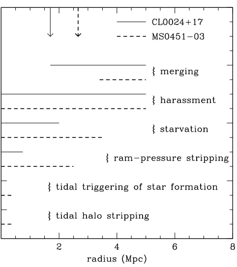
In the schematic diagram shown in Figure 1.2, we apply simple scaling relations to estimate the regimes of inﬂuence for several key physical processes which could be

acting on infalling galaxies. Following the procedure described in T03 for Cl 0024, we construct a simple mass model for each cluster, assumingρ∝r−2 with total mass derived from X-ray measurements (Table 1.1), and allow a galaxy to freely fall from the outskirts on a radial orbit. Under this model, we estimate the radius at which

(27)

Figure 1.2 Schematic diagram indicating the cluster-centric radius over which each of several listed physical mechanisms may be effective at fully halting star formation or transforming the visual morphology of a radially infalling galaxy. Each physical mech-anism listed can act effectively over the radial range indicated by the solid (Cl 0024) or dashed line (MS 0451). Each regime of influence was calculated according to the simple models described in T03 for Cl 0024, using the global cluster properties given in Table 1.1. The virial radius of each cluster is marked with an arrow at the top.

galaxy mergers are possible (see T03). Variation in the physical conditions and orbital characteristics of galaxies will, of course, matter a great deal, but this simplistic case

yields conservative estimates of the maximal radial range over which each process could operate within each cluster.

From Figure 1.2, we see that ICM-related processes, such as gas starvation (Larson et al. 1980; Bekki et al. 2002) and ram-pressure stripping (Gunn & Gott 1972) begin

to aﬀect galaxies at much larger radius in MS 0451. An important caveat, however, is that the role of diﬃcult-to-observe shocks in the ICM are unknown, and are not

accounted for in Figure 1.2 (but see Chapters 3 and 6). Similarly, the two clusters’ diﬀering masses set the radial regions where galaxy merging will be eﬀective; because

(28)

fast for mergers to occur at a higher radius than in Cl 0024.

The diﬀering regimes of inﬂuence for the physical mechanisms illustrated in Fig-ure 1.2 provide the key template for our attempt to disentangle the relative importance

of the various processes. By surveying the galaxies of both clusters for signs of recent transformation or disturbance, across the entire radial range to ∼5 Mpc, we hope to associate the sites and characteristics of galaxies in transition with the likely causes from Figure 1.2.

An important limitation of Figure 1.2, however, is that it does not take into account the variations in overall assembly state and level of substructure between each

cluster. The eﬀects of tidal processes and galaxy–galaxy harassment, for example, should occur in much the same regions across both clusters, according to Figure 1.2,

yet in reality they may very well diﬀer greatly between clusters depending on how well each is virialized. Therefore, Figure 1.2 can only be used as a guide, and we must

carefully consider throughout this thesis the eﬀects that large-scale cluster assembly and irregularities may have on galaxies as well.

1.3

Plan of the Thesis

In this section, we outline our plan for leveraging our wide-ﬁeld surveys of Cl 0024 and MS 0451 into a better understanding of the physics behind galaxy transformations

in clusters. Before delving into analysis of the various galaxy populations in each cluster, we ﬁrst introduce, in Chapter 2, the characteristics of the data set and sample

selection, as well as key reduction and analysis techniques that are common to the investigations presented in later chapters. We discuss the optical HST mosaics along with the complementary ground- and space-based imaging from the X-ray to mid-IR. We also describe our extensive ground-based optical spectroscopy, primarily obtained

(29)

(30)

redshift. As our ﬁeld sample is assembled from foreground or background galaxies

identiﬁed in the course of our observations of Cl 0024 and MS 0451, they have been observed in an identical fashion, thus minimizing any biases. By comparing cluster

galaxies to their counterparts in the ﬁeld, we can pinpoint the locations and strengths of cluster-related processes by identifying peculiarities in star formation or galaxy

dynamics that occur only in the cluster population and not in the ﬁeld. Then, armed with a better understanding of the physics that drives galaxy transformations at

this particular redshift, we can make informed predictions for the processes aﬀecting galaxies at other redshifts, even though the precise conditions within clusters vary

and evolve with time.

1.3.2

Using E+S0s as Sensitive Indicators of Interaction

In Chapter 3, we consider spectral diagnostics of galaxy evolution restricted to E+S0

members of Cl 0024. In the local universe, cluster early-type galaxies are an ex-tremely homogeneous population in terms of their stellar populations and structural

properties (e.g., Dressler et al. 1987; Djorgovski & Davis 1987; Bower et al. 1992; Bender, Burstein, & Faber 1992). By studying these galaxies at intermediate redshift

and contrasting their spectral properties with those of their counterparts in the ﬁeld and local universe, we are sensitive to even very subtle signatures of recent and

cur-rent environmental interactions. In this sense, we explore early-type galaxies as “test particles” of recent activity. This study has yielded two key results:

By constructing the Fundamental Plane (FP) of Cl 0024, we observe that elliptical and S0 galaxies exhibit a high scatter in their FP residuals, equivalent to a spread

of 40% in mass to light ratio (M/LV). The high scatter occurs only among galaxies in the cluster core, suggesting a turbulent assembly history for cluster early types,

perhaps related to the recent cluster–subcluster merger (Czoske et al. 2002).

Around the virial radius of Cl 0024, we observe a number of compact,

(31)

raise the possibility that the observed activity is caused by a rapidly acting physical

process: two candidates are galaxy harassment and shocks in the ICM, though we return to these objects in Chapter 6 to consider the possibility that mergers are

responsible.

1.3.3

Kinematic Disturbances in Spiral Disks

While E+S0 galaxies do prove to be sensitive indicators of environmental interaction,

it is the spiral galaxies that of course host the bulk of star formation within and around these clusters. In Chapter 4, we probe for kinematic disturbances in spiral disks by

measuring resolved rotation curves from optical emission lines, and constructing the Tully-Fisher relation (Tully & Fisher 1977) for spirals across Cl 0024 and MS 0451.

We find that the cluster Tully-Fisher relation exhibits significantly higher scatter than the field relation, in both V and KS bands. In probing for the origin of this dif-ference, we find that the central mass densities of star-forming spirals exhibit a sharp break near the cluster virial radius, with spirals in the cluster outskirts exhibiting

signiﬁcantly lower densities. We argue that the lower-density spirals in the cluster outskirts, combined with the high scatter in both KS- and V-band TF relations, demonstrate that cluster spirals are kinematically disturbed by their environment, even as far from the cluster center as twice the virial radius. We propose that such

disturbances may be due to a combination of galaxy merging and harassment.

1.3.4

When Stellar Population and Morphology Tell

Con-ﬂicting Stories

Analysis of just the early types or just the spiral populations of these two clusters provide valuable clues to the environmental processes that may be acting. However,

the most powerful method of tracking galaxy evolution across Cl 0024 and MS 0451 involves the identiﬁcation and study of “transition galaxies”—galaxies whose stellar

(32)

(33)

a slower pace, with galaxy–galaxy interactions continuing to play a role along with

“starvation” by the ICM.

Using our successful model for the sites and strengths of the various important

physical processes, in Chapter 7 we asses future opportunities for testing our conclu-sions in several diﬀerent manners at a variety of redshifts. We also discuss how our

simple picture of evolution in clusters ﬁts in with the popular picture that is emerging on the role of AGN- or star-formation fueled feedback as a mechanism for halting star

(34)

Chapter 2

A Wide-Field Survey of Two Intermediate

Redshift Galaxy Clusters: Characteristics

of the Survey

We describe our comprehensive wide-ﬁeld survey of two intermediate redshift galaxy clusters, Cl 0024+17 (z = 0.395) and MS 0451–03 (z = 0.540), which forms the basis of the investigations presented in later chapters. For both clusters, optical HST

mosaics are complemented by ground- and space-based imaging from the X-ray to mid-IR, as well as extensive ground-based optical spectroscopy, primarily obtained

with DEIMOS on Keck II. Observations in all bands cover an area extending from the cluster core to the turn-around radius in the cluster outskirts, >5 Mpc physical radius. Together, Cl 0024 and MS 0451 have been observed in more depth and in more wavelength ranges than perhaps any other systems at intermediate redshift. We

describe here the characteristics of the data set and sample selection, as well as key reduction and analysis techniques that are common to the investigations presented

in later chapters. We also present our full spectroscopic catalogs, which we make available to the community.

2.1

Imaging

The keyHSTimaging of Cl 0024 and MS 0451 have been introduced and described in T03 and G. P. Smith et al. (2007, in preparation), respectively. Details of the image

(35)

(36)

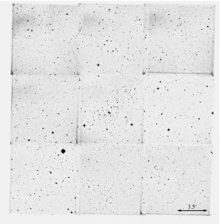
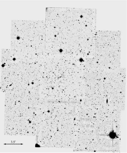
Figure 2.1 Mosaic of 39 WFPC2 images of Cl 0024, arranged as they are distributed on the sky. The locations of all spectroscopically conﬁrmed cluster members are marked as blue circles. The large black circle indicates the virial radius of the cluster, 1.7 Mpc, corresponding to 5.4 on the sky. Cluster members located outside of the

(37)

(38)

for Cl 0024 and MS 0451 are displayed in Figures 2.3 and 2.4, respectively.

The HST and near-infrared data are supplemented with wide-ﬁeld ground-based optical imaging. We make use of BVRI-band imaging of Cl 0024 with the 3.6 m Canada-France-Hawaii Telescope (CFHT) using the CFH12k camera (Cuillandre et al. 2000), full details of which are available in Czoske et al. (2002) and T03. MS 0451

was observed by Kodama et al. (2005) for the PISCES survey through theBVRI-band ﬁlters using Suprime-Cam on the Subaru 8 m Telescope. Full details of these data are

published by Kodama et al. (2005). The CFH12k data reach 3σ depths of B = 27.8,

V = 26.9, R = 26.6 and I = 25.9 in∼0.9 seeing, and the Suprime-Cam data reach 3 σ depths of B = 28.1, V = 27.0, R = 27.3, I = 25.8 in seeing ranging from 0.6 to 1. All near-IR, UV, and HST imaging has astrometry matched to these ground-based optical image sets. The ﬁelds of view of all imaging sets are well matched to the ground-based data.

X-ray observations of Cl 0024 withXMM/Newton(Zhang et al. 2005) andChandra

(Ota et al. 2004), and MS 0451 withChandra (Donahue et al. 2003) reveal markedly diﬀerent X-ray luminosities and temperatures for these two clusters, as discussed in Chapter 1. The clusters’ X-ray properties shed light on the physical processes that

may be working to transform galaxies, and will be discussed further in Chapter 6. However, we do not directly make use of the X-ray images themselves in this work.

2.1.1

Source Extraction and Photometry

Photometry was measured using SExtractor version 2.2.2 (Bertin & Arnouts 1996). For ground-based imaging, we use SExtractor in two-image mode with source

detec-tion performed on the ground-based I-band images. Source detection on the HST

images was performed independently, and then matched to the ground-based

cata-log. For all imaging, we adopt magnitudes from the MAG AUTO measurement of SExtractor.

(39)

3.5’

(40)

3.5’

(41)

to be comparable to the measured NUV FWHM (5.5). We apply an aperture cor-rection to bring the ﬂuxes into agreement with SExtractor-derived total magnitudes (MAG AUTO), and for comparison toMAG AUTOmagnitudes in F814W (Bertin & Arnouts

1996).

For most of our analysis, we convert observed magnitudes into rest-frame absolute

magnitudes usingk-corrections. We use thekcorrectsoftware v.4 1 2 (Blanton et al. 2003) to estimate the necessary k-corrections; we make use of imaging in all available bands from NUV to Ks, modeling each galaxy’s spectral energy distribution and deriving the best-ﬁt correction on a galaxy by galaxy basis. However, we ﬁnd that the

derived k-correction is mostly insensitive to the omission of one or several bands. As the observed and rest-frame bands match well, the requiredk-corrections are typically small, and the rms scatter in k-corrections for all spiral or all early-type galaxies is typically only ∼0.1 magnitudes. We assume a Galactic extinction of E(B–V)=0.056 for Cl 0024 and 0.033 for MS 0451 (Schlegel et al. 1998), and all absolute magnitudes in this work will be expressed on the AB system. Observed optical magnitudes are

quoted on the Vega system, but GALEX photometry is AB.

2.1.2

Morphological Classiﬁcation

For both clusters, reliable morphological classiﬁcation is possible to rest frame

ab-solute V-band magnitude MV = −19.6, corresponding to I = 22.1 in MS 0451 and

I = 21.1 in Cl 0024. Broader classification as early or late type is possible to a fainter limit, MV = −18.0. All galaxies that have spectroscopically confirmed red-shifts and are brighter than this limit are classified visually following the procedure

described in T03 for Cl 0024. In MS 0451, galaxies were classed by R. S. E., and we expect that the typing is accurate to the quoted limits based on previous experience

with ACS imaging of similar depth (e.g., Treu et al. 2005b). Morphologies were as-signed according to the Medium Deep Survey scheme introduced by Abraham et al.

(42)

T=0, 1, 2 are together labeled as “early types” or E+S0s, and all galaxies with T=3,

4, 5 are labeled as spirals. AnM_V∗ galaxy corresponds toI ∼19.5 in Cl 0024 (Smail et al. 1997), whereM_V∗ indicates the absolute magnitude equivalent to the characteristic luminosity,L_∗, of the cluster luminosity function. Our sample with ﬁne morphological distinction reaches to M_V∗ + 1.6, and our deeper sample with only broad classiﬁcation extends toM_V∗ + 3.0.

In Figure 2.5, we display a montage of example MS 0451 cluster members from

our ACS imaging. The chosen galaxies span all morphological types considered in this thesis, at each of three luminosities, roughly corresponding toL_∗ galaxies (MV = −21.2), galaxies near the limit for ﬁne morphological typing (MV = −19.6), and fainter galaxies where only distinction between early and late types is reliable (MV = −18.2). Similar examples of morphological typing are available for Cl 0024 in T03.

Crucial to our strategy of studying galaxy evolution by analyzing early- and

late-type galaxies separately is understanding our accuracy at distinguishing elliptical from S0 galaxies on the one hand, and spirals from S0s on the other. Either type of

misclassiﬁcation could bias our results, especially in comparison to samples at higher or lower redshift, due to the eﬀects of band shifting and surface brightness dimming

on our ability to class galaxies (Smail et al. 1997; Fabricant et al. 2000).

In the following chapters, we take several steps to mitigate any confusion between

classes. These include using the GALFIT software (Peng et al. 2002) to subtract smooth, ﬁtted galaxy proﬁles from each galaxy image. We inspect these residuals for

signs of low-contrast spiral arms, in the case of galaxies classed S0, or else unnoticed disk components in the case of galaxies classed E. More details on these procedures

are detailed in Chapters 3 and 6, but we note that few signs of misclassiﬁed galaxies have been found. We also avoid uncertainties due to misclassiﬁcation by comparing

(43)

5

4

3

2

1

0

T=

-18.2

-19.6

-21.2

Mv

Figure 2.5 Montage of MS 0451 cluster members from ACS imaging. Galaxies span all morphological types from T = 0 (elliptical) to T = 5 (Sc/d), at each of three luminosities, as indicated on the ﬁgure. Luminosities roughly correspond to

(44)

(45)

wavelength was again 6200˚A, providing similar spectral coverage. In 2002, conditions

were fairly poor, with thin clouds frequently interrupting observations. Seeing was approximately 0.7. In 2003, seeing was good (0.5–0.6), though conditions were not photometric. And in 2004, conditions were generally good, with seeing varying between 0.7 and 1.1 across three nights.

We undertook an initial redshift survey of MS 0451 during 2003 October, observing 14 slit masks for one hour each, with the 600 l/mm grating set to central wavelength

7500˚A. This allowed redshift identification for 1300 objects, including 250 cluster members. Targets were selected from the I-band Subaru image discussed above, as the ACS mosaic was not yet available. We first selected objects randomly from the set with I <21.5, and then filled in slit mask gaps with fainter objects (I <23.0).

In 2004, most targeted objects in MS 0451 were selected for deeper follow-up after already being identiﬁed as cluster members in our previous year’s redshift survey.

However we excluded bright cluster members that had already yielded spectra of suﬃcient signal to noise in the 1hr integrations of 2003. We observed 3 masks for 4 hr

each, with gaps between high-priority targets ﬁlled as before with random objects to

I < 23.0. Observations used a 600 l mm−1 grating set to a central wavelength of 6800˚A.

In 2005 October, objects in both clusters were observed with the same spectral

setup and integration times as in 2004, with six masks observed per cluster. However, in 2005 our goal was to follow up on sources detected in both GALEX imaging and

SpitzerMIPS imaging (Geach et al. 2006), and so we ﬁlled masks with these sources preferentially. Targets in these latest observations were not constrained to the same

magnitude limits as previous observations, so some fainter objects were observed, to

(46)

Figure 2.6 A typical spectrum for a galaxy with luminosity near the median of our sample. The entire 1D spectrum is plotted at top, with a segment of the 2D spec-trum displayed below it. We have measured equivalent widths for the spectral lines indicated (see Chapter 3). Overplotted in red is the best-ﬁt template spectrum used in measuring the stellar velocity dispersion, discussed further in Chapter 3.

2.2.1

Data Reduction and Redshift Determination

Spectra were reduced using the DEEP2 DEIMOS data pipeline1 (Davis et al. 2003).

The pipeline performs bias removal, ﬂat ﬁelding, and cosmic-ray rejection. It then separates slitlets and performs wavelength calibration and sky subtraction. For

wave-length calibration, the pipeline uses an optical model of the DEIMOS mask to generate an initial wavelength solution. Arc-lamp frames, consisting of 1 s exposures with Ne,

Ar, Kr, and Xe lamps, are then used to reﬁne the calibration.

From the reduced two-dimensional (2D) spectra, the pipeline extracts

one-dimen-sional (1D) spectra using either a variance-weighted boxcar function, or a variant of the optimal extraction method described by Horne (1986). We perform our analysis

(47)

Ca H 3968 Ca K 3934 [OII] 3727

(48)

(49)

(50)

Table 2.1. Cl 0024+17 redshift catalog

α δ zbest Qualitya Sourceb z δz Nz

(o) (o)

6.845741 17.133789 0.3940 0 2 0.3940 0.0000 1 6.837580 16.997200 0.3966 1 1 0.3964 0.0004 2 6.827622 17.378466 0.3792 0 2 0.3792 0.0000 1 6.821529 17.200779 0.3758 0 2 0.3758 0.0000 1 6.812725 17.213043 0.3813 0 2 0.3813 0.0000 1 6.801040 17.199699 0.3955 1 5 0.3955 0.0001 2 6.765210 17.191099 0.3955 1 5 0.3956 0.0002 3 6.759056 17.073933 0.3790 0 2 0.3790 0.0000 1 6.744001 17.070641 0.3940 0 2 0.3940 0.0000 1 6.737525 17.066620 0.1870 2 3 0.1870 0.0000 1

...

a_{Quality codes: 0 = Quality unspeciﬁed by source, 1 = Secure, 2 =} Probable, 3 = Uncertain

b_{Source codes: 1 = Czoske et al. (2001), 2 = Frazier Owen (private} com-munication), 3 = Hale/COSMIC, 4 = Keck/LRIS, 5 = Keck/DEIMOS

(51)

(52)

pleteness for MS 0451, as a function of absolute magnitude at the cluster redshift,

MV. The corresponding observed F814W magnitudes are given in the axis at the top and bottom of the plot. Overall completeness in both clusters is ∼25% to a limiting magnitude MV = −19.6, roughly 1.5 magnitudes below M∗, and the approximate

point where completeness begins to fall rapidly. Brighter than this limit, our samples

are representative of the clusters as a whole: if we divide the completeness histogram into early- and late-type galaxies, the two subsamples do not diﬀer substantially.

However, in the range−19.6< MV <−18.0, we are biased toward detection of emis-sion line cluster galaxies over absorption line galaxies, and completeness is lower in

MS 0451 than Cl 0024. In the following chapters, we will focus our analysis on cluster members with MV <−19.6, except where speciﬁed otherwise.

Within the HST coverage of Cl 0024, completeness is much higher to this same

MV = −19.6 limit, ∼75%. Likewise, if we confine ourselves to within 3 Mpc radius of each cluster center, completeness also jumps, to 40% and 60% for MS 0451 and Cl 0024, respectively. Both of these figures indicate that we have identified a

sub-stantial fraction of the total population of bright cluster galaxies within the virialized regions of these clusters. Hence, our analysis in later chapters should yield a reliable

and representative picture of the spectral properties and dynamical states of cluster galaxies.

In this thesis, our goals are to combine our HST imaging, used for morphological classiﬁcation and photometry, with high signal/noise Keck spectroscopy to probe star-formation rates, star-star-formation histories, and galaxy kinematics through the various

(53)

Figure 2.9 Redshift completeness of the Cl 0024 and MS 0451 spectroscopic samples, as a function of absolute magnitude MV (middle axis), with the corresponding ob-served F814W for each cluster indicated on the top and bottom axes. Completeness is deﬁned as the number of objects with a spectroscopically conﬁrmed redshift in a magnitude bin (Nz), divided by the total number of objects at that magnitude (N). In the top panel, the dashed line indicates the completeness for just those areas cov-ered by the sparsely sampled HST mosaic of Cl 0024, while the solid line indicates completeness for the full area covered by the ground-based imaging. In MS 0451, the

(54)

Chapter 3

Signatures of Environmental Interaction

in Cl 0024 Early-Type Galaxies

1

In this work, we analyze the properties of early-type (E+S0) members of Cl 0024 as a function of environment, using them as sensitive tracers of the various physical

pro-cesses that may be responsible for galaxy evolution. By constructing the Fundamental Plane of Cl 0024, we infer an evolution in the mean mass to light ratio of early types

with respect to z = 0 of Δ<log(M/LV)>=−0.14±0.02. In the cluster center, we detect a signiﬁcantly increased scatter in the relationship compared to that seen in

local clusters. Moreover, we observe a clear radial trend in the mass to light ratios of individual early types, with the oldest galaxies located in the cluster core. Galaxies

are apparently younger at larger radius, with E+S0s in the periphery having M/LV ratios that nearly match values seen in the ﬁeld at a similar redshift. The strong

radial trend is seen even when the sample is restricted to a narrow range in galaxy mass. Independent spectral indicators used in combination reveal an abrupt

inter-action with the cluster environment which occurs near the virial radius of Cl 0024, revealed by small bursts of star formation in a population of dim early types, as well

as by enhanced Balmer absorption for a set of larger E+S0s closer to the cluster core. We construct a simple infall model used to compare the timescales and strengths

of the observed interactions in this cluster. We examine the possibility that bursts of star formation are triggered when galaxies suﬀer shocks as they encounter the

intracluster medium, or by the onset of galaxy harassment.

(55)

(56)

(57)

af-A key issue is the relationship between trends found in Cl 0024 at various radii

and those found in the ﬁeld at approximately the same cosmic epoch. To facilitate such a comparison we make use of the recent comprehensive study of 163 ﬁeld E+S0s

undertaken by Treu et al. (2005a,b) in the northern GOODS ﬁeld.

A plan of the chapter follows. We brieﬂy recap the key observational data for

this work in §3.2. In §3.3 we discuss our measurements of the stellar velocity dis-persions, the ﬁts to the surface photometry, the various spectral line indices, as well

as an improved estimate of the local environmental densities. In§3.4 we present our results focusing ﬁrst on the Fundamental Plane and the implications of the scatter

and various trends seen as a function of luminosity and location, and correlations between the Balmer absorption and metal line strengths with the velocity dispersion.

We also analyze both radial trends and those seen in the residuals from our global cluster and ﬁeld relations. In§3.5, we develop an integrated picture which combines these independent methods and discuss this in light the results of other studies. For consistency with T03, in this chapter we have adopted the cosmology used in T03

(H₀ = 65.0 km s−1, Ωm = 0.3, ΩΛ = 0.7).

3.2

Observations

We base our current investigation on the comprehensive spectroscopic and imaging

survey of Cl 0024 described in Chapter 2. In this work, we analyze data for 104 E+S0 galaxies identiﬁed as members of Cl 0024, of which 71 have particularly

high-quality spectra (generally deﬁned in this work to be those for which reliable stellar velocity dispersions were measured). Twelve of these E+S0s (6 high quality) come

from the LRIS observations discussed in Chapter 2 and T03, with the remainder from DEIMOS. Broken down by speciﬁc morphological type, our sample includes 34

galaxies classiﬁed as E, 50 as S0, and 20 as E/S0. Of the galaxies with high-quality spectra available, 27 are E, 38 S0, and 10 E/S0.

(58)

of E+S0 galaxies, and to allow us to analyze the surface photometry of the selected

galaxies. To summarize, the HST survey consists of a sparsely-sampled mosaic of 39 WFPC2 images taken in the F814W filter (∼I band), providing good coverage of the cluster field out to radius of >5 Mpc (∼14). T03 reported morphological classifications down to I = 22.5. Classifications to a limiting magnitude of I = 21.1 (MV =−19.5) were found to be very reliable, in that several authors, working inde-pendently, agreed upon the morphology for most objects. This included

diﬀerentia-tion between the subtypes E, E/S0, and S0. While ellipticals and S0s were grouped together in T03, it is useful in this work to detect any diﬀerences between the

pop-ulations of Es and S0s: if spirals are actively transforming into S0s at z ∼ 0.4, we might expect to detect diﬀerences in the stellar populations of the two groups.

Although face-on S0s are notoriously hard to distinguish from ellipticals, espe-cially at high redshift where S0 disks may be too dim to detect (Smail et al. 1997;

Fabricant et al. 2000), we can partially avoid this diﬃculty by focusing on the bright-est early-type galaxies where all but the faintbright-est disks should be detectable. In this

chapter, therefore, we will report distinctions between E, E/S0, and S0 galaxies for a brighter subset of this sample, toI = 21.1. We additionally employ a technique to further distinguish between E and S0 by examining the residual signals found after subtraction of an axisymmetric de Vaucouleurs proﬁle (§3.3 and§3.4).

3.3

Analysis

The powerful combination of HST imaging and high-quality DEIMOS spectroscopy enables us to combine measures of the kinematic and photometric structure of

clus-ter early types with detailed spectral information that reveals the underlying stellar population. Locally, early-type galaxies show several tight correlations between

(59)

(60)

environ-ties necessary for our analysis: local density, velocity dispersion, surface photometry,

and spectral line indices.

3.3.1

Local Density Measurements

Local density measurements in T03 relied on a statistical ﬁeld subtraction, following

the methods of previous work (e.g., Whitmore et al. 1993; Dressler et al. 1997). While adequate, we can improve on these measurements by making use of our large

spectro-scopic catalog (§2.2), supplemented by the extensive catalog of photometric redshifts from Smith et al. (2005a). These catalogs allow us to eliminate most foreground

and background galaxies, and calculate local densities based only on the positions of conﬁrmed or possible cluster members. A standard method of measuring local

density, ﬁrst introduced by Dressler (1980), involves calculating the area enclosed by the ten nearest neighbors of a galaxy (to MV ∼ −20, following Dressler et al. (1997)). In order to obtain local density measurements for our entire sample of 104 galaxies (I ≤22.5), we modify the method to include all fainter galaxies to I = 22.5 (MV ∼ −18) in the tally of nearest neighbors. Our method is as follows:

Each object withI <22.5 is given a weight between zero and one, according to the procedure outlined below. Then, for each object, we calculate the total area enclosed by a set of neighboring galaxies whose cumulative weight equals about 10. (Fractional

weights are common, so the total weight rarely equals exactly 10.) The local density is then calculated by dividing the total weight by the area in Mpc2. Compared to the

method used in T03, this should give a value of Σ₁₀ that is a better reﬂection of the true density of galaxies in the cluster, minimizing errors due to chance superpositions

of background galaxies or groups.

As we wish to include only cluster members in the calculations of local density, we

assign weights to galaxies based on how conﬁdent we are that it is a cluster member. If a spectroscopic redshift is available from the combined catalog, then the object’s

(61)

(62)

density of background objects predicted by our method to the ﬁeld number counts

of, e.g., Abraham et al. (1996a) and Postman et al. (1998). We calculate background count densities of log(N)/deg2 = 4.45±0.05 (toI = 22.5) and 3.90±0.07 (toI = 21.1). Our predicted counts agree with both Abraham et al. (1996a) and Postman et al. (1998), within the uncertainties, for both magnitude limits. As an additional check

on the uncertainty in Σ₁₀ measured to our deeper limit (I = 22.5), we calculated a density (Σ₅) for a total weight of 5. The rms variation between Σ₅ and Σ₁₀ is about

25%. Conservatively, we adopt this as the uncertainty in Σ₁₀. Σ₁₀ for each object, along with other basic properties, are listed in Table 3.2.

3.3.2

Stellar Velocity Dispersions

We are able to measure velocity dispersions only for our brighter sample of early-type members (I < 21.1), as our spectra of fainter galaxies do not have suﬃciently high signal to noise. In order to determine velocity dispersions, we ﬁt to a grid of stellar templates degraded to the instrumental resolution and smoothed to various velocity

dispersions (van der Marel 1994). A high-quality spectrum for an object near our magnitude limit is displayed in Chapter 2 as Figure 2.6, with the best-ﬁtting template

spectrum overplotted.

To determine the signal/noise limit at which our velocity dispersion measures

become unreliable, we performed a series of Montecarlo simulations. We construct fake galaxy spectra from stellar templates smoothed to the resolution and pixel scale of

DEIMOS (for the 900 line/mm grating), truncated to an identical length of∼2600˚A, convolved with a Gaussian of various widths to simulate diﬀerent velocity dispersions,

and degraded to a variety of signal to noise ratios. We then attempt to recover the velocity dispersion of the fake galaxy by running the same code as above.

(63)

a somewhat stricter limit (S/N > 8) on the spectra observed with LRIS and the DEIMOS 600 lines/mm grating which have slightly worse spectral resolution. Only 10 high-quality spectra have S/N < 10, so our results are fairly insensitive to these choices. Table 3.3 lists all galaxies with high-quality spectra, along with their velocity dispersions, formal errors, and the mean signal/noise of the spectrum.

The typical uncertainty in our velocity dispersion measurements is ±10%. These errors are dominated by diﬀerences in σ that depend on the template spectrum used, though systematic errors rise to become equally important as we approach the signal to noise limit. Of the early types where we measured velocity dispersions, there were

three galaxies in common with an earlier study of Cl 0024 by van Dokkum & Franx (1996); the velocity dispersions quoted in van Dokkum & Franx (1996) match ours

in all three cases, with < δσ/σ >=−0.02±0.13. Treu et al. (2005b) derived stellar velocity dispersions from DEIMOS spectra using a similar method to our own. They

pursued several tests to determine the accuracy of their dispersions, and found an rms uncertainty of ∼ 12%, in agreement with our own uncertainty estimates. For more discussion of such accuracy tests, see Treu et al. (2005b).

For each galaxy, we apply a correction to match the central velocity dispersion

measured through a 3.4 aperture at the distance of Coma, following the prescrip-tion of Jørgensen, Franx, & Kjærgaard (1995a). This choice of aperture size for the

correction is somewhat arbitrary, but is a common choice for studies of early-type galaxies at low to intermediate redshift (e.g., Kelson et al. 2000b; Wuyts et al. 2004)

because it facilitates comparison to local measurements of the Fundamental Plane (e.g., Jørgensen, Franx, & Kjærgaard 1996). The magnitude of this correction

de-pends on the physical scale over which the 1D spectrum was extracted, which varies from object to object. The average correction applied is 6.6%± 0.4%. Corrected velocity dispersions are denoted by σ₀, and are listed in Table 3.3.

3.3.3

Surface Photometry

(64)

(65)

μV =I814W + 2.5 log (2πR2e) + ΔmV I−AI −10 log (1 +z) =I₈₁₄W + 5 log (Re) + 1.29±0.04

where AI = 1.95E(B−V) (Schlegel et al. 1998) corrects for galactic extinction, the redshift term accounts for cosmological dimming, and ΔmV I is thek-color correction. In the second line of the above equation, we insert our adopted values: ΔmV I = 0.85±0.03, adopted from calculations by Treu et al. (2001a),AI = 0.11±0.01 from Schlegel et al. (1998), and z ∼0.395. Note that this value of ΔmV I is in agreement with our own k-correction estimates from the multi-band photometry described in Chapter 2.

Since we only measure surface photometry for our brighter sample of galaxies

(I <21.1), formal statistical errors in the measured parameters are very small: less than 0.05 in Re, and 0.05 in magnitude. We estimate that systematic errors are double these values, and adopt 0.1 and 0.1 mag as typical errors inReand magnitude, respectively. There may be additional uncertainty inRe and μV related to the choice of a de Vaucouleurs profile over other structural forms, but previous work (Fritz et al. 2005; Kelson et al. 2000a; Saglia et al. 1993) has shown that the combination of Re and μV that enters into the Fundamental Plane (see §3.4) is largely insensitive to the galaxy profile adopted. Figure 3.1 shows three example fits, for galaxies classified as E, E/S0, and S0. For each galaxy, we display the original galaxy image, the best-fit

model image, and the residuals. As might be expected, the residuals are smaller for

the fit to the elliptical galaxy; the residuals for the S0 galaxy clearly show a disk component that is not well fit by a de Vaucouleurs profile.

We observed two clear edge-on S0s which had to be removed from our sample of high-quality spectra, due to the uncertainty in trying to ﬁt a de Vaucouleurs proﬁle

(66)

Residuals Model Image

S0 E/S0

E

Figure 3.1 Example surface photometry fits, for galaxies classified as E, E/S0, and S0. Top row is the galaxy image. Middle row shows the GALFIT model image. Bottom row shows the residuals of the image fit to model.

by more than 0.75—the two magnitudes for most galaxies in our sample match to much better than 0.75 magnitudes. None of these four galaxies are included in the

previously deﬁned sample of 71 high-quality early types, though they are included in the larger sample of 104 galaxies. The photometric parameters for the high-quality

galaxies are listed in Table 3.3.

(67)

adopted errors on our measurements. We exclude one additional galaxy that we have

in common with van Dokkum & Franx (1996), as it exhibits a disturbed morphology (the triple nucleus galaxy discussed in their paper).

3.3.4

Line-Strength Measures

We measure the strengths of several diagnostic spectral lines for the entire sample of early-type galaxies (to I < 22.5). In order to best probe the stellar population of each galaxy, we select a set of indices that are sensitive to a range of star-formation histories and metallicities. Emission lines, such as [Oii], [Oiii], and sometimes Hβ

indicate ongoing star formation (or possibly nuclear activity). Balmer absorption lines, such as Hγ and Hδ are sensitive to recently completed star formation; these lines are strongest in A-stars, which contribute prominently to a galaxy’s integrated starlight within the ﬁrst Gyr after a burst of star formation. We also measure several

metallicity indicators, such as Mg₂, Mgb, Fe5270, Fe5335, and the composite index [MgFe], which is deﬁned as:

[MgFe] ≡

Mgb(0.72∗Fe5270 + 0.28∗Fe5335)

In the local universe, [MgFe] seems to be insensitive to variations inα-element abun-dance (Thomas et al. 2003), making it a valuable tracer of total metallicity.

Where possible, we adopt the Lick index deﬁnitions to measure the strength of each spectral line (Worthey et al. 1994). In the Lick system, the equivalent width of a line

is measured by defining a wavelength range to either side of a main index bandpass. The mean level of each sideband is determined, and a straight line is fit, defining

the “pseudocontinuum” across the index bandpass. The equivalent width of the line within the index bandpass is then measured with respect to the pseudocontinuum

level. The Lick system does not include an index for [Oii], so we adopt the one deﬁned by Fisher et al. (1998). In Figure 2.6 (Chapter 2), we have plotted an example

(68)

For clarity, the results in §3.4 will concentrate primarily on three representative sets of measurements: [Oii], (HγA+HδA), and [MgFe].

Table 3.3 lists the strengths of several key spectral lines for all 104 galaxies in our

sample. These raw indices are suitable for examining environmental trends within our own data set, but in order to make a proper comparison to other published

data or theoretical models, we must carefully correct for any systematic diﬀerences between each set of measurements. In particular, index strengths are known to vary

with the spectral resolution of the data. While we attempt to compare our data only to measurements made at high spectral resolution, to take full advantage of the

high resolution available with DEIMOS, in some cases we are forced to degrade the resolution of our spectra to match that of the comparison data or model.

In §3.4 and §3.5, we will compare some of our results to the stellar population models of Bruzual & Charlot (2003), which include full synthetic spectra at a

res-olution of 3˚A; this is the closest match available to the intrinsic resolution of our DEIMOS spectra (∼1˚A). We will also examine the Balmer–σ relation in comparison to data measured at 10˚A resolution (Kelson et al. 2001), the approximate resolu-tion of the original Lick system (Worthey et al. 1994). Therefore, we convolved our

DEIMOS spectra with Gaussians to produce degraded spectra at both 3˚A and 10˚A resolutions. We then remeasured the relevant spectral line indices. While not included

in Table 3.3, spectral index measurements from our degraded DEIMOS spectra are available from the authors by request.

To compare our Balmer–σ relation to previous work by Kelson et al. (2001) on the redshift evolution of this correlation, we apply an aperture correction to our HδA and HγA line strengths; we adopt their estimate that the quantity (HδA+HγA) varies with aperture as:

Δ (HδA+HγA) = 1.78±0.16Δ log (Dap)

(69)

(70)

M = 5σ2RE/G. To estimate a stellar mass for a galaxy with no available velocity dispersion, we ﬁrst determine the typical M/LB for a local galaxy of this luminos-ity from Gerhard et al. (2001), and correct M/LB to M/LV by subtracting a factor equal to log(M/LV) −log(M/LB) = −0.06, estimated from the typical colors of nearby early-type galaxies. We then correct for redshift evolution in M/LV (based on our Fundamental Plane results below), and multiply by the observed luminosity of the galaxy:

log(M) log(M/LV)+<Δ log(M/LV)>+ log(LV)

For galaxies with velocity dispersions, masses estimated in this way are consistent with the calculated dynamical masses (Δ log(M/M) =±0.3). We then ﬁt a straight line to measured [Oii] versus speciﬁc star-formation rate (M/Mgal yr−1), to yield a conversion relationship between the two.

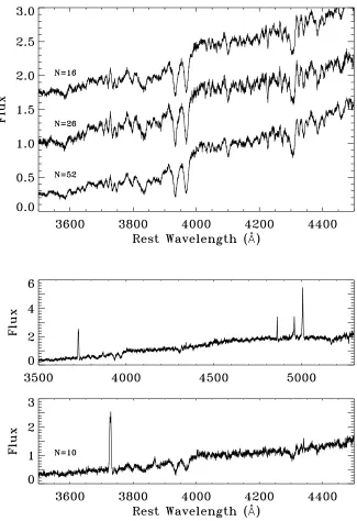
In order to visualize overall trends in the spectral properties of cluster early types, we also produce a series of coadded spectra for each radial zone. Each spectrum is

normalized, shifted to the rest frame, and then coadded. Bad pixels and sky lines are given zero weight in the addition. This method provides a snapshot of what the

aver-age spectrum of each ensemble of galaxies looks like. While weighting by luminosity would better represent the integrated stellar population of each ensemble, in practice,

the coadded spectrum is dominated by the brightest galaxy in each group. We must be careful, however, in interpreting diﬀerences between the coadded normalized

spec-tra for each radial zone: each coadded spectrum will reflect an ensemble of galaxies with a different average size and magnitude. Therefore, it is difficult to separate

ra-dial trends in the spectra from trends with magnitude or size. These coadded spectra will be discussed below in conjunction with the environmental trends in the spectral

(71)

3.4

Results

3.4.1

Cluster: Empirical Scaling Laws

Before we examine environmental trends in galaxy properties, we present the overall

Fundamental Plane, [MgFe]–σ relation and the Balmer–σ relation for the cluster sample with high-quality spectra, and discuss how each has evolved between z ∼0.4 and the present epoch.

3.4.1.1 The Fundamental Plane

Previous studies have traced a mild shift in the intercept of the cluster FP with redshift (Fritz et al. 2005; Wuyts et al. 2004; Kelson et al. 2000b). This seems to be

consistent with passive luminosity evolution of stellar populations with a high redshift of formation (Wuyts et al. 2004), though biases due to morphological evolution are

diﬃcult to quantify. However, most earlier studies have concentrated on measuring the evolution of the FP from data taken in intermediate or high redshift cluster cores.

With our broader spatial coverage, we can uncover any signiﬁcant diﬀerence in the meanM/LV of early types as a function of radius. Our sample also extends to fainter magnitudes than previous studies at z ∼0.4, allowing us to probe M/LV for smaller early types that perhaps formed later than the most massive cluster ellipticals.

Figure 3.2 presents the FP of Cl 0024 compared to that of the Coma cluster, adopt-ing the parameters determined locally by Lucey et al. (1991): α = 1.23, β = 0.328, and γ =−8.71, where the fundamental plane is deﬁned as

log(Re) =αlog(σo) +βμV+γ

(72)

Figure 3.2 FP of Cl 0024, compared to Coma cluster (solid line). Symbols represent diﬀerent morphologies, as indicated. Dotted lines correspond to the expected shift in FP zero point from Coma to z ∼0.4, for SSP models with zf = 2.0,3.0,6.0.

Δ log (M/LV)=Δγ/(2.5β)

(73)

(74)

(75)

(76)

(77)

Figure 3.3 Top: [MgFe]–σat resolution of 3˚A. The solid line is the best least-squares ﬁt to our data, excluding the outlier points atσ ≥300 km s−1. Bottom: (Hγ+Hδ)–σ

at resolution of∼10˚A, compared to Kelson et al. (2001), at same spectral resolution. Indices are corrected to match the aperture used by Kelson et al. The solid line represents the best-fit relation from Kelson et al. (2001). The dashed line is the line of best fit to our data. The scatter is large, so our best-fit relation is highly uncertain. In both panels, velocity dispersi