A Content-Based Routing Protocol for Mobile Ad-Hoc
Networks Using a Distributed Connected k-Hop
Dominating Set as a Backbone
Master Thesis
Wouter Klein Wolterink
Date December 7, 2008 Committee Dr. ir. G.J. Heijenk Dr. ir. M. de Graaf Dr. ir. G. Karagiannis Institution University of Twente
Faculty Electrical Engineering, Mathematics and Computer Science (EEMCS) Group Design and Analysis of Communication Systems (DACS)
Abstract
This report describes the design, implementation and analysis of a content-based routing (CBR) system for a mobile ad-hoc network (MANET) that uses a backbone of flexible size to route its content over. Nodes that are not part of the backbone have a path towards it. By changing the size of the backbone (and thus the length of the paths) an optimum can be found in which routing is at its most effective and efficient. It is shown that for low average node speeds the network is indeed capable of effective and efficient routing, but that at higher speeds the routing paths can no longer be supported.
This backbone used for the CBR system has been created based on a paper by Yang et al. [7]. In their paper they present an algorithm capable of creating and maintaing a connected k-hop dominating set (Ck-HDS). Their algorithm can not be directly applied for a MANET however. This report also describes the design, implementation and analysis of a protocol based on this algorithm.
Contents
Mobile ad-hoc networks and the need for content-based routing Motivation
The design, specification & evaluation of a distributed connected k-hop dominating set algorithm for mobile ad-hoc networks
21
3 Creating and maintaining a connected k-hop dominating set in a mobile ad-hoc network
Designing a protocol able to create and maintain a connected k-hop dominating set in a mobile ad-hoc network
Some notes on backbone networks in mobile ad-hoc networks
25 26 27 27 4 A distributed algorithm for efficient construction and maintenance of
connected k-hop dominating sets in mobile ad-hoc networks
29 4.1
4.2 4.3
The structure of the connected k-hop dominating set A behavioural specification of the algorithm
Examples of operation
29 30 32 5 The design of a protocol for the creation and maintenance of a
connected k-hop dominating set
6 Specification of the protocol 43
6.1
The behaviour of a node at initialization
43 44 45 46
7 Performance evaluation of the protocol 47
7.1 7.2
Performance properties of the implemented algorithm in specific situations
An overall performance analysis of the implemented algorithm
8 Conclusions and future work on the protocol 59
PART III
The design, specification & analysis of a content-based routing system for a mobile ad-hoc network, using the connected k-hop dominating set protocol as a backbone
61
9 An introduction to content-based routing in mobile ad-hoc networks 65 9.1 10 Balancing loads: an introduction to the content-based routing system 71
10.1 10.2
A high level view of the design Design goals
71 72
11 The design of the content-based routing system 75
11.1
The Ck-HDS algorithm as a lower layer The subscription syntax
Creating routing layers with flows Message routing
Creating, maintaining and destroying advertisement and subscription flows with beacons
Beaconing as a means for disseminating advertisements and subscriptions 12 Specification of the content-based routing system 87
12.1 13 Performance evaluation of the content-based routing system 97
13.1 14 Conclusions and future work on the content-based routing system 109
PART IV
Appendices
111 A Results of the content-based routing mobility simulations 113
Glossary 115
Bibliography 117
PART I
Chapter 1
Introduction
1.1 Mobile ad-hoc networks and the need for content-based
routing
A mobile ad-hoc network [2] (or as the acronym goes: MANET) is a type of wireless ad hoc network that consists of a dynamic set of wireless mobile routers (and associated hosts), which we will refer to as nodes. Nodes are interconnected via radio links: if two nodes are within each other’s transmission range they are said to share a symmetric radio link; if one can see the other but not vice versa the first node is said to have an asymmetric radio link to the other node. The dark-coloured elements of Figure 1 show the typical graphic representation of a MANET: a graph in which the vertices represent the nodes and the edges the (assumed symmetric) links. They are free to move at will, creating a continuously changing network topology in which links are created and destroyed in often rapid succession†. MANETs
have no central point of administration, nor are they supported by any fixed infrastructure. Instead, due to the routing capabilities of the nodes themselves, the network is self-organizing. Nodes that are not in each other’s radio range may communicate by means of multi-hop routing, in which nodes that interconnect the communication partners aid in the forwarding of data. Nodes that make up the MANET are often battery-powered with little processing power; links tend to be error-prone with only limited bandwidth.
Figure 1.1. A MANET. The circles around the nodes represent the reach of a nodes’ radio, the arrows represent the direction in which the nodes are moving. The solid lines between the nodes represent communication links; they change as the nodes change their respective locations. Taken together the nodes and links form the vertices and edges of a connected, undirected graph. □
With the steady growth of consumer products that can act as wireless mobile routers (laptops, mobile phones, PDAs), MANETs are becoming increasingly common and resources are shifting towards the edge of the network (i.e., away from wired backbone routers). With this growth, the need for efficient multi-hop routing protocols rises. One can imagine however that efficient end-to-end communication between any two non-neighbouring nodes in a MANET is a task of some complexity [3]. Due to its volatile nature, communicating over a MANET is unreliable and takes a
†
relatively long time, forming a highly unattractive networking environment. Although considerable research efforts have been made and there exist quite a number of proposals for routing solutions, so far no solution has seen widespread (if any) adoption.
Part of the problem of traditional routing in MANETs is that traditional protocols (be them in the application layer, network layer or elsewhere) are address-based, and require that all communication partners know each other. Although this does not seem an unreasonable demand, it does in fact place a burden on routing that can often be avoided. Internet radio stations, peer-to-peer filesharing and group conferences are all examples of applications that are mainly interested in what they exchange; not with whom. Such applications may benefit from content-based routing (CBR).
In CBR there are two actors: someone who has content to offer (usually refered to as a publisher) and someone who wants to receive the content (usually refered to as a subscriber). Both parties do no need to know each other: in stead they rely on the network to route published content to nodes that are interested. The network must therefore base its routing decisions on the information being routed (i.e., the payload of the packets), rather than on the identities of the communicating partners as is the case with address-based routing.
The main problem of any CBR is how to route content both effectively (everyone gets the content they want) and efficiently (content only reaches those parts of a network where it is wanted). Systems are often compared by the percentage of subscribers that get what they want (called the completeness ratio), the percentage of messages that are received that are actually wanted (called the precision ratio) and the overhead that the system’s routing scheme places on the network (this includes the forwarding of the content itself).
CBR was conceived as a means of communication better suited to the peer-to-peer model, which is somewhat similar to a MANET. Quite some research has been performed on CBR, albeit that most of this research has so far focused on static networks. But with the increasing number of MANETs and the promise the CBR model holds, the subject seems likely to draw some more attention in the researching community in upcoming years.
1.2 Motivation
This masters assignment began with the motivation to “design a novel CBR system for MANETs using Bloom filters”. The object was to apply Bloom filters in a similar way as has been done in for instance [4]. This turned out not to be possible however, so the motivation was reduced to (the somewhat vague notion to) “design a novel CBR system for MANETs”. To be further specified based on the results of a preliminary study on the available work on CBR in MANETs, see [5]. A summary of the results of this study has been included in Chapter 9 of this report.
Inspired by an article by Liu, Huang & Zhang [6], which advocates a design in which two communication parties balance the effort they both make to communicate with each other based on their respective needs, I set out to design a system that would be able to adapt to differing needs and circumstances. How this eventually has been done is described in the next section.
The system presented in this thesis makes use of a backbone, of flexible size, that acts as a medium to publishers and subscribers to route their content over. In this the design closely follows the classical publish/subscribe paradigm, in which publishers and subscribers do not communicate directly with each other, but via a medium that bears all communication responsibilities: here the backbone acts as that medium. Each node outside the backbone has a variable-length path of next hops to the backbone. By parameterizing the maximum length of a node’s path to the backbone the backbone’s size is controlled.
The routing overhead of this design is twofold:
1. the overhead to maintain the backbone and a path towards it for each actor outside the backbone;
2. the overhead of routing the actual content.
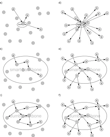
Maintaining the backbone normally gives more overhead than maintaining the paths towards it. Any content published outside the backbone is first routed to the backbone. Inside the backbone routing differs: it is (i) either flooded round the entire backbone or (ii) routed only to those parts of the network that the content is wanted. The first type of backbone is called a dumb backbone, the second type a smart backbone. A dumb backbone has less maintenance overhead but less accurate routing, a smart backbone gives more efficient routing but is harder to maintain (especially as networks become more mobile). The type of the backbone is also parameterized. Finally content is routed to any subscribers outside the backbone. Nodes that are not part of the backbone and are not part of a subscriber’s path towards the backbone do not receive any published content at all.
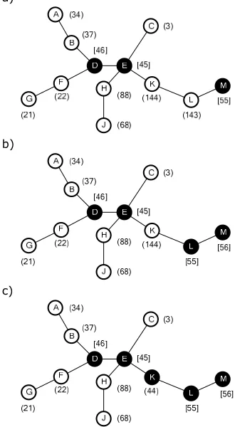
Figure 1.2 shows four instances of the same network: two with a small backbone and two with a large backbone. For each type of backbone-size the number of active participants is also varied: one case has only a few participants, in the other all nodes in the network are participating. Defining content load as the rate with which content is published multiplied by the number of participants in the system, the key point of the design is as follows:
For a given network and a given content load, there exists a backbone size and a backbone type for which the total overhead is minimal.
(1.1)
a) d)
b) e)
c) f)
Figure 1.2 visualizes this statement: in 1.2.a overhead is low because only a small part of the network is involved in maintaining the backbone and its paths, and messages are forwarded relatively efficient. In 1.2.b and 1.2.c however the backbone is much larger, causing increased overhead for maintaining it, while the content load has not changed. If the backbone is dumb (fig. 1.2.c), content will be routed to a large part of the network, causing unnecessary overhead. If the backbone is smart (fig. 1.2.b) it will be routed only to those parts where it is needed. Whether this will make up for the increased effort needed to maintain such a large backbone is unclear however, and depends on the rate with which content is published (for a static number of actors). Comparing Figure 1.2.d, 1.2.e, and 1.2.f, in which all nodes are active participants, it is expected that a large backbone (fig. 1.2.e and 1.2.f) is the most efficient, as it will enable more efficient routing than is the case with a small backbone (fig. 1.2.d). Whether a dumb or a smart backbone is more efficient depends on the rate with which content is published and on whether or not it is at all possible to maintain a smart backbone as mobility increases.
1.3 Approach
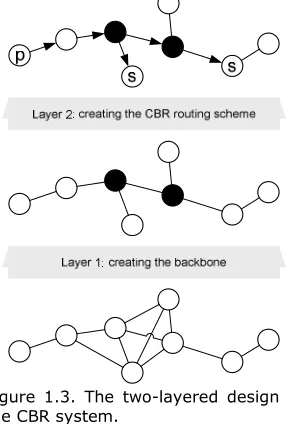
The CBR system has been designed using a two-layered approach: the bottom layer is responsible for creating and maintaining a backbone and giving each node that is not part of the backbone a next hop towards it. The topology that is thus created is used by the upper layer to route content over. Figure 1.3 exemplifies the design.
Figure 1.3. The two-layered design of the CBR system.
assumption that nodes have symmetric radio links. Within the whole system this bottom layer is refered to as the Ck-HDS layer.
In part III the CBR system is presented and analysed. The view that the CBR system has of the network is solely determined by the Ck-HDS layer: a node only communicates with nodes that are presented to it as neighbour. Using this topology the CBR layer tries to build a routing layer to route content over.
1.4
Research goals
The two layers have been designed and analysed separately and their research goals are given in a likewise fashion.
The goal of part II is (i) to design a protocol capable of creating a Ck-HDS in a MANET using only the assumption of symmetric wireless links and (ii) to show by means of simulation how well it is capable of maintaining this set in the face of mobility.
The goal of part III is (i) to design a CBR system that is able to make use of the flexibility of the Ck-HDS algorithm and (ii) to show how well it is able to balance the content load while still maintaining high completeness and precision. Chapter 10 gives a slightly more indept view on the CBR system and formulates a number of specific design questions.
1.5 Outline
This part of the thesis is meant as an introduction for the thesis as a whole. In Chapter 2 the methods that have been used for analysis in both part II and III are discussed.
The second part only concerns the design of a novel algorithm capable of creating Ck-HDS algorithm in a MANET. Ck-HDSs are introduces in Chapter 3, and Yang et al.’s algorithm is explained in Chapter 4. In Chapter 5 the design is presented and discussed; the accompanying specification is given in Chapter 6. Chapter 7 gives a performance analysis of the design by means of simulation and Chapter 8 ends part II with conclusions and some ideas for future work.
Chapter 2
Some notes on analysis
Analysing the performance of a protocol is anything if not hard. It involves choosing a method (construction of a mathematical model, testing or simulation) suited to the protocol and the amount of resources (time, money) at hand. It must have a level of abstraction that covers all (and ideally only) the important details without oversimplifying the design, which could give results that can both be erroneous and ambiguous. The presented results must be statistically valid. Above all it must be repeatable.
Especially in MANETs the number of existing details (multiple layers operating on top of each other, mobility patterns, radio interference) make it hard to perform an analysis that has enough detail to be credible, while still being repeatable. Although live tests will show you whether or not a protocol has any practical value it (i) lacks repeatability, (ii) necessarily encompasses all details making it hard to gauge their effects and (iii) requires a lot of resources. A mathematical model or a simulation, which are both abstractions of reality, will give you full control over all details and perfect repeatability. Mathematically modeling a protocol is often enormously complex however, whereas simulation tools are perfectly suited for just such a case. For these reasons, simulation is the performance analysis method of choice for the MANET community, as well as for this thesis.
Being the analysis method of choice does not guarantee validity. A survey performed by Kurkowski, Camp & Colagrosso [8] on 114 papers published between 2002 and 2005 in ‘Proceedings of the ACM International Symposium on Mobile Ad Hoc Networking and Computing’ showed, amongst others, that 85% of the presented simulations failed to give enough information to ensure repeatability. Other studies [9,10,11] show even more alarming facts. Perhaps the most worrying of these is the analysis performed in [11], where a simple flooding protocol implemented in a number of simulators gave as much results as there were simulators. Simulations, it should be clear, by no means guarantee results that will prove to be perfectly accurate when held against a real world experiment.
In this thesis the advice voiced by Andel & Yasinsac in [9] – who hold that “MANET simulations [should be used] to provide proof of concept and general performance characteristics” – is followed. Both in the case of the Ck-HDS algorithm and the CBR protocol a conceptual model has been implemented that holds all algorithm/protocol functionality described in this document, but few other details. Section 2.2 presents the model in full detail. The model has explicilty been designed to conduct proof-of-concept experiments, not to compare the performance of two protocols in any realistic way.
2.1 Verification
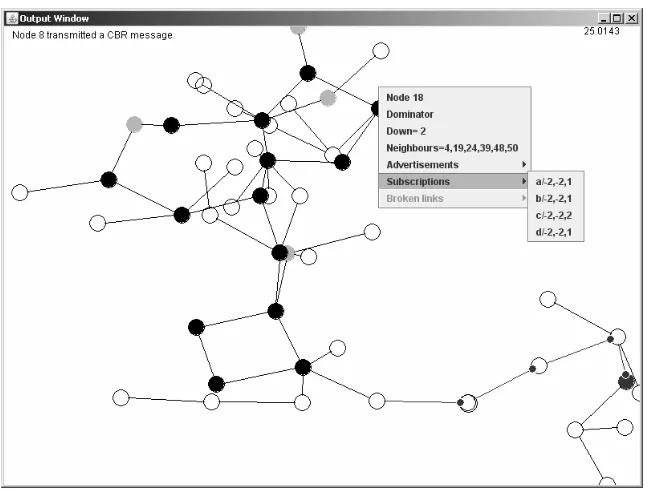
Both the Ck-HDS algorithm and the CBR system have been implemented at a conceptual level (see Section 2.3, A simplified simulation model). In both cases correct operation of the implementation was verified by means of custom made Java-based tool. This tool is able to visualize the behaviour that occurred at a simulation run, by analyzing a log file generated during the run. Figure 2.1 shows a screenshot of the application.
Figure 2.1. The Java-based tool able to visualize both the Ck-HDS system and the CBR system.
2.2 A simplified simulation model
Nodes are in one of three states: inactive, active, or failed. An inactive node is a node that is waiting to become active; a failed node is a node that was previously active but has become inactive. Once a node has entered the failed state it will never leave that state. Only active nodes are able to transmit/receive packets, perform computations and move around.
Nodes are modeled as points in a two-dimensional plain: their position can be represented by an (x,y) coordinate. Mobility is achieved by altering this coordinate. Two nodes can communicate with each other if they are neighbours, i.e., if the distance between their relative positions is smaller than or equal to a node’s
transmission range, which differs per simulation. To give a somewhat realistic feel, both positions and distances presented in this document will usually be expressed in meters.
For mobility the Random Waypoint Model with uniform and stable speeds in [1] was used. In this model nodes move within a defined region. At startup every node chooses uniformly a point within this region as its destination, and draws uniformly a speed from the the range [Vmin,Vmax]. Then whenever a node has reached its
according to the distribution
( )
2=
. This ensures that the average nodespeed for a network is stable at
the simulation and throughout the whole simulation. The only effect that one should still bear in mind is that if nodes are distributed uniformly over a mobility region, they tend to be ‘drawn inside’ at the start of a simulation. This is because of the fact that with the random mobility model nodes on average tend to spend more time in the middle of the mobility region.
System-specific packets are used to exchange information between nodes. Packets can either be addressed to a single neighbour (unicast) or to all neighbours at once (broadcast). Addressing nodes is done by means of unique identifiers, which are pre-assigned to each node and can be compared to a MAC-address. A node is only allowed to perform unicast transmissions with nodes whose identifiers it knows; a broadcast transmission uses no addressing but is delivered to each and every neighbour of the sender.
Nodes are not able to interfere each other’s communication, so both contention and collisions are ignored. In stead a transmission probability is introduced, Tp, which
determines the chance whether a packet reaches a receiver. Communication either succeeds or fails and does so instantaneously (there is no transmission propagation). In case of a unicast transmission the sending node is informed whether a transmission was succesful or not. In case of a broadcast transmission the sending node has no way of telling whether a transmission succeeded or not.
2.3 Creating network graphs for static simulations
To ensure that the networks used in static simulation runs have a random topology but are still connected, the Ad Hoc Network Graph Model was used, described in [12]. Setting R as the transmission range, a graph Gn(a,b,g), consisting of n nodes
and with parameters 0 < a,b,g ≤ 1, is generated with this model from a graph Gn-1
via three steps (a graph G1 is created by simply initializing a node with some given
coordinates):
1. one node u in Gn-1 is randomly chosen by means of the distribution Pr(u) =
g·(1 – g)|N(u)|-1;
PART II
This part focuses on the implementation and evaluation of an algorithm that can create and maintain a Ck-HDS in a MANET. To the best of our knowledge no existing work on the implementation of such an alg exists. The only available work is a small set of theorethical algorithms that all make assumptions that are unrealistic in a MANET, such as perfect topological knowledge. Designing an algorithm from scratch would take too much time, however, so the algorithm that would require the least effort was eventually chosen to be implemented. This was the algorithm presented by Yang et al. in [7], mainly because it was the only available algorithm that addressed maintenance of a Ck-HDS during mobility.
Chapter 3
Creating and maintaining a connected
k-hop dominating set in a mobile ad-hoc
network
Creating and maintaining a connected k-hop dominating set (Ck-HDS) in a static network with stable links is not very difficult. When it comes to a mobile ad-hoc network (MANET) however the volability of the network links becomes a significant problem. After introducing Ck-HDSs in Section 3.1, Section 3.2 shows available work on Ck-HDSs in MANETs. It turned out that, as far as could be verified, there exists no practical solution to this problem. Section 3.3 described how available work of Yang et al. [7] has been used to design such a system.
3.1 Connected
k
-hop dominating sets
Consider a connected and undirected graph G(v,e), such as can be created from a MANET by taking the nodes as vertices and the communication links as edges (see also Figure 1.1). Furthermore assume the following definitions to be true:
Two nodes (or vertices) are said to be connected if they share an
edge. (3.1)
A path is defined as a set of nodes n0···ni-1nini+1···nn wherein for 0 <
i < n each node ni is connected to nodes ni-1 and ni+1, and nodes n0
and nn are respectively connected to nodes n1 and nn-1. The length of
a path is equal to the number of nodes that make up the path: a path n0n1n2 has length 3.
(3.2)
Using the above definitions we make the following incremental statements:
A dominating set (DS) D in G is defined as a set of nodes (or vertices) for which holds that every node in G is either part of D or is connected to a node that is part of D. A node that is in a dominating set is called a dominator. A node that is outside the DS is called a member. If a dominator has any members connected to itself it is also called a dominating node.
(3.3)
A k-hop dominating set (k-HDS) D is a set for which holds that every node in G is either part of the DS or has a path of member nodes of length k or less (excluding the node itself) to a dominator. This path is called a member path.
(3.4)
A connected dominating set (CDS) D is a k-hop dominating set for which holds that for every dominator d in D there exists a path consisting solely of dominators to every other dominator in D.
A connected k-hop dominating set (Ck-HDS) D is a k-hop dominating set for which holds that for every dominator d in D there exists a path consisting solely of dominators to every other dominator in D.
(3.6)
Figure 3.1 shows some examples of (connected) k-hop dominating sets.
a) b)
c) d)
e)
Figure 3.1. Figures a-e show the same graph but with differing dominating sets. The dark colored nodes are dominators. a) shows a 1-HDS, b) shows a C1-HDS, c) shows a C2-HDS, d) shows a Ck-HDS wherein k can have any value higher than 3 and e) shows a C0-HDS. Because the maximum distance to the DS is 0 in e) all nodes are part of the DS.
As the examples in Figure 3.1 show a Ck-HDS is a suitable means for creating a backbone in a network, with the resulting CDS as the backbone itself. By varying the size of k the size of the backbone can be varied: a small k will produce a large backbone with short member paths, while a large k will give a small backbone with long member paths. Such a backbone of flexible size is exactly what is needed in the content-based routing (CBR) system introduced in Part I and fully described in Part III.
3.2 Available work
The idea of creating a C1-HDS (or CDS) in a (mobile) ad-hoc network is far from new, so a number of solutions are available for this simplified version of a Ck-HDS. In general these solutions use either one of the following two strategies:
1. First a DS is created: this is called clustering. Then the dominators making up the DS are connected by means of special connector nodes. Ideally the dominators are connected by means of a minimum spanning tree.
CDS during reconfiguration of the network due to node movement is often considered as a different problem and therefore not always addressed (although in the cases above only [1] does not address maintenance).
When it comes to Ck-HDSs available work is scarce. To the best of our knowledge there exists no actual implementation of a Ck-HDS algorithm specifically designed for MANETs. [7], [25], [26] and [27] each present an algorithm, but all four designs are purely theorethical and are based on assumptions that will often not hold in a MANET, such as perfect topological knowledge. Of these papers only [7] by Yang et al. addresses the issue of maintaining the Ck-HDS during reconfiguration of the network (e.g., due to mobility). Being the most recent paper of the four the paper also shows, for different properties of the algorithm, a number of analyses of its performance compared to the other three algorithms mentioned above. In these Yang et al.’s algorithms it performs either equally good or better than the other algorithms.
3.3 Designing a protocol able to create and maintain a
connected k-hop dominating set in a mobile ad-hoc network
As no protocol exists that is able to create and maintain a Ck-HDS in a MANET (needed for the CBR system described in Part III) it was necessary to design such a protocol myself. This Part describes the design, implementation and analysis of the resulting protocol. The algorithm by Yang et al. has been used as a basis for the design: the design itself mainly focuses on creating a fully distributed version of the original algorithm, capable of operation in a MANET.
Henceforth in this thesis ‘the (orignal) algorithm’ refers to the original algorithm by Yang et al. and ‘the (distributed) protocol’ refers to the fully distributed protocol designed in this thesis.
Yang et al.’s algorithm has been selected as the basis for the new protocol because it was at the time the only available algorithm that addresses the maintenance of a Ck -HDS. It is however far from suitable for use in a MANET. The two main lacunae with regard to its use in a MANET, and which have been the focus of the design efforts of the distributed protocol, are the following:
1. nodes know at all times who their neighbours are; 2. communication has been left unspecified.
In Chapter 4 the algorithm is described in detail. Chapter 5 then describes the design of the protocol based on the algorithm; its is fully specified in Chapter 6. Chapter 7 gives an analysis of the protocol by means of simulation and Chapter 8 gives conclusions and tips for future developments.
3.4 Some notes on backbone networks in mobile ad-hoc
networks
Chapter 4
A distributed algorithm for efficient
construction and maintenance of
connected k-hop dominating sets in
mobile ad-hoc networks
In this chapter the behaviour of Yang et al.’s algorithm and the resulting Ck-HDS structure that it imposes on the network is described. It should be noted that although the algorithm is distributed in its behaviour (nodes independently base their decisions on local knowledge) some parts of it are not distributed. The algorithm is not meant for direct application in a MANET but serves as a starting point for further research such as has been performed in this Part of the thesis.
4.1 The structure of the connected k-hop dominating set
Two nodes in a network are said to be neighbours if they are within each other’s transmission range. Nodes know at all times who their neighbours are. The addition or loss of a neighbour is instantaneously noticed. The set of neighbours of a node x is referred to as the neighbour set of x, or N(x). Each node has an attribute neighbours
that lists all its neighbours. The set of neighbours of x that are dominators is refered to as D(x).
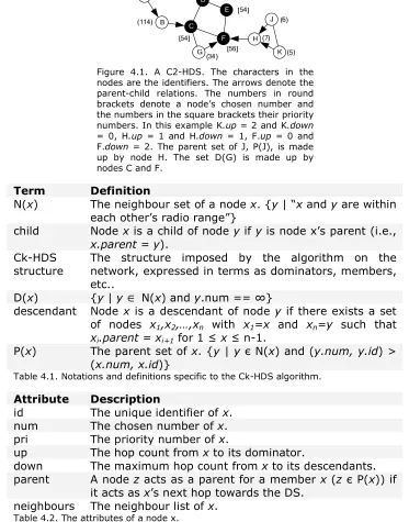
The algorithm structures the network in such a way that a Ck-HDS is created in which the DS may have cycles and each member has a next hop (called the parent) towards the DS, which is the first hop of a path of length k or less. Paths are not necessarily shortest paths. Each node x (either dominator or member) that acts as a parent for another node y (which by definition is a member as dominators have no parents) refers to y as its child. Any children of children (and their children, etc.) are called descendants. So if y should have a node p as its child which in turn has a node
q as its child then both p and q are descendants of x. Node also know their own distance to the DS (in hops), refered to with the attribute up. For a node x the path length of the descendant that has the longest path to x is refered to with the attribute down.
Each node has a chosen number and dominators also have a priority number; these numbers define the Ck-HDS and are constantly revaluated. Member nodes that are situated closer to the DS generally have a higher chosen number; by definition dominators have ∞ as their chosen number. The parent set for a member x (P(x)) is the set of neighbours that all have a higher chosen number than x (dominators don’t have a parent set). The priority numbers are used to impose a hierarchy on the DS when dominators wish to leave the DS.
Figure 4.1. A C2-HDS. The characters in the nodes are the identifiers. The arrows denote the parent-child relations. The numbers in round brackets denote a node’s chosen number and the numbers in the square brackets their priority numbers. In this example K.up = 2 and K.down network, expressed in terms as dominators, members, etc..
Table 4.1. Notations and definitions specific to the Ck-HDS algorithm.
.
down The maximum hop count from x to its descendants. parent A node z acts as a parent for a member x (z є P(x)) if
4.2 A behavioural specification of the algorithm
MANET to demand that every node is present at some artificial point in time, so that construction of the Ck-HDS may commence, this first part of the algorithm is ignored. In stead we focus only on the normal operation.
At the heart of the algorithm lie two conditions which every node must adhere to: 1. For a node x, P(x) must induce a connected subgraph, else x.num = ∞ (x
joins the DS).
2. For a node x there must be a node y in P(x) for which holds x.down + y.up <
k, else x.num = ∞ (x joins the DS).
The first condition ensures that the backbone is at all times connected, proof of this can be found in [7]. The second condition ensures that each member has a path of length k or less to the DS. If any node in a network does not adhere to both these conditions, the Ck-HDS is considered invalid and the node will act so that it adheres to both conditions again. To ensure that the DS does not grow unnecessary large nodes may leave the DS whenever possible; this is explained in Section 4.2.1. The decision for a node x whether P(x) forms a connected subgraph is based on P(x)
itself and the neighbour list of each node y in P(x). Note that the neighbour list does not indicate the role of a neighbour, so node D in Figure 4.1 has no way of knowing that it can simply leave the DS, because nodes C and E are connected by dominator F. In this way cycles will form in the DS whenever there exists a cycle in the network in which nodes are unable to leave the DS and form a connected parent set.
As nodes directly notice the addition or loss of a neighbour they will only act when the structure of the Ck-HDS is invalid. When they do act, they start by exchanging (a subset of) the attributes defined in Table 4.2 with each and every neighbour (the communication details of these exchanges are ignored). Nodes then update their attributes according to the rules that apply to the role the node fulfills, which are explained next.
In the following subsections the exact behaviour of a node is summed up in detail for each possible role that a node can be in: (i) dominator, (ii) member or (iii) a node that has just switched on.
4.2.1 The behaviour of a dominator
A dominator will leave the DS whenever this is possible without breaking the first condition and keeping every node within k hops of the DS. To prevent multiple dominant nodes from leaving the set at the same time – which could cause the DS to be disconnected – the priority property is introduced: only a dominator x that has a higher priority than any other node in D(x) may leave the set. If it leaves the set it sets its chosen number to a value higher than any other node in N(x). If it cannot leave the set it sets its priority lower than any other node in D(x), so that another dominator may try to leave the set. The whole algorithm is as follows:
1. x echanges x.id, x.num, x.parent, x.up, x.down and {y.id | y
∈
N(x)} with every y∈
N(x), and additionally x.pri with every y∈
D(x).2. x updates x.down.
3. If x.pri > y.pri for all y
∈
D(x) then x sets x.num such that x.num > y.numfor all y
∈
N(x). If x.pri ≤ y.pri for any y∈
D(x) then exit.4. If P(x) does not induce a connected subgraph or x.down + z.up ≥ k for all z
∈
P(x) then x resets x.num to ∞, x.pri is set such that x.pri < y.pri for all y∈
D(x) and then the algorithm exits. Otherwise, x sets x.parent randomly to a node y∈
P(x) such that x.down + y.up ≤ k.It should be noted that with this algorithm the priority attribute of a node will always get smaller, never higher. Whenever some node’s priority attribute reaches 0 the value of the priority attributes of all dominators are incremented‡ (with some arbitrary number). This is of course not possible in a distributed network such as a MANET.
4.2.2 The behaviour of a member
A member x must join the dominating set if P(x) does not induce a connected subgraph or if there is no neighbour y
∈
N(x) that can act as a parent such thatx.down + y.up < k. A member node stays faithful to its parent: it will not switch parent until either the parent z moves out of the node’s range or x.down + z.up ≥ k, even when there exist shorter routes to the dominating set (i.e., there exists at least one y
∈
P(x) for which y.up < z.up holds). The whole algorithm is as follows:1. x echanges x.id, x.num, x.parent, x.up and x.down with every y
∈
N(x). 2. x updates x.up and x.down.3. If P(x) does not induce a connected subgraph or x.down + z.up ≥ k for all z
∈
P(x) then x resets x.num to ∞, x.pri is set such that x.pri < y.pri for all y∈
D(x) and the algorithm proceeds to step 5.4. Let z = x.parent. If z
∉
P(x) or x.down + z.up ≥ k then x.parent is randomly* set to a node y∈
P(x) such that x.down + z.up < k and the algorithm exits. 5. x.up is updated.4.2.3 The behaviour of a node that switches on
A node that switches on will preferably become a member, or if that isn’t possible a dominator. The whole algorithm is as follows:
1. x receives y.id, y.num, y.up and N(y) from every neighbour y. 2. x.num is set such that x.num < y.num for all y
∈
N(x).3. If P(x) does not induce a connected subgraph or z.up ≥ k for all z
∈
P(x) thenx.num is set to ∞ and x.pri is set such that x.pri < y.pri for all y
∈
D(x). Otherwise, x.parent is set to a node y∈
P(x) such that y.up < k.4. x.up and x.down are updated.
4.3 Examples of operation
Now that the rules that the nodes follow have been laid out in the previous section, this section exemplifies their behaviour. Figure 4.2 shows a MANET with a valid C2-HDS structure that acts as the starting situation for each example. Figures 4.3, 4.4 and 4.5 respectively show what happens when:
1. a node that switches on can simply join the network as a member, without requiring reconfiguration of the C2-HDS;
2. a node that switches and joins the network requires some reconfiguration of the C2-HDS;
3. a dominator switches off.
‡
Figure 4.2. The reference MANET. The arrows represent the parent-child relations. Dark nodes represent dominators.
4.3.1 A simple join
Figure 4.3. A similar MANET as the one in Figure 4.2. Only the Ck-HDS structure imposed on the network is shown. Node M is added to the C2-HDS structure without reconfiguration of the network.
Figure 4.3 shows how node M joins the network by simply choosing node C as its parent. The only effect this has is that node C will now have its down attribute set to 1 (node E‘s down attribute is unaffected because it already has two paths of length 2). Node M’s chosen number is smaller than any of its neighbours’ chosen numbers, so that P(x) remains connected for any neighbour x in N(M).
4.3.2 A join requiring a reconfiguration of the Ck-HDS
a)
b)
c)
d)
Node M again joins the reference network in Figure 4.4.a, now as a neighbour of node L. Because L.up < 2 does not hold (L.up is 2) node M has no alternative than to join the DS. Since it has no dominator as a neighbour it chooses a random priority number.
Since node L now no longer has a connected subgraph P(L) it also joins the DS, with a priority number lower than that of M. Node K acts likewise and joins the DS with a priority number lower than that of both E and L. When node K has joined the DS it is connected again.
After node L has joined the DS, node M will leave it again (which it can do because it has a higher priority number than node L). Node M assigns itself a random chosen number (since it has no member as a neighbour) and chooses L as its parent.
C2-e)
Figure 4.4. A similar MANET as the one in Figure 4.2. Only the C2-HDS structure of the MANET is shown. Node M’s appearance initiates a reconfiguration of the C2-HDS.
HDS has been fully reconfigured.
4.3.3 Loss of a dominator (recovery of the dominating set)
a)
b)
c)
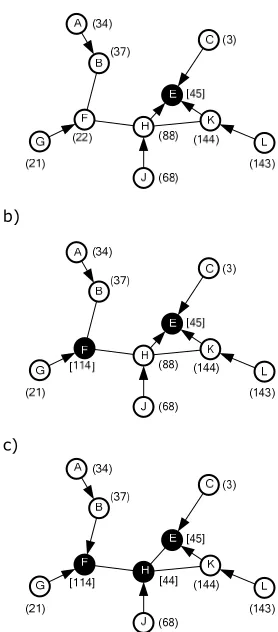
Figure 4.5. A similar MANET as the one in Figure 4.2. The arrows represent the parent-child relations. The loss of dominator D requires a reconfiguration of the C2-HDS.
Figure 4.5.a shows the state of the network right after dominator D has switched off. Node B no longer has a valid parent and node F neither has a valid parent nor a connected subgraph P(F). Either one of the two nodes may act first: in this example we start with node F.
Chapter 5
The design of a protocol for the creation
and maintenance of a connected k-hop
dominating set
This chapter presents a design that aims to lift the functionality of the Yang et al.’s algorithm to a fully distributed protocol. The standard behaviour of the protocol is as has been described in the previous chapter, the protocol only deviates from this behaviour in two places: the choice of a parent (Section 5.4) and the mechanism for leaving the DS. First however the communication details are discussed in Section 5.1 and the way a node constructs and maintains its own view of the network topology in Section 5.2 and 5.3.
5.1 Communication
Yang et al. use a rather abstract mode of communication in their paper, in which nodes are simply able to exchange attributes with their neighbours. They furthermore make use of symmetric radio links, in which nodes can always hear each other. In reality the issue of communication is of course rather more complex than that, and it may have a significant influence on the performance of the algorithm. The mode of communication is discussed below. The assumption of symmetric radio links has been maintained however, because time constraints prevent the redesign of the protocol that would be necessary to incorporate asymmetric links.
Two alternatives exist for communication: unicast and broadcast. Both have some issues when applied as the communication mode of choice. Broadcasting is, in terms of bandwidth efficiency, the most efficient form of communication as it enables a node to communicate its information to all of its neighbours at once, whether it knows those neighbours or not. Broadcasting lacks reliability however: as it does not make use of (negative) acknowledgements, a node has no guarantee that any node will receive its information and will not notice it when a neighbour has moved away. Alternatively, unicast does provide this reliability, making it a more reliable mode of communication ánd a source of accurate network knowledge. However, with only unicast transmissions two nodes that do not know each other never will, so clearly some use of broadcast cannot be avoided.
Because, especially Because it is the most efficient form of communication in a MANET where every node must receive every other node’s information, and it is the only means to discover new communication partners, broadcast was chosen as the method for communication.
5.2 Beaconing
All nodes in [7] have perfect and instantaneous knowledge of their local topology. In this design nodes build and maintain their own view of the network by means of
updated the information contained in it is removed from the node’s view. The use of issues; these are specified in Section 5.6.
Each node regularly broadcasts a beacon containing all its state information. The (mean, as is shown later on) time between two successive beacons of a single node is a system parameter called the beacon interval (BI). The time between between the respective beacons of two neighbouring nodes is calle the inter beacon space (IBS). As nodes receive beacons from other nodes they can construct a view of their local topology. With every received beacon, the view of the network is updated. A beacon that has been received by a node is only valid at that node for a specified amount of time. After a period called the beacon timeout (BT) the beacon is no longer valid; any information contained in it that is not contained in beacons that a node has of other nodes is removed. BT is given as a ratio to BI. If two nodes move away from each other the beacons they have received from each other will eventually time out and the nodes will update their view without the other node in it. Table 5.1 shows the information contained in a beacon. It is almost fully based on the node attributes in the original algorithm. New attributes are introduced in their respective sections. Figure 5.1 shows an example of how nodes keep state of the network. Thanks to the beacons a node knows (with certain probability as new nodes may always come within transmission range and old nodes may always leave) its nodes will often be identified by means of a letter in stead of an integer for readability purposes.
num integer The chosen number.
parent integer The identifier of the node’s parent (-1 if the node is a dominator).
up integer The hop count from the member to its dominator (-1 if the node is a dominator). down integer The maximum hop count from the node to
its descendants (0 if the node has no descendants).
Nx list of identifiers The identifiers of all the node’s neighbours. broken links list of tuples of
identifiers
The broken links that the node knows of. Table 5.1. The attributes that together make up a beacon. The priority attribute used in the original algorithm is no longer used (see Section 5.5).
a) b)
c)
Figure 5.1. Black nodes are dominators, the arrows represent parent-child relations. a) represents a MANET, b) shows the view node A has of the network based on the beacons it received from its neighbours (in this case only node B) and c) shows the view node D has of the network. Node B has a fully accurate view of the network as it receives becaons from all nodes in the network. Table 5.2 shows the beacons of nodes A, B and C. Nodes are identified by means of a letter for readability purposes.
.
The topology of the network continually changes through the (dis)appearance of communication links. There is some delay between the moment a link (dis)appears and the moment that the nodes involved notice its (dis)appearance. Furthermore, the nodes do not notice its (dis)appearance at the same time. Hence, a node may sometimes receive beacons that bear conflicting information. In such cases, newer information is trusted above older information.
Additionally, when nodes are aware that their neighbours have conflicting views of the network that may impair the Ck-HDS, they explicitly incorporate this information in their beacons. Two conflicting views of the network may impair the Ck-HDS when for two previously connected nodes x and y, node x still believes that it is connected to y. The link between two such nodes is referred to as a broken link. If there exists a node z that has both x and y as neighbours, and z is aware of the conflicting views, then z will include the broken link between x and y in its beacon (in its broken links
attribute, see Table 5.1).
cancel their fast respsonse if the first fast response has revalidated the Ck-HDS structre. After node has scheduled a fast response it resumes its previous BI. Table 5.3 lists the critical events and the nodes that are responsible in such a case to
A dominator notices that it has suddenly lost one of its neighbouring dominators, which indicates that the DS may be disconnected. It reacts by sending a fast response that no longer includes the lost node in its neighbour list, thus informing any receiver that the link with its previous neighbour is no longer valid. If the DS is truly disconnected then there must be at least one member x in the network that does not have a connected subgraph P(x), which reacts by joining the DS by means of a fast response.
The two that the child no longer has a valid parent. Of this set of nodes the node with the highest chosen number reacts by also sending a fast response. When the child receives this response it will notice that it has no longer a valid parent, choose a new parent and send a fast response.
A child notices it has lost its parent; it reacts by choosing a new parent and sends a fast response.
The child.
Table 5.3. A number of critical events, the reaction of the Ck-HDS, and the nodes responsible for the reaction.
5.3 Beacon spacing
For the responsiveness of the system it is important that, for sets of neighbouring nodes, the moments that nodes beacon are spaced as evenly over time as possible: ideally each node in a set of X neighbouring nodes has an IBS of BI/X with respect to every other node in the set (see Figure 5.2).
a)
b)
Figure 5.2. The beacon moments of a set of 4 nodes. In a) the beacons are perfectly spaced over time, in b) they aren’t.
neighbouring nodes that have a perfect IBS respond faster to an event to two nodes that haven’t got a perfect IBS.
a) b)
Figure 5.2. Two nodes move apart at time t=1.4. For the case where the inter beacon space is 0.2/0.8, the loss of link AB is noticed at t=2.1 because the beacon node B received at t=1.0 times out. For the case where the IBS is 0.5/0.5 the loss of the link is noticed at t=1.6 because the beacon node A received from B at t=0.5 timed out.
The worst case with regard to the IBS (and thus the average response time of the system) is the case when two nodes beacon close together, called in phase beaconing. Unfortunately this situation is a direct effect of the fast response machenism described in Section 5.2. Indeed, test runs of the implemented algorithm showed how after time large parts of the Ck-HDS were divided into sets of nodes that were beaconing in-phase due to their (often chained) reaction to an event. To counter this behaviour two timing windows are introduced in this section: the beacon window (BW) and the resume window (RW).
The BW is a window of time spaced evenly around a node’s expected beacon moment, in which a node schedules its beacon. Thus, in stead of scheduling a beacon every BI seconds (disregarding fast responses), a node has some random variation in its BI. Introducing such randomness into the system will not prevent worst cases from occurring, and can even bring nodes that previously had their respective beacons perfectly spaced closer together. It does however succesfully ensure that the probability that neighbouring nodes stay in phase with each other for multiple BIs decreases as the size of the BW increases. BW is given as a ratio of BI. Note, however, that the maximum value of the BW should never exceed the BT (the exact timing constraints are listed in Section 5.6). The effect of RW is experimentally tested in Section 7.1.
The RW is the time window in which a node schedules the beacon following a fast response and is given as a ratio to BT. By choosing a suitably large value for RW the chances diminish that neighbouring nodes that responded fast to the same event will beacon in phase (this is experimentally tested in Section 7.3).
5.4 Choosing a parent
Choosing a parent may have impact on the length and connectivity of member paths (the latter being dependent on the former). Solutions for choosing a parent range from the simple (choose a parent at random from the set of nodes in P(x) that have attribute up < k) to the more involved (base the decision on known parent-child relations in the neighbourhood). Furthermore, once a node has chosen a parent it can choose to keep that parent as long as possible (‘stay faithful’), pick a better parent as soon as it finds one or revaluate its parent at a certain time in the future, or at the occurrence of a certain event.
Which strategy for choosing (and keeping) a parent performs best is hard to predict, not only because it differs per situation but also because the performance metric may differ. A strategy that ensures a stable Ck-HDS may provide for very inefficient routing, and vice versa. Which of the two metrics is more important depends both on the environment in which the implemented algorithm will be deployed, and the way it will be used.
Ideally this document would describe a number of strategies for choosing a parent that give the best performance for a given performance metric (e.g. stability, length of member paths) and a given environment (e.g. a static network or a highly mobile one). As this is not possible due to lack of time a single strategy has been chosen, described below. A more in-depth solution such as described above is refered to as future work.
In the implemented algorithm a node x becoming a member chooses a parent at random from the set of nodes Y (yi є Y) for which hold:
1. yi є P(x);
2. yi.up < (k - x.down);
3. there is no yj (yj є Y, yj є P(x), yj.up < (k – x.down)) such that yj.up < yi.up.
A member will furthermore keep its parent until it becomes invalid. This design was chosen with the following (inconclusive, as was argued above) notions in mind:
1. Shorter paths are more stable.
2. Randomness of choice will generally prevent the creation of a single point of failure.
3. Dependency on state information of neighbouring nodes creates vulnerability, as there is a certain probability that the state information is outdated, so dependency should preferrably be kept low.
4. Stability of the Ck-HDS depends on a per-node up to date view of the network. Whenever a member chooses a new parent, the view of its (former) neighbours is outdated: hence, continually choosing a new parent destabilizes the Ck-HDS.
5.5 Dropping the priority number
5.6 Timing constraints
Table 5.4 lists the timing constraints discussed in the previous sections, Figure 5.3 visualizes their boundaries.
Name Unit Range Description
Beacon Interval (BI)
seconds BI > 0 The mean time between any two consecutive beacons of a node. Beacon Timeout
(BT)
ratio to BI BT > 1 The time after which the beacon is outdated.
Beacon Window (BW)
ratio to BI 0 ≤ BW < 2·(BT – 1)
The window in which the beacon will be transmitted; ranges over [BI – BW/2; BI + BW/2].
Fast Response Window (FRW)
ratio to BI 0 < FRW < 1
The window in which a fast response is scheduled; ranges over [0; FRW·BI].
Resume Window (RW)
ratio to BT 0 ≤ RW < 1 The window in which the regular beacon following a fast response is scheduled; ranges over [BT * (1 – RW); BT].
Table 5.4. The parameters that determine the timing constraints of beacons.
.
Chapter 6
Specification of the implemented
algorithm
Below the all the rules governing the behaviour of the protocol are defined. Together with the specification of the beacon and the timing constraints in Chapter 5 this gives a complete definition of the protocol.
6.1 Generic behaviour
Figure 6.1 shows a role-independent, high-level state diagram of a node’s behavioural lifecycle. After a node has switched on it immediately schedules a transmission of a beacon 1 BI later. Any beacons that are received in the interval between the node switching on and the first beacon are used to create a view of the network. When the time has come to transmit, the beacon is constructed based on the node’s view and broadcasted to the node’s neighbours; finally the next regular beacon is scheduled. With its first beacon a node proclaims its role and enters its active state, in which it will beacon regularly, keep its view of the network up to date by means of received or timed-out beacons up to date and (if necessary) respond fast to events that invalidate the Ck-HDS. If an event occurs but a fast response is not necessary then beaconing continues as normal (i.e. with BIs ranging over the interval [BI – BW/2; BI + BW/2]).
Figure 6.1. The generic cycle of behaviour for a node. Function updateView() updates the node’s view of the network based on the newly received information. Function respond() first calls updateView() and if the view shows an invalid CkHDS structure it will respond by sending a new beacon.
Whether or not a fast response is necessary as well as constructing the beacon are role-dependent functions which are explained in the three sub-Sections 6.2, 6.3 and 6.4. First updating a node’s view is explained in the next section.
6.1.1 Updating the view
Whenever a node x receives a beacon from a node y, it will perform the following actions:
1. if y belongs to a new network (explained below) the newNetworkEncountered flag is set;
2. if not already present y is added to x’s view, else the information stored about
y is updated;
3. any link yr (r є N(x)) existing in y’s view is added to x’s view if it isn’t already present;
4. any link yz (z є N(x)) that exists in x’s view but does not exist in y’s view is removed from x’s view and added to the set of broken links;
5. any broken link qz (q, z є N(x)) in y’s view is removed from x’s view if present;
6. if x is a dominator the set of lost dominators is updated; 7. the set of lost children is updated;
8. if x is a member P(x) is recalculated; 9. x.down is updated.
A node x will conclude that a node y that it received a beacon of belongs to a new network when all of the following holds:
1. x has no previous beacon entry of y; 2. x is not listed as a neighbour of y;
3. none of x’s neighbours are listed as neighbours by y or vice versa (N(x) and N(y) are disjunct).
Whenever the beacon that a node x received from a node y times out, the following actions are performed:
1. y is removed from x’s view;
2. if both x and y are (were) dominators then y is added to the set of lost dominators;
3. if y was a child of x then y is added to the set of lost children; 4. x.down is updated;
5. if y was the parent of x then x’s parent is updated.
6.2 The behaviour of a dominator
A dominator x deems a fast response necessary if: 1. the newNetworkEncountered flag is set;
2. the set of children that x has lost is non-empty; 3. all of the following hold:
a. there exist in x’s view two nodes y, z (y, z є N(x)) for which hold that
y.parent == z.id;
b. the link yz does not exist in x’s view;
c. there exists no node q (q є N(x), q є N(y)) for which holds (q.num, q.id) > (x.num, x.id);
The algorithm for creating a beacon as a dominator is as follows: 1. Set x.up = 0 and x.parent = -1
2. Let C be the set of x’s children (i.e., ci.parent == x.id) and cj the child for which
holds that cj.down ≥ ck.down for any k. Then set x.down = cj.down + 1.
3. Try to set x.num such that there is no member y (y є N(x)) for which holds
y.num ≥ x.num. If this is not possible set x.num = ∞ and exit.
4. If P(x) gives a connected graph choose a parent by picking a node z at random from the set of nodes Z for which holds: z є P(x), z.up < k and there exists no node y (y є P(x)) for which holds y.up < z.up. Then set x.parent = z.id and x.up = z.up + 1. If P(x) is not connected or if no such parent can be found than set
x.num = ∞.
6.4 The behaviour of a member
A member x deems a fast response necessary if: 1. the newNetworkEncountered flag is set;
2. the set of children that x has lost is non-empty; 3. all of the following hold:
a. there exist in x’s view two nodes y, z (y, z є N(x)) for which hold that
y.parent == z.id;
b. the link yz does not exist in x’s view;
c. there exists no node q (q є N(x), q є N(y)) for which holds (q.num, q.id) > (x.num, x.id);
4. P(x) is disconnected; 5. x.parent
∉
P(x);6. for x’s parent p the following holds: k – p.up ≥ x.down. The algorithm for creating a beacon as a member is as follows:
1. Let C be the set of x’s children (i.e., ci.parent == x.id) and cj the child for which
holds that cj.down ≤ ck.down for any k. Then set x.down = cj.down + 1.
2. If P(x) gives a connected graph go to step 3, else go to step 5.
3. Let p be the parent of x. If p є P(x) and k - p.up < x.down, then set x.up = p.up
+ 1, x.parent = p.id and exit. If p
∉
P(x) or k – p.up ≥ x.down go to step 4. 4. Choose a parent by picking a node z at random from the set of nodes Z forwhich holds: z є P(x), z.up < k and there exists no node y (y є P(x)) for which holds y.up < z.up. Then set x.parent = z.id, x.up = z.up + 1 and exit. If no such parent can be found go to step 5.
6.5 The behaviour of a node at initialization
The algorithm for creating the first beacon of a node is as follows: 1. Set x.down = 0.
2. Try to set x.num one lower than the current minimum value of the chosen number in the neighbour set. If this is not possible because the current minimum already has the lowest possible value assign a random value to x.num. 3. If P(x) gives a connected graph choose a parent by picking a node z at random
from the set of nodes Z for which holds: z є P(x), z.up < k and there exists no node y (y є P(x)) for which holds y.up < z.up. Then set x.parent = z.id and x.up
= z.up + 1. If P(x) is not connected or if no such parent can be found than set
Chapter 7
Performance evaluation
The goal of this chapter is to show well the protocol performs for differing network conditions such as network mobility and network density. Performance is expressed in (i) the ability of the protocol to maintain a connected DS, (ii) to maintain for each member a valid path to the DS, (iii) the average size of the DS, (iv) the average length of a member path and (v) the average node beacon rate.
Testing has been done by means of simulation, using the simplified simulation model described in Section 2.3: a model that does not incorporate existing network-technologies but in stead gives a conceptual representation of a MANET. The results of these tests should therefore be interpreted as a proof of concept, a means to gauge the feasability of the design. In no way are the results directly comparable to the performance results of existing techniques. Static networks have been generated using the Ad Hoc Network Graph Model, ensuring connected and randomly generated networks; for node mobility the Random Waypoint Model with uniform and stable speeds has been used. Both techniques are also described in Section 2.3.
The simplified simulation model allows for complete control and track-keeping of the state and actions of the individual nodes and the network as a whole. Measurements have been made by checking the state of the Ck-HDS structure at determined intervals. A network has a connected DS whenever every dominator has a path to every other dominator consisting solely of dominators. A member has a valid path to the DS when every assigned next hop of the path (i.e., a member’s parent) is within transmission range. Path validity is averaged over all members. During mobile simulations nodes are often dispersed over several networks of nodes: in that case the connectivity of the DS is averaged over all the networks. To ensure that statistics are not skewed too much, single-node networks are not taken into account, as they already by definition have a connected DS. Figure 7.1 shows a number of networks and their combined connectivity. The average node beacon rate is calculated as the average amount of beacon transmissions per node per BI. If for example 5 nodes beacon 12 times during 2 seconds and BI = 1.0 seconds, the average node beacon rate is
1
.
2
0
.
1
2
5
12
=
⋅
.
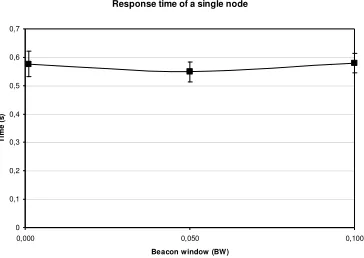
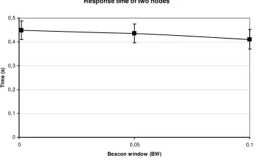
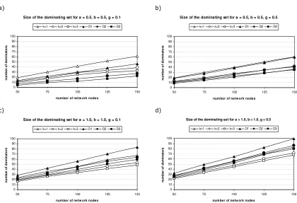
This chapter starts with the analysis of a number of specific performance properties in Section 7.1: the effect of parameters BW and RW is given as well as the response time of a single node and of two nodes on a critical event. Section 7.2 shows the average backbone size and path length for the protocol in a static environment with differing network sizes and densities. These have been measured both for the original algorithm as for the protocol. In the original algorithm a different algorithm is used to construct the Ck-HDS at time t=0, called the Restricted k-Dominant Pruning algorithm. This algorithm has not been described here as it is rather complex and it has not been used in the design of the protocol. It is fully described in [7]. It has been implemented in Java however, and the same static experiments have been performed on it as on the protocol, to compare the initial size of the DS. Finally Section 7.3 gives a full performance analysis on the protocol in a mobile environment with differing average node speeds. The effect of transmission loss is tested by statistically letting 5% of all beacon transmissions fail. Time constraints prevented testing of the protocol in a mobile environment with differing network sizes and densities.
7.1 Performance properties of the implemented algorithm in
specific situations
7.1.1 The effect of the beacon window on the inter beacon space of
nodes that beacon independently
The goal of this experiment is to show whether the IBS of two independently beaconing nodes is influenced by differing values for BW. This has been done by measuring for each beacon the offset of its IBS (with regard to the last beacon of the other node) to the ideal IBS. Before the experiment is described below the details of the ideal IBS and the expected IBS are explained.
Ignoring the randomness introduced by the BW, the expected average time between the consecutive beacons of two independently beaconing nodes (A and B) can be calculated as follows. Suppose that node A beacons every BI seconds as in Figure 7.2. Let X then be the amount of time between the moment B first beacons and A beaconed last. Because A beacons at deterministic intervals X is uniformly distributed over [0,BI> and the expected average E[X] = BI/2. This is equal to the ideal IBS of two nodes (which was previously defined as BI divided by size of the set of neighbouring nodes).
Figure 7.2. The time between the consecutive beacons of two nodes A and B. X is the time between the beacon moment of A and B, moment of A and B, Y is the time between the ideal beacon moment of B and the actual beacon moment of B. Z is the ideal IBS.
For the experiment two nodes are placed outside each others transmission range and are initialized at a randomly chosen moment using a uniform distribution in the time window [0,BI]. For 300 seconds the offset of each IBS to the ideal IBS is measured. The experiment was performed for differing values of BW. Parameters BI, BT, FRW and RW have been kept static at 1.