COMPARISON OF METHODS FOR MODELING UNCERTAINTIES IN A 2D HYPERTHERMIA PROBLEM
D. Voyer, L. Nicolas, and R. Perrussel
Laboratoire Amp`ere (UMR CNRS 5005) Universit´e de Lyon
´
Ecole Centrale de Lyon, 36 avenue Guy de Collongue Ecully 69134, France
F. Musy
Institut Camille Jordan (UMR CNRS 5208) Universit´e de Lyon
´
Ecole Centrale de Lyon, 36 avenue Guy de Collongue, Ecully 69134, France
Abstract—Uncertainties in biological tissue properties are weighed in the case of a hyperthermia problem. Statistical methods, experimental design, kriging technique, stochastic methods, and spectraland collocation approaches are applied to analyze the impact of these uncertainties on the distribution of the electromagnetic power absorbed inside the body of a patient. The sensitivity and uncertainty analyses made with the different methods show that experimentaldesigns are not suitable for this kind of problem and that the spectral stochastic method is the most efficient method only when using an adaptative algorithm.
1. INTRODUCTION
some variability is introduced for the biological tissue properties in a hyperthermia problem. Even if 3D situations are more realistic, a 2D example has been chosen here for focusing the study mainly on the variability aspect. In order to determine the most influential factors and quantify their effects, different approaches are briefly presented and compared in terms of accuracy and computationalcost: a two level experimental design approach [2], kriging approach [3] and finally, stochastic spectral [4] and collocation [5] methods using adaptive sparse grid [6].
2. HYPERTHERMIA PROBLEM
The treatment of a tumor located inside the liver of a patient is considered. The 2D modelhas been obtained from a computed tomography slice of the body.
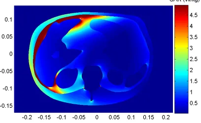
In thefirst step, the electromagnetic properties (permittivityand conductivityσ) of the different healthy tissues are set to the common values used in literature [7] while those of the tumor are based on a specific study of cancerous tissues at radio frequencies [8] (see Table 1). The amplitudes and the phases of four incident waves are adjusted so that to maximize the power absorbed inside the liver and minimize the power absorbed elsewhere in the body (see Fig. 1). More precisely, the quantity we minimize is:
Table 1. Mean values of tissue parameters involved in the hyperthermia problem and range of variation.
Quantity Mean Variation
σ muscle 0.707 ±25%
r muscle 65.972 ±25% σ fluid body 1.504 ±25%
r fluid body 69.085 ±25%
σ bone 0.064 ±25%
r bone 15.283 ±25%
σ marrow 0.022 ±25%
r marrow 6.488 ±25% σ kidney 0.810 ±25%
r kidney 98.094 ±25% σ liver 0.487 ±25%
r liver 69.022 ±25% σ tumor 1.005 ±50%
r tumor 84.342 ±50% σ bowel 1.655 ±25%
r bowel 96.549 ±25%
σ lung 0.558 ±25%
r lung 67.108 ±25%
y=
body=liverσ(τ)|E(τ)| 2
dτ
liverσ(τ)|E(τ)| 2
dτ (1)
whereE is the amplitude of the electric field. As it is not the core of this work, this optimization step will not be detailed.
In the second step, the properties of the different tissues are supposed to be random variables with uniform probability laws while the phases and amplitudes of the four incident waves are maintained at the values found in the first step. For the sake of illustration, the properties of the tissues are assumed to vary in a range of±25% around the mean value except those of the tumor, which vary in a range of ±50%; this distinction is introduced because the properties of tumors are usually less known than those of healthy tissues.
to the tissue properties. For each of the strategies mentioned in the introduction, a specific model for y is assumed and a specific numerical experimental design is built in order to estimate the unknown parameters of the model. Such a design consists in the choice of a set of realizations ornodes for the random variables. Comparisons are proposed in terms of sensitivity and uncertainty analyses.
3. CLASSIC TWO LEVEL EXPERIMENTAL DESIGN
The random input variables are normalized between−1, the low level, and +1, the high level. The model fory is:
y(x) =β0+ 18
i=1
βixi+
18
i=1
j>i
βi,jxixj+. . .+(x) (2)
where x = {xi}i=1,... ,18 ∈ [−1,1]
18 denote the normalized variables. The coefficients {βi}i=1,... ,18 correspond to the main components; {βi,j}i,j=1,... ,18;j>i correspond to the interactions between two
variables; higher order interactions are also considered. The first part of the modelis the regression model and the remaining is the error. This error is supposed to be a random process with azero mean and wheretwo realizations are uncorrelated.
Once a numeric experimentaldesign is built, the estimate βof β
is theordinary least square solution based on the nodes of the design. In statistics, it is also thebest linear unbiased predictor forβ.
In a two level experimental design, the nodes are chosen at the edges of the domain and thus each ˜xi can take the values −1 and +1.
Consequently, the complete design will involve 218 = 262,144 nodes. When the numericalexperiments are expensive in computational resources, the complete design cannot be performed. A solution is to consider fractionalexperimentaldesigns where some effects are confounded. A fractionaldesign is characterized by its resolution: in a resolution III, main components can be confounded with interactions of order 2; in a resolution IV, main components cannot be confounded with interactions of order 2 but two interactions of order 2 can be confounded.
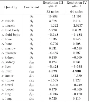
resolution IV. It appears that the properties of the liver and the fluid body have the greatest influence on the value of y; the properties of the muscle have a lower impact. As shown in the next sections, these results are in agreement with those obtained by other methods. On the other hand, the experimental designs give little importance to the properties of the tumor and the bone, which is actually unexpected. Moreover, there is a discrepancy in the estimation of the coefficientsβ6 andβ14between resolution III and IV. In order to refine the results, the resolution should be increased but the numerical cost will also strongly increase: 512 nodes is required for the resolution VI (resolution V does not exist for this example).
Table 2. Results for the fractional experimental design.
Resolution III Resolution IV Quantity Coefficient 218−13 218−12
32 nodes 64 nodes
β0 16.888 17.194
σ muscle β1 3.378 2.514
r muscle β2 −1.222 −2.0237
σ fluid body β3 5.976 6.812
r fluid body β4 −5.348 −5.485
σ bone β5 1.035 0.845
r bone β6 −0.796 0.508
σ marrow β7 0.331 −0.538
r marrow β8 −0.485 0.297
σ kidney β9 0.150 −0.309
r kidney β10 0.124 0.231
σ liver β11 −5.421 −5.935
r liver β12 4.679 4.930
σ tumor β13 −1.812 −1.689
r tumor β14 −1.565 1.322
σ bowel β15 −0.408 −0.249
r bowel β16 0.179 −0.409
σ lung β17 −0.215 −0.120
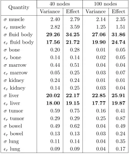
Table 3. Results for the kriging approach: partial variance (%) and totaleffect (%) of the different parameters.
Quantity 40 nodes 100 nodes Variance Effect Variance Effect
σ muscle 2.40 2.79 2.14 2.35
r muscle 2.82 3.59 1.25 1.51 σ fluid body 29.26 34.25 27.06 31.86
r fluid body 17.56 21.72 19.90 24.74
σ bone 0.20 0.28 0.01 0.05
r bone 0.14 0.14 0.02 0.05
σ marrow 0.44 0.51 0.04 0.04
r marrow 0.05 0.25 0.03 0.07 σ kidney 0.24 0.24 0.01 0.01
r kidney 0.14 0.25 0.03 0.04 σ liver 20.02 22.17 22.85 25.91
r liver 18.00 19.15 17.77 19.87 σ tumor 0.59 0.75 0.16 0.41
r tumor 0.29 0.29 0.25 0.87 σ bowel 0.49 0.62 0.04 0.49
r bowel 0.13 0.13 0.03 0.24
σ lung 0.11 0.14 0.04 0.35
r lung 0.09 0.09 0.04 0.17
4. KRIGING
In the kriging approach, the modelof y is composed of a regression model, as in classic experimental design, and of an error whose properties are different from the error given in (2). Indeed, the error is chosen to be a stationary Gaussian process with a zero mean but wheretwo realizations are correlated. From the numeric experimental design, the parameters of the correlation function are estimated and it enables to correct the systematic bias that appears betweeny and the regression modelat the nodes of the design.
nodes, this Latin hypercube is the result of an optimization process of thespace-filling properties.
Two simulations of the hyperthermia problem have been carried out using 40 nodes and 100 nodes. The sensitivity analysis is given in Table 3. For each input random variable xi, the partialvariance and
the totaleffect are computed; those quantities correspond respectively to Var[E[y|xi]]/Var[y], where E[·] denotes the expectancy and Var[·]
the variance, and to the contribution to the variance of xi but also
of the higher order interactions involving xi [11]. It appears that
the properties of the fluid body and the liver are the most influential parameters on y. The muscle also has an effect but less important. The other variables do not have any influence on y. In particular, the contribution of the tumor is insignificant: this is due to the fact that the tumor is small and consequently, its influence on the integral in (1) is negligible. Moreover, it seems that there islow couplingbetween the different variables sincethe partial variance is close to the total effect. As for the mean and the variance, the results are in accordance with those obtained in the next sections (see Table 4).
5. STOCHASTIC SPECTRAL METHOD
The stochastic spectralmethod is based on the expansion of the random variable y in a polynomial basis depending on the input random variables. Since the input random variables are characterized by uniform laws, it can be efficiently expanded on the generalized polynomial chaos [12] based on the Legendre polynomials:
y(ξ) =
i∈N18
yiΨi(ξ) with Ψi(ξ) =
18
k=1
Lg ik(ξk). (3)
The Lg p are the Legendre polynomials and ξ = {ξk}k=1,... ,18 the normalized input random variables with uniform laws defined on [−1,1]. Thetotal degree of the polynomial is the sum of the indexesik
in (3).
The unknown coefficients yi in (3) can be computed using the
projection method:
yi=
E [yΨi]
EΨ2
i
= 1
EΨ2
i
[−1,1]18
y(ξ) Ψi(ξ)
1
218dξ. (4)
numericalexperimentaldesign. This scientific computing approach is quite different from the statistical approach using Latin hypercubes discussed in the previous section. However, applying a tensor product design based on one-dimensionalGaussian quadrature rules is most of the time prohibitive since the number of quadrature nodes increases exponentially with the number of dimensions. For instance, an exact integration up to the order 7 requires 418 = 68,719,476,736 simulations. This number can be dramatically reduced using a sparse grid: only 9,841 have to be computed when considering Smolyak’s algorithm with Gauss Patterson nodes. Nonetheless, an adaptive sparse grid algorithm is even more suited in order to explore only the most influentialfactors. This technique is used with Gauss Patterson nodes since their building relies on nested sequences at the different levels of accuracy [6]. However, another choice of quadrature nodes is possible with some limitations: Stroud nodes can give the same results with less computations when the degree of polynomials in (4) is low [5, 13].
Our criterion for adaptivity in the hyperthermia problem isbased on the variance. From (3), the variance is given by:
σy2=
i∈N18\(0,... ,0)
yi2. (5)
In the adaptive version of Smolyak’s algorithm (see Appendix A for more details), a comparison of the increment of variance brought by each direction provides the error indicator allowing to choose in which direction the accuracy of the quadrature has to be increased. A direction in the algorithm is described by the index i = [i1, . . . , i18] where the k-th component is such that ik + 1 indicates a level of
accuracy of the quadrature rule following the k-th variable. In (5), the sum is reduced to the indexesifor which the numericalintegration of E[Ψ2i] is exact. At the beginning of the algorithm, only one point is computed and it corresponds to the index [0, . . . ,0]. At this stage, only the termy0 can be estimated and no term is available to calculate the variance in (5). At the first iteration of Smolyak’s algorithm, the level of accuracy is increased successively for each variable i.e., from index [1,0,0, . . . ,0] to [0,0, . . . ,0,1]. At this step, only the coefficients related to the polynomials of total degree less or equal to 1 are calculated from (4). Then, the variance in (5) is reduced to a sum of 18 terms. At the second iteration of Smolyak’s algorithm, the level of accuracy is increased from the direction that has brought the largest contribution to the variance. The new sequences are used not only to refine the calculation of existingyi coefficients but also to
0 200 400 600 800 1000 1200 30
32 34 36 38 40 42
number of points
variance
spectral method with unbalanced criterion spectral method with balanced criterion collocation method with unbalanced criterion collocation method with balanced criterion
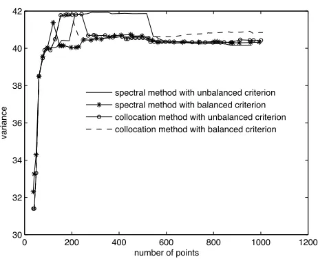
Figure 2. Convergence of the stochastic spectral and collocation methods using balanced and unbalanced criterions.
the new nodes. This approach can be seen as an adaptive building of the polynomial chaos.
Figure 2 shows the convergence study of the stochastic spectral method. Two criteria have been experimented in the adaptive algorithm: first, only the contribution of an index to the variance is considered; second, the contribution of an index to the variance is balanced by the number of new nodes to calculate, i.e., the computing time cost of the new nodes is taken into account. It appears that the convergence is better when using the balanced variance criterion: in this case, the variance converges after about 150 nodes while it needs more than 400 nodes in the case of the unbalanced criterion. The variance converges to a value close to the result obtained with the kriging technique (see Table 4). However, the stochastic method gives
Table 4. Mean and variance computed using the different methods.
Method Kriging Stochastic Stochastic spectral collocation Nb. of nodes 40 100 150 1,000 160 1,000
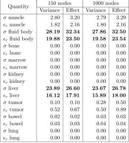
Table 5. Results for the stochastic spectral method: partial variance (%) and totaleffect (%) of the different parameters.
Quantity 150 nodes 1000 nodes Variance Effect Variance Effect
σ muscle 2.80 3.20 2.79 3.29
r muscle 1.82 2.16 1.80 2.16 σ fluid body 28.19 32.34 27.86 32.50
r fluid body 19.88 23.50 19.58 23.54
σ bone 0.00 0.00 0.00 0.00
r bone 0.00 0.00 0.00 0.00
σ marrow 0.00 0.00 0.00 0.00
r marrow 0.00 0.00 0.00 0.00 σ kidney 0.00 0.00 0.00 0.00
r kidney 0.00 0.00 0.00 0.00 σ liver 23.89 26.60 23.67 26.78
r liver 16.12 17.91 15.89 18.00 σ tumor 0.10 0.10 0.28 0.50
r tumor 0.52 0.67 0.50 0.89 σ bowel 0.02 0.02 0.03 0.03
r bowel 0.03 0.03 0.04 0.04
σ lung 0.00 0.00 0.00 0.00
r lung 0.00 0.00 0.00 0.00
a more accurate result with about one hundred nodes than the kriging method. The sensitivity analysis is reported in Table 5: the data are in agreement with those obtained by the kriging method. Three tissues impact on the variability ofy: the fluid body, the liver and the muscle. The others are nearly negligible and their influence is more residual than in the kriging prediction.
6. STOCHASTIC COLLOCATION METHOD
Stroud or Chebyshev nodes. As the sequences of nodes are nested, the error indicator on the value of y at new nodes can be given by the absolute difference with the values interpolated using the older nodes. In this section, we use the Matlab sparse grid interpolation toolbox [14]. As in the previous section, the adaptivity criterion can be or not be balanced by the numerical cost of a sequence. Both situations have been carried out and the results are given in Fig. 2. It appears that the results do not converge exactly to the same value: with 1,000 nodes, σ2y = 40.434 for the unbalanced criterion whereas
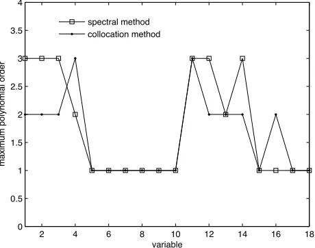
σy2 = 40.846 for the balanced one. The result with the unbalanced criterion is closer to the result given by the stochastic spectral method. Moreover, it seems that the convergence is achieved later compared to the stochastic spectralmethod. This is probably due to the fact that the collocation method adaptivity used here is related to the quality of the interpolation whereas the spectral method adaptivity is directly linked to the variance. The effect of the different strategies can also be viewed when one is interested in the maximum polynomial order reached in the 18 variables. Fig. 3 shows this result after 1,000 nodes for the spectral and collocation methods. In both cases, the most influential variables (number 1, 2, 3, 4, 11 and 12) are largely explored. The variables associated to the tumor properties (number 13 and 14) are also exploited because of their weaker but existing influence. However, the collocation method goes further in the exploration of the variable number 16 that corresponds to the bowel permittivity but this
2 4 6 8 10 12 14 16 18
0 0.5 1 1.5 2 2.5 3 3.5 4
variable
maximum polynomial order
spectral method collocation method
variable does not contribute to the variance as shown in Tables 3 and 5. Finally, the mean results are similar to the ones given by the spectral method (see Table 4).
7. CONCLUSION
The presence of uncertainties in the tissue properties has been analyzed in a 2D hyperthermia problem. Among the 18 uncertain properties, only those related to the tissues located in the neighborhood of the tumor have an impact on the repartition of the absorbed power. The sensitivity analysis made with fractional experimental designs leads to erroneous conclusions while the sensitivity and uncertainty analyses using the kriging technique give more accurate results. However, it appears that the spectralstochastic method is the best choice for this problem when it is used with an adaptive sparse grid algorithm: convergence is reached with about one hundred nodes. It has been shown that the implementation of the adaptative algorithm leads to an adaptative building of the polynomial chaos. On the contrary, using an adaptive sparse grid algorithm in a stochastic collocation method does not seem efficient but the reason is probably that the criterion for adaptivity used in this paper is not based on a statistical quantity; one should use a criterion based on the variance to improve the efficiency of the method. Finally, the 2D hyperthermia problem studied in this paper is usefulto properly compare different methods and the conclusions here can be straightforwardly extended to other situations.
APPENDIX A. AN ADAPTIVE VERSION OF SMOLYAK’S ALGORITHM IN STOCHASTIC PROBLEMS
Consider a regular univariate function f. The integralof f on the interval[−1,1] can be approximated by a quadrature formula of level
l:
1 −1
f(x)dx≈Ql(f) = nl
k=1
wl,kf(xl,k) (A1)
where the wl,k and xl,k are respectively the weights and the abscissas
tensor product of univariate quadrature formulas. Introducing the difference formulas:
∆l(f) =Ql(f)−Ql−1(f) withQ0(f) = 0, (A2) the conventional Smolyak algorithm to compute the integral of a d -variate functionF on the hypercube [−1,1]d is expressed by:
[−1,1]d
F(x)dx≈
j∈I(l)
⊗d k=1∆jk
(F) (A3)
withj= [j1, . . . , jd] andI(l) ={j| |j|1≤l−1}where|j|1 is the sum of
the componentsjk; thek-th componentjkis such thatjk+ 1 indicates
the level of accuracy of the quadrature rule following thek-th variable; the symbol ⊗dk=1∆jk denotes the tensor product of unidimensional
quadrature rules.
In the adaptative version of the algorithm, the summation in (A3) is extended to more generaladmissible sets than I(l). The only requirement for constructing these new admissible sets is that the difference formula ∆jk = Qjk − Qjk−1 can be computed. Thus, a
set of indices S is called admissible if, for all j ∈ S, j−ek ∈ S for
1≤k≤d; ek is thek-th unit vector [15]. Following this definition, a
generalsparse grid formula becomes:
[−1,1]d
F(x)dx≈
j∈S
⊗d k=1∆jk
(F) (A4)
withS a given admissible set.
The idea of the adaptative algorithm is then to construct nested sequences of admissible sets. This construction is performed by adding in priority, to already computed indexes, the indexes in the forward neighborhood of the index with the largest estimated error; the forward neighborhood of an index j is defined as the d indexes {j+ek |k= 1, . . . , d}. This leads to the desired dimension-adaptive
grid refinement. Newly added indexes are pooled as so-called active indexes while indexes of which the forward neighborhood has been processed becomeold indexes.
However, directly applying this algorithm in the case of the integrals of (4) needs some care. Each index j coincides with a maximum degree of functions that can be exactly integrated; since the integrand is of the form F = yΨi when evaluating yi, it implies
that an indexjenables to computeyi for a polynomial Ψiwhose degree
same direction: ik≤jk∀k. In other words, it means that as one moves
forward in the algorithm, that is to say as the number of indexesjfor which the nodes have been computed increases, the number of terms
yi that are estimated increases in the same way. Using the notations
given in [6], this specificity of the adaptative Smolyak algorithm is summarized in Algorithm 1. In this algorithm, O is the set of old indexes, A the set of active indexes, η the global error estimate, tol
the error tolerance andlindicates a truncation limit of the polynomial chaos.
Algorithm 2 is another solution: it is more substantial but requires more calculation.
Algorithm 1 Adaptative algorithm. Version 1.
yi=0 for i I(l)
j=[ 0,...,0]
for i I(l) do
yi =yi+ dk=1 jk (y i)
5: end for
O= A={j}
gj ; 2y =0
while ( tol) do
select j from Awith largestgj
10: A=A
O =O
for p=1,...,d do
h =j+ep
if h − eq O for all q=1,...,d then
15: A=A
fo i I(l) do
yi =yi+ dk=1 hk (y i)
end for
2
y, old = y2
20: y2= y2i withi O A\{[0 0]}
gh =
|
y2 y2,oldend if end for
25: end while
(
)
Ψ =+ =+ η \{j} {j} {h} Ψ(
)
|
−= max( )gj 2y withj A
Algorithm 2 Adaptativealgorithm. Version 2.
yi = 0 for i I(l)
j= [0, . . . ,0]
for i I(l) do
yi =yi+( kd=1 jk)(yΨi)
5: end for
O= A={j}
= + ;gj
while ( tol) do
select j from Awith largestgj 10: A =A \ {j}
O =O {j}
for p= 1,..., d do
h =j+ep
if h eq O for all q= 1,..., d then
15: A=A {h}
for i I(l) do
yi =yi+ dk=1 hk (yΨi)
end for end if
20: end for
AO+ =A O\ {[0 0]}
σ2
y = yi2 withi AO+
for j A do
for i AO+ \ j do
25: yi,tamp =yi dk=1 jk (y i)
end for
σ2
y,tamp = y2i with i AO+ \ j
gj = y2 y2,tamp
|
end for
30: = max gj 2y withj A
end while = +
|
( )∆
(
)
Ψ η ∞ − ε ⊗ ≥∈
∈
∈
∈
∈
∈
∈
⊗∈
⊗ ∪ ∆ ∞ ∪ σ σ ∆ − − ∪ η∈
σ / ) ( ∅; ,..., REFERENCES1. Hurt, W. D., J. M. Ziriax, and P. A. Mason, “Variability in EMF permittivity values: Implications for SAR calculations,” IEEE Trans. on Biomedical Engineering, Vol. 47, No. 3, 396–401, 2000. 2. Garcia-Diaz, A. and D. Philips,Principles of Experimental Design
and Analysis, Chapman & Hall, 1995.
Chapter Computer experiments, Elsevier Science, 1996.
4. Ghanem, R. G. and P. D. Spanos,Stochastic Finite Elements: A Spectral Approach, Springer-Verlag, New York, 1991.
5. Xiu, D. and J. S. Hesthaven, “High-order collocation methods for differentialequations with random inputs,”SIAM Journal on Scientific Computing, Vol. 27, No. 3, 1118–139, 2005.
6. Gerstner, T. and M. Griebel, “Dimension-adaptive tensor-product quadrature,” Computing, Vol. 71, No. 1, 65–87, Springer-Verlag, New York, Inc., 2003.
7. IFAC, Institute For Applied Physics, http://niremf.ifac.cnr.it/t-issprop/.
8. Stoneman, M. R., M. Kosempa, W. D. Gregory, C. W. Gregory, J. J. Marx, W. Mikkelson, J. Tjoe, and V. Raicu, “Correction of electrode polarization contributions to the dielectric properties of normaland cancerous breast tissues at audio/radiofrequencies,” Physical Medecine and Biology, Vol. 52, 6589–6604, 2007.
9. Renard, Y. and J. Pommier, “Getfem finite element library,” http://home.gna.org/getfem/.
10. OHagan, T. and M. Kennedy, “Gaussian emulator machine soft-ware,” http://www.tonyohagan.co.uk /academic/GEM/index.ht-ml.
11. Sobol, I. M., “Sensitivity estimates for non linear mathemati-calmodels,” Mathematical Modelling and Computational Experi-ments, Vol. 1, 407–14, 1993.
12. Xiu, D. and G. E. Karniadakis, “The Wiener-Askey polynomial chaos for stochastic differentialequations,” SIAM Journal on Scientific Computing, Vol. 24, No. 2, 619–44, (electronic), 2002. 13. Zeng, Z. Y. and J. M. Jin, “An efficient calculation of
scattering variation due to uncertain geometricaldeviation,” Electromagnetics, Vol. 27, No. 7, 387–398, 2007.
14. Klimke, A., “Sparse grid interpolation toolbox,” http://www.ia-ns.uni-stuttgart.de/spinterp/.