Comparing Different Schemes for Random Arrays
Giovanni Buonanno* and Raffaele Solimene
Abstract—In this work, four types of random arrays are compared. In particular, the mean and variance of the array factor are derived. This provides a partial statistical characterisation that allows pointing out some important aspects of random arrays and link them to the number of elements and array aperture. In the absence of a simple and effective analytical apparatus, here great importance is also given to the experimental aspect, especially as far as the side-lobe level is concerned. To this end, Monte Carlo simulations are run to experimentally build the side-lobe distribution as a function of the number of radiators and the average spacing between two adjacent radiators. The obtained results show that random arrays where one is free to impose constraints on the minimum spacing between adjacent elements can obtain performance analogous to those achievable by other schemes which do not put such constraints. However, the former are preferable because they are able to zero the probability that adjacent radiators are separated with less than a certain minimum distance, which allows the mitigation of mutual coupling effects.
1. INTRODUCTION
In aperiodic antenna arrays, the spacing between the elements is chosen to be incommensurable. This
distinctive feature offers a number of advantages as compared to equally-spaced arrays. Grating-lobes are in principle avoided according to nonuniform sampling theory [1, 2]. Hence, large scan angles are possible, and/or wide frequency ranges can be covered. This makes somehow the spatial non-uniformity as a synonymous of broadband functionality [3–5]. Again, especially for large aperture, the number of radiators can be reduced to a large extent without causing significant performance degradation, mainly as far as resolution is concerned. Accordingly, the average distance between adjacent radiators is increased, which makes the assumption of negligible mutual couplings more valid [6]. By reversing the perspective, having fixed the number of available radiators, they can be located on average more distant so to have an overall larger aperture. This in turn narrows the main-beam and hence leads to an improvement in resolution. Actually, the bandwidth-steerability product can be made much larger than for conventional equally-spaced arrays [5]. Finally, deploying the elements non-uniformly over the
array aperture allows the control of side-lobe level without the need to taper someway the excitation
currents. Accordingly, all the radiators can be uniformly excited so that the amplifiers can all work at maximum power, and this results in the simplification of the feeding network [7]. Actually, for aperiodic equally excited arrays the parameter that most influences the side-lobe level is the number of
radiators [6, 8]. Eventually, it can be stated that while designing aperiodic arrays one has more spatial
degrees of freedom allowed (i.e., all the positions of radiators instead of only the uniform step), and this in principle offers greater possibility for obtaining high performance arrays. Moreover, in many practical cases, the geometry of the array must necessarily be irregular [7].
Previous discussion justifies why aperiodic arrays have been the subject of a large body of research since long time [3, 8–14], and a number of ways to attack the analysis and synthesis of such a type of arrays have been proposed [15–25].
Received 10 August 2016, Accepted 7 November 2016, Scheduled 25 November 2016 * Corresponding author: Giovanni Buonanno ([email protected]).
In this paper, we focus on a special class of aperiodic array: the random arrays. Random arrays are those for which the positions of radiators are chosen according to some probabilistic law. This naturally leads to a nonuniform element arrangement (i.e., with probability one). The corresponding array factor
is thus a stochastic process whose features (if determined) allow for an a priori, though statistically,
performance analysis of this type of aperiodic arrays [26]. In this regard, the seminal paper of Lo [8] was the first at introducing a systematic theory of random arrays. Nonetheless, this issue is still an open problem. Indeed, while determining the array factor statistics up to the second order can be easily done, characterising the side-lobe level is a much harder problem. Actually, determining the side-lobe distribution requires finding that one of the supremum of the array factor magnitude. To cope with this problem the sampling [8, 27] and the level crossing approaches [28] are among the most used methods. More rigorously, the extreme value theory should be invoked [29]. However, this is not the subject of this paper.
In this paper, the aim is to compare different strategies for randomly generating the positions of radiators. In particular, we compare four types of positions generation rules while the elements are assumed to be equally-excited. Two approaches are borrowed from the array literature according to [8] and [30], respectively. Instead the other two approaches come from the nonuniform sampling theory [1]. For all the methods, the first (mean array factor) and second order (variance) statistics are analytically derived. The side-lobe level distribution is instead studied thanks to Montecarlo simulations.
2. RANDOM ARRAYS UNDER COMPARISON
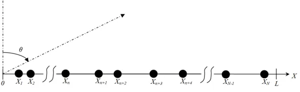
Consider a linear array ofN equally excited isotropic radiators placed at random along theX axis (see
Fig. 1). The corresponding (normalised) array factor can be written as [27]
F(u) = 1 N
N
n=1
ej2πXnu (1)
where
• u= sinθ−sinα;
• θis the observation angle from the broad-side;
• α is the scan angle;
• Xn is the location of the nth element normalised to the wavelength.
Figure 1. Generic random array where the positions of antenna elements are implicitly ordered.
The positions of radiators are randomly generated. Here, four types of generating rule are analysed.
The first generating rule leads to the so-called Totally Random Arrays (TRA) [8, 30]. Here, the
positions of antenna elements X1, X2, . . . , Xn are i.i.d. random variables with probability densities
supported over [0, L], Lbeing the length of the array normalised with respect to the wavelength.
The second generation rule is associated with the Binned Arrays (BA) [30] and can be expressed
as follows
Xn= (n−1)L
N +Yn n= 1,2, . . . , N (2)
whereinY1, Y2, . . . , YN are independent random variables each taking value within the interval [0, L/N].
The next rule is similar to the previous one [31, 32]
Xn= (n−1)(2ε+ Δ) +Wn n= 1,2, . . . , N (3)
where X1 = 0 and W1, W2, . . . , WN are independent random variables each assuming values in the
interval (−ε, ε), and Δ is a step parameter. This scheme is similar to some nonuniform sampling method
which is called periodic sampling with jitter [1]. For this reason, we address this way to generate random
arrays asJittered Random Arrays (JRA).
Finally, as a fourth rule the following scheme is considered [32]
Xn=Xn−1+Zn−1=
n−1
k=1
Zk n= 2, . . . , N (4)
in which X1 = 0 and Z1, Z2, . . . , ZN−1 are independent random variables taking values within the
interval [zmin, zmax]. Note that this is another rule used in nonuniform sampling theory which is
addressed as additive random sampling [1]. Accordingly, we address this random scheme as Additive
Random Arrays (ARA).
It is noted that these random arrays generally lead to different apertures. For example, the
maximum aperture for T RAs and BAs is L, for JRAs is [(2ε+ Δ)(N −1) + 2ε] while for ARAs
it is [(N −1)zmax]. The average distance between adjacent elements can be different as well as shown
below.
ForBAs, ifY1, Y2, . . . , YN arei.i.d.random variables, the average spacing between adjacent antenna
elements is
dav=E[Xn]−E[Xn−1] = (n−1)L
N +E[Yn]−(n−2) L
N −E[Yn−1] = L
N (5)
For JRAs, if W1, W2, . . . , WN are i.i.d. random variables, the average spacing between adjacent
radiators is
dav =E[Xn]−E[Xn−1] = (n−1)(2ε+ Δ) +E[Wn]−(n−2)(2ε+ Δ)−E[Wn−1] = (2ε+ Δ) (6)
For ARAs, if Z1, Z2, . . . , ZN are i.i.d. random variables, the average spacing between adjacent
antenna elements is
dav=E[Xn]−E[Xn−1] =E[Z] =
zmax
zmin
Z f(Z) dZ (7)
In the case ofT RAs, the element positions are not in general ordered. However, one can resort to
the order statistics [33] by putting
X(1) = min(X1, X2, X3, . . . , XN)
X(2) = min({X1, X2, X3, . . . , XN} − {X(1)})
.. .
X(n) = min({X1, X2, X3, . . . , XN} − {X(1), X(2), . . . , X(n−1)})
.. .
X(N) = Max(X1, X2, X3, . . . , XN)
(8)
so thatX(1) ≤X(2) ≤. . .≤X(n) ≤. . .≤X(N). X(n)is called thenth order statistics whose distribution,
since the positions arei.i.d., is given as [33]
fn(x) = N
!
(n−1)!(N−n)!F
n−1(
x)[1−F(x)]N−nf(x) (9)
where F(x) and f(x) are the cumulative distribution function (CDF) and the probability density
function (P DF) of the above positions, respectively. If θp is thepth quantile of the common CDF of
the positions of radiators and f(θp)= 0, then follows that [34]
E[X(n)]≈θp, p= n
So, in general,E[X(n)]−E[X(n−1)]=E[X(m)]−E[X(m−1)], but for uniform distribution
E[X(n)]−E[X(n−1)] =
L
N + 1 ∀n (11)
and then this quantity can be identified as the average spacing, dav, between adjacent radiators†.
Looking at Eqs. (7)–(11), one can also observe that forBAsandJRAsthe average spacing between
adjacent antenna elements does not depend on the probability distribution, as instead it is for T RAs
and ARAs. It is also important to remark that while for T RAs and BAs the radiators can be placed
at each point within the aperture, no matter how close they are, this does not hold true forARAsand
JRAs. Indeed, in BAs two consecutive elements could result in coincidence whereas in T RAs even
all the elements could in principle be located at the same position. Instead for ARAs, the distance
between adjacent radiators cannot be smaller thanzmin while inJRAsthere are points on the aperture
where none antenna element can be placed, i.e., those points that fall within the Δ intervals cannot
accommodate any location of radiators. From the point of view of mutual coupling, with JRAs and
ARAsone can constraint the minimum distance between two adjacent antenna elements. For example,
ifd is the minimum acceptable spacing between adjacent radiators, then forJRAs one can set Δ≥d
whereas for ARAs,zmin =d.
3. FIRST AND SECOND ORDER CHARACTERISATION
A useful even though partial statistical characterisation of the random arrays (obtained according to the rules reported above) can be easily given. Therefore, here, we derive the mean and variance of the array factors under comparison.
We start with theT RAs. In this case, the mean and variance of the array factor are the following
φT RA(u) =E[F(u)] =
L
0
f(X) ej2πXudX =ψX(u) (12)
and
σT RA2 (u) = E[|F(u)−φT RA(u)|2] =E[|F(u)|2]− |φT RA(u)|2
= E
1 N
N
n=1
ej2πXnu· 1 N
N
m=1
e−j2πXmu
− |φT RA(u)|2
= 1
N2
N
n=1
N
m=1
Eej2πXnu·e−j2πXmu− |φ
T RA(u)|2
= 1
N +
N
n=1
N
m=1
m=n
Eej2πXnu·Ee−j2πXmu− |φ
T RA(u)|2 =
1− |φT RA(u)|2
N (13)
For BAs, if Y1, Y2, . . . , YN are i.i.d. random variables, the mean and variance of the array factor
are
φBA(u) =
1 N
N
n=1
ej2π(n−1)NLu·Eej2πYnu = e
−j2πNLu
N ·ψY(u)·
N
n=1
ej2πnNLu
= e
jπLNN−1u
N ·ψY(u)·
sin (πLu)
sinπNLu (14)
whereas
σ2BA(u) =
1 N2 N n=1 N m=1
ej2π(n−m)NLuEej2πYnu·e−j2πYmu− |φBA(u)|2
= 1
N +
1
N2 |ψY(u)| 2N
n=1
N
m=1
m=n
ej2π(n−m)NLu− |φBA(u)|2 = 1− |ψY(u)|
2
N (15)
whereψY(u) =E
ej2πY u=0L/Nf(Y)·ej2πY udY is once again the characteristic function associated
to the random variable Y.
Similar results are obtained for JRAs after assuming, as done above, that W1, W2, . . . , WN are
i.i.d. random variables. Accordingly, the mean and variance of the array factor are
φJRA(u) =
1 N N n=1
ej2π(n−1)(2ε+Δ)u·Eej2πWnu = e
−j2π(2ε+Δ)u
N ·ψW(u)·
N
n=1
ej2πn(2ε+Δ)u
= e
jπ(N−1)(2ε+Δ)u
N ·ψW(u)·
sin[πN(2ε+ Δ)u]
sin[π(2ε+ Δ)u] (16)
and
σJRA2 (u) =
1 N2 N n=1 N m=1
ej2π(n−m)(2ε+Δ)u·Eej2πWnu·e−j2πWmu− |φJRA(u)|2
= 1
N +
|ψW(u)|2
N2 ·
N n=1 N m=1
m=n
ej2π(n−m)(2ε+Δ)u− |φJRA(u)|2 =
1− |ψW(u)|2
N (17)
withψW(u) =E
ej2πW u=−εεf(W)·ej2πW udW.
Finally, for ARAs, if Z1, Z2, . . . , ZN−1 are as usuali.i.d. random variables, we get
φARA(u) =
1 N · N n=1 E
ej2πnk=1−1Zku= 1
N ·
N
n=1
Eej2πZu(n−1) = 1
N ·
N
n=1
ψZ(u)(n−1) (18)
and
σARA2 (u) =
1 N2 N n=1 N m=1
Eej2πXnu·e−j2πXmu− |φARA(u)|2
= 1 N + 1 N2 N n=1 N m=1
m=n
Eej2πXnu·e−j2πXmu− |φARA(u)|2
= 1 N + 1 N2 N n=1 N m=1
m=n
E
ej2πnk=1−1Zku·e−j2πmp=1−1Zpu− |
φARA(u)|2
= 1
N − |φARA(u)|
2+ 1
N2 N n=1 N m=1 m<n E
ej2πnk=1−1Zku·e−j2πmp=1−1Zpu
+ 1 N2 N n=1 N m=1 m>n E
ej2πnk−=11Zku·e−j2πmp=1−1Zpu
= 1
N − |φARA(u)|
2+ 1
N2 N n=1 N m=1 m<n
ψZ(u)(n−m)+
1 N2 N n=1 N m=1 m>n
withψZ(u) =E{ej2πZu}=
zmax
zmin f(Z)·e
j2πZudZ.
The central role played by the characteristic functions must be noted.
In order to perform a comparison, we take the same cases as addressed in [30]. The array consists
of 100 radiators and has nominal aperture of 400λ. For JRA and ARA, we can set the minimum
acceptable distance between adjacent elements. According to common usage for avoiding mutual
coupling, this distance is chosen equal to λ/2. Therefore, Δ = 1/2 and zmin = 1/2, respectively.
Moreover, since the nominal aperture is 400λ, ε = 1.7525 and zmax = 4.0404 for JRA and ARA,
respectively. Furthermore, forT RA, the variablesX1, X2, . . . , XN are chosen to be uniformly distributed
within [0, L]; for BA, the variables Y1, Y2, . . . , YN are uniformly distributed within [0, L/N]; for JRA,
the variablesW1, W2, . . . , WN are uniformly distributed within [−ε, ε], and finally forARA, the variables
Z1, Z2, . . . , ZN−1 are uniformly distributed within [zmin, zmax]. This way, the mean array factors are
specialised as
φT RA(u) = φBA(u) =ejπLu·
sin(πLu)
πLu (20)
φJRA(u) = e
jπ(N−1)(2ε+Δ)u
N ·
sin(2πεu)
2πεu ·
sin[πN(2ε+ Δ)u]
sin[π(2ε+ Δ)u] (21)
φARA(u) =
1
N ·
N
n=1
ej2πzmaxu−ej2πzminu
j2π(zmax−zmin)u
n−1
(22)
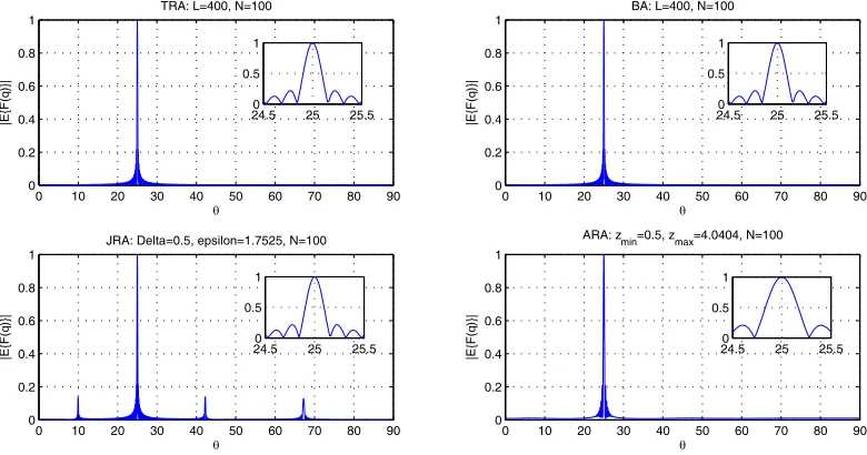
In Fig. 2, the magnitude of such mean array factors is reported as a function of the observation angle θhaving fixed the steering angle atα= 25◦. As can be seen,|E{F(u)}|forT RAand BAare identical
and similar to that of a continuous uniform current distribution. ForJRA, the magnitude of the mean
array factor is similar to the two previous ones around the main beam region, say forθ approximately
within (10◦,40◦). However, it presents small peaks in correspondence of θ = sin−1[−(1/(2ε+ Δ)) + sin(θ0)]≈9.96◦,θ= sin−1[(1/(2ε+Δ))+sin(θ0)]≈42.24◦andθ= sin−1[(2/(2ε+Δ))+sin(θ0)]≈67.22◦
which are due to the periodic function{sin[πN(2ε+ Δ)u]/sin[π(2ε+ Δ)u]}. Moreover, forθaway from all peaks, owing to the function {sin(2πεu)/(2πεu)} the level is lower than φT RA(u). It is noted that
in order to remedy the presence of the small peaks, one might think to synthesiseP DF of the random
variables W1, W2, . . . , WN so as to have zeros just in correspondence of such peak positions. Finally,
for ARAs the magnitude of the mean array factor is still similar to the previous ones up to the first
side-lobe region, which is close to the main lobe. Away from that region, however, it does not tend to
0 10 20 30 40 50 60 70 80 90
0 0.2 0.4 0.6 0.8 1
TRA: L=400, N=100
θ
|E{F(
q
)}|
0 10 20 30 40 50 60 70 80 90
0 0.2 0.4 0.6 0.8 1
|E{F(
q
)}|
θ BA: L=400, N=100
0 10 20 30 40 50 60 70 80 90
0 0.2 0.4 0.6 0.8 1
|E{F(
q
)}|
θ
JRA: Delta=0.5, epsilon=1.7525, N=100
0 10 20 30 40 50 60 70 80 90
0 0.2 0.4 0.6 0.8 1
|E{F(
q
)}|
θ
ARA: zmin=0.5, zmax=4.0404, N=100 24.50 25 25.5 0.5
1
24.50 25 25.5 0.5
1
24.50 25 25.5 0.5
1
24.50 25 25.5 0.5
1
0 10 20 30 40 50 60 70 80 90 0
0.2 0.4 0.6 0.8 1
TRA: L=400, N=100
θ 0 10 20 30 40 50 60 70 80 90
0 0.2 0.4 0.6 0.8 1
BA: L=400, N=100
θ
0 10 20 30 40 50 60 70 80 90
0 0.2 0.4 0.6 0.8 1
JRA: Delta=0.5, epsilon=1.7525, N=100
θ 0 10 20 30 40 50 60 70 80 90
0 0.2 0.4 0.6 0.8 1
ARA: zmin=0.5, zmax=4.0404, N=100
θ
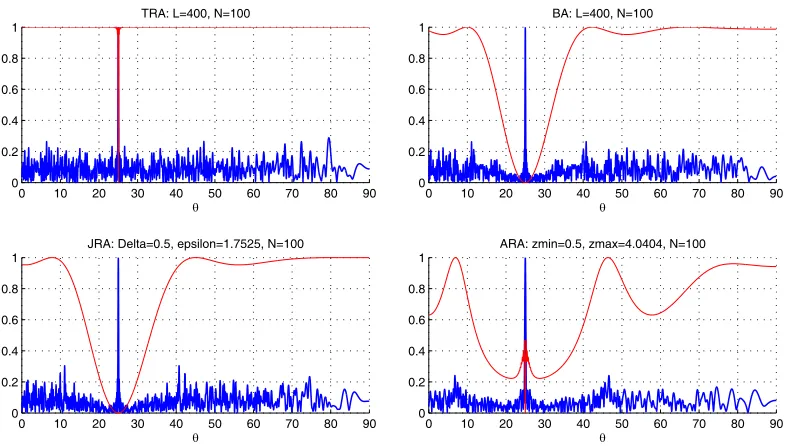
Figure 3. Magnitude of sample array factors (blue lines) with normalised variances (red lines) superimposed. The parameters are the same as in Fig. 2.
zero but assumes a nearly constant value.
In Fig. 3, sample functions of the array factor magnitude for the different cases under consideration are shown (blue lines) along with the corresponding normalised variance (red lines) defined as ˜σi2(u) =
σ2
i(u)/maxu{σi2(u)} withi=T RA, BA, JRA, ARA. As already shown in [30], the variance relative to
BAis considerably slower at reaching its maximum thanT RA. A slightly slower behaviour is observed
forJRAwhile the slowest to achieve the variance maximum, even though with an oscillatory trend, are
ARAs. However, the latter exhibit higher variance values close to the main beam.
Within the region where the variance assumes low value, the array factor is more probable to be
similar to the mean one. Therefore, at least for T RAs,BAs and JRAs, it can be concluded that the
array factor around the main-beam region is practically certain to coincide with the mean one. This
statement basically coincides with the claim that resolution is mainly affected by the array aperture
rather than by the number and the way the elements are deployed. Moreover, in this regard BAs and
JRAshave a largecertain region (as the variance grows up more slowly) and hence should be preferred.
Finally, it is remarked that previous discussion does not dependent on the steering angle.
4. SIDE-LOBE LEVEL
In this section, we turn to consider the comparison in terms of the the side-lobe level (SLL). TheSLL
is defined as
SLL= max
u∈[δ,2]|F(u)| (23)
withδ >0 being the point where the side-lobe region starts. According to the previous discussion about
the almost deterministic nature of the main beam,δ can be directly linked to the reciprocal of the array
aperture. In particular, it can be fixed as the first zero of the mean array factor. Only the interval [δ,2]
is of concern. This is because the array factor magnitude is an even function. Also, limiting u to be
≤2 allows covering all the visible domain, whatever the steering angle is.
According to Eq. (23), in order to perform the study, the statistical characterisation of maxu∈[δ,2]|F(u)| is required. This is a hard task which in general cannot be solved in closed form. To cope with this problem, some approximate approaches have been proposed in literature [8, 27– 29, 35]. Here, the main focus is on establishing how the different random arrays perform. To this
corresponding distributions by Monte Carlo simulations (20000 trials indeed). More in details, in order to highlight the role played by different array settings, different average spacings dAV = 1/2,1,2.5,5
(between adjacent) antenna elements are considered. Also the number of radiators, for each value of
the average spacing, is varied from 20 to 200 with a step of 20. For JRAs and ARAs, the minimum
acceptable spacing between adjacent antenna elements is chosen equal to 0.3 for dAV = 1/2, while it is
chosen equal to 1/2 for the other values of dAV. Finally, while performing the simulations, the array
factor magnitude is sampled at a step equal to the reciprocal of 20 times the maximum array aperture, which is a much finer step than the one usually used while analysing this kind of arrays [27].
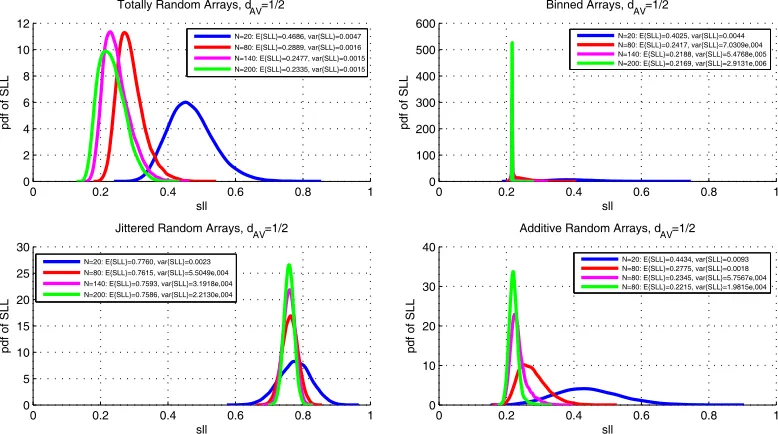
In Fig. 4, the experimentalSLLdistributions are reported for dav = 1/2 and for different numbers
N of elements. Note that keeping fixed dav while increasingN entails increasing the array aperture as
well. First, it can be observed that asN increases all the distributions tend to be more peaked. This is
somehow consistent with the behaviour of the variances asN increases reported in the previous section.
Indeed, when N increases, in all the schemes under consideration, the variance decreases making it
thus natural to expect that the SLL approaches the one corresponding to the average array factor.
It is seen that JRAs have a rather high SLL as compared to the other schemes. This is clearly due
to the Dirichlet sine term sin[πN(2ε+ Δ)u]/sin[π(2ε+ Δ)u] which is responsible for greeting lobes
appearing at u = 2. Actually, this holds true as long as dav does not exceed 1. Indeed, when dAV is
low and Δ comparable with it, ε is small as well. Hence, the perturbation (on the deterministic parts
of the positions of radiators) (n−1)(2ε+ Δ) withn= 1,2, . . . , N, is negligible. On the contrary, when
the average spacing is high, and hence ε can assume sufficiently great values, the JRAs performance
becomes similar to those of the other methods.
That figure also shows that when it is allowed to use an average spacing equal toλ/2, random arrays
generally return a worse SLL than the usual uniform arrays. However, it is interesting to note that
asN increases the SLL tends (even though differently for each scheme but theJRA) to the standard
−13 dB of uniform arrays, regardless the way the elements are arranged over the aperture.
We now turn to address the case reported in Fig. 5 where dav is increased up to 5. It can be
observed that the trend highlighted while discussing the previous figure still persists. Furthermore, as
anticipated before, now JRAs are no more affected by high SLL, and their P DF are similar to the
ones of BAs.
It must be remarked that now the number of elements is roughly ten times lower than the one that should be used under a uniform setting. This entails that if uniform arrays were used a number of greeting lobes would manifest. Hence, the advantage provided by randomly putting the radiating
0 0.2 0.4 0.6 0.8 1
0 2 4 6 8 10 12
Totally Random Arrays, d
AV=1/2
pdf of SLL
sll
0 0.2 0.4 0.6 0.8 1
0 100 200 300 400 500 600
Binned Arrays, d
AV=1/2
pdf of SLL
sll
0 0.2 0.4 0.6 0.8 1
0 5 10 15 20 25 30
Jittered Random Arrays, d
AV=1/2
pdf of SLL
sll
0 0.2 0.4 0.6 0.8 1
0 10 20 30 40
Additive Random Arrays, d
AV=1/2
pdf of SLL
sll
N=20: E{SLL}=0.4686, var{SLL}=0.0047 N=80: E{SLL}=0.2889, var{SLL}=0.0016 N=140: E{SLL}=0.2477, var{SLL}=0.0015 N=200: E{SLL}=0.2335, var{SLL}=0.0015
N=20: E{SLL}=0.4025, var{SLL}=0.0044 N=80: E{SLL}=0.2417, var{SLL}=7.0309e,004 N=140: E{SLL}=0.2188, var{SLL}=5.4768e,005 N=200: E{SLL}=0.2169, var{SLL}=2.9131e,006
N=20: E{SLL}=0.7760, var{SLL}=0.0023 N=80: E{SLL}=0.7615, var{SLL}=5.5049e,004 N=140: E{SLL}=0.7593, var{SLL}=3.1918e,004 N=200: E{SLL}=0.7586, var{SLL}=2.2130e,004
N=20: E{SLL}=0.4434, var{SLL}=0.0093 N=80: E{SLL}=0.2775, var{SLL}=0.0018 N=80: E{SLL}=0.2345, var{SLL}=5.7567e,004 N=80: E{SLL}=0.2215, var{SLL}=1.9815e,004
0 0.2 0.4 0.6 0.8 1 0
5 10 15 20
sll
pdf of SLL
Totally Random Arrays, d
AV=5
0 0.2 0.4 0.6 0.8 1
0 100 200 300 400
sll Binned Arrays, d
AV=5
pdf of SLL
0 0.2 0.4 0.6 0.8 1
0 100 200 300 400 500
sll Jittered Random Arrays, d
AV=5
pdf of SLL
0 0.2 0.4 0.6 0.8 1
0 5 10 15 20 25
sll Additive Random Arrays, d
AV=5
pdf of SLL
N=20: E{SLL}=0.5694, var{SLL}=0.0024 N=80: E{SLL}=0.3251, var{SLL}=8.2686e*004 N=140: E{SLL}=0.2651, var{SLL}=8.3648e*004 N=200: E{SLL}=0.2407, var{SLL}=0.0010
N=20: E{SLL}=0.5649, var{SLL}=0.0023 N=80: E{SLL}=0.3171, var{SLL}=5.8852e*004 N=140: E{SLL}=0.2490, var{SLL}=3.2542e*004 N=200: E{SLL}=0.2211, var{SLL}=7.9381e*005
N=20: E{SLL}=0.5654, var{SLL}=0.0023 N=80: E{SLL}=0.3183, var{SLL}=6.0667e*004 N=140: E{SLL}=0.2506, var{SLL}=3.4654e*004 N=200: E{SLL}=0.2223, var{SLL}=1.0818e*004
N=20: E{SLL}=0.5638, var{SLL}=0.0023 N=80: E{SLL}=0.3174, var{SLL}=5.9577e*004 N=140: E{SLL}=0.2528, var{SLL}=3.3839e*004 N=200: E{SLL}=0.2280, var{SLL}=3.4869e*004
Figure 5. SLLdistributions as a function of the number of antenna elements with dav set at 5.
20 40 60 80 100 120 140 160 180 200
0.2 0.4 0.6 0.8 1
d
AV=1/2
N
max{SLL}
20 40 60 80 100 120 140 160 180 200
0.2 0.4 0.6 0.8 1
d
AV=1
N
max{SLL}
20 40 60 80 100 120 140 160 180 200
0.2 0.4 0.6 0.8 1
dAV=2.5
N
max{SLL}
20 40 60 80 100 120 140 160 180 200
0.2 0.4 0.6 0.8 1
dAV=5
N
max{SLL}
TRAs BAs JRAs ARAs
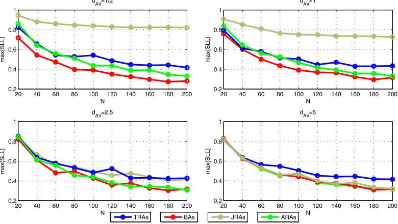
Figure 6. Statistical maximum of theSLLfor each type of array as function of the number of antenna elements and for diferent average spacing.
elements is evident, especially when N increases. Moreover, by comparing Figs. 4 and 5 once again it
is clear that the most important parameter that governs theSLL is the number of radiators and much
less the array aperture. Indeed, theSLLdistributions corresponding to the sameN but at differentdav
are very similar (of course, leaving outside the discussion JRAs as explained above) even though the
same number of radiators is deployed over two different array apertures (i.e, the second aperture is ten
times larger than the first one). Instead, according to the previous discussion, for JRAs, the aperture
also plays a crucial role. However, when a large array aperture is of concernJRAsshould be preferred.
This is because theSLLdistribution is as peaked asBAs P DF, but JRAsalso allow constraint of the
distance between adjacent radiators and hence someway mitigation of mutual coupling.
(i.e., the lower and upper edges of the support of the SLL distributions) are compared. These curves
are basically a measure of the best and worst cases as far as SLLis concerned. Indeed, having fixedN
anddav, the probability that theSLLis below the maximum one is 1. Therefore, even by only one trial,
it is almost sure that the sample array factor hasSLL below the experimental max{SLL}. Also, from
Fig. 6 it can be seen thatBAs are generally the best. Furthermore, as expected, for low values of dAv,
JRAs have very high SLL. However, when the average spacing is increased, JRAs behave similarly
to the other methods. Also, as remarked above, they should be preferred to BAs for mutual coupling
reason, and with respect the other two methods becauseP DF is more peaked around the mean.
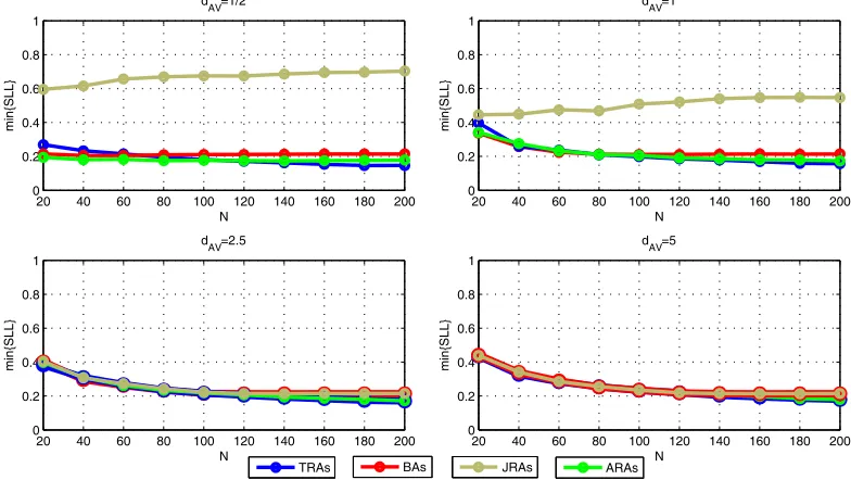
Finally, Fig. 7 compares the experimental statistical minimum curves of the SLL. These curves
can be used as a reference for the best achievable case, although to obtain the optimal positions, i.e.,
the one that provides such minimum SLL, one in general needs to generate many sample positions
vectors. As may be observed, T RAs and ARAs are slightly better (this is already evident in Figs. 4
and 5 indeed). However, according to previous discussion, JRAs are still preferable. It is interesting
to note that, although for dAV = 1/2 random arrays give in general highSLL as compared to uniform
arrays, there is at least one random configuration (the one corresponding to the minimum SLL) that
can return a SLL slightly below the standard −13.4 dB. In this regard, when radiators are equally
excited randomising their locations can lead to lower SLL, confirming what reported in the classical
paper [4].
20 40 60 80 100 120 140 160 180 200
0 0.2 0.4 0.6 0.8 1
d
AV=1/2
N
min{SLL}
20 40 60 80 100 120 140 160 180 200
0 0.2 0.4 0.6 0.8 1
d
AV=1
N
min{SLL}
20 40 60 80 100 120 140 160 180 200
0 0.2 0.4 0.6 0.8 1
dAV=2.5
N
min{SLL}
20 40 60 80 100 120 140 160 180 200
0 0.2 0.4 0.6 0.8 1
dAV=5
N
min{SLL}
TRAs BAs JRAs ARAs
Figure 7. Statistical minimum of theSLLfor each type of array as function of the number of antenna elements and for different average spacing.
5. CONCLUSIONS
In this work, four different rules for randomly generating the positions of radiators in random arrays
are compared. In particular, we bring together approaches coming from antenna arrays literature
(i.e., T RAs and BAs) and nonuniform sampling theory (i.e., JRAs and ARAs). The two worlds are
naturally linked when the positions of antenna elements are replaced by the sampling points although the applications and specifications to be met could be generally different.
For each generation rule, the mean and variance of the array factor are provided under the
assumption (rather common indeed) the random variables describing the element positions are i.i.d..
The side-lobe distribution is worked out via a Monte Carlo analysis. It is shown that for low values
of average spacing between antenna elements, BAa and ARAs are the better ones and have similar
performance. However, the latter have the advantage of being able to fix a minimum distance allowed
between adjacent elements and hence counteract mutual coupling effects. For high values ofdav,JRAs
become more convenient. In particular, they exhibit performance similar to BAs but more resilient
to mutual coupling effects. Furthermore, JRAs are also interesting because they can be optimised by
simply controlling the deterministic parameters, εand Δ [31].
We end this paper by observing that even thoughT RAshave the worse performance (at least from
theSLLpoint of view that was of main concern herein) they can be analytically studied with less effort
also from the synthesis point of view. More in detail, as the larger the number of radiators the smaller the variance (this is actually holds true for all the generating schemes), the array factor resembles more
and more the mean array factor. Hence, for a sufficiently highN, the synthesis of the array factor may
be re-phrased as the synthesis of the mean array factor, which in turn is linked to the position P DF
the same way the far-field pattern is related to a continuous line-source [36]. Therefore, one can set the
array factor according to some assigned pattern (not just the main beam width and/or the SLL) and
find the correspondingP DF. We plan to show this approach in a future paper.
REFERENCES
1. Bilinskis, I., Digital Alias-free Signal Processing, John Wiley & Sons, Inc., 2007.
2. Holm, S., A. Austeng, K. Iranpour, and J. F. Hopperstad, “Nonuniform sampling: Theory and
practice,”F. Marvasti Nonuniform Sampling: Theory and Practice, Chapter 19, 2001.
3. King, D. D., R. F. Packard, and R. K. Thomas, “Unequally-spaced, broad-band antenna arrays,”
IRE Trans. Antennas Propagat., Vol. 8, 380–384, 1960.
4. Ishimaru, A. and Y. S. Chen, “Thinning and broadbanding antenna arrays by unequal spacings,”
IEEE Trans. Antennas Propagat., Vol. 13, 34–42, January 1965.
5. Andreasen, M. G., “Linear arrays with variable in-terelement spacing,” IRE Trans. Antennas
Propagat., Vol. 10, 137–143, 1962.
6. Steinberg, B. D., “The peak sidelobe of the phased array having randomly located elements,”IEEE
Trans. Antennas Propagat., Vol. 20, 129–136, 1972.
7. Leahy, B. D. and B. D. Jeffs, “On the design of maximally sparse beamforming arrays,” IEEE
Trans. Antennas Propagat., Vol. 39, No. 8, 1178–1187, 1991.
8. Lo, Y. T., “A mathematical theory of antenna arrays with randomly spaced elements,”IEEE Trans.
Antennas Propagat., Vol. 12, 257268, 1964.
9. Unz, H., “Linear arrays with arbitrarily distributed elements,” IRE Trans. Antennas Propagat.,
Vol. 8, 222–223, 1960.
10. Ishimaru, A., “Theory of unequally-spaced arrays,”IRE Trans. Antennas Propagat., Vol. 10, 691–
702, 1962.
11. Willey, R. E., “Space tapering of linear and planar arrays,”IEEE Trans. Antennas Propag., Vol. 10,
No. 4, 369–377, 1962.
12. Sandler, S., “Some equivalences between equally and unequally spaced arrays,” IRE Trans.
Antennas Propagat., Vol. 8, 496–500, September 1960.
13. Maffett, A. L., “Array factors with non uniform spacing parameters,” IRE Trans. Antennas
Propagat., Vol. 10, 131–146, 1962.
14. Skolnik, M., G. Nemhauser, and J. Sherman “Dynamic programming applied to unequally spaced
arrays,” IEEE Trans. Antennas Propag., 35–43, January 1964.
15. Skolnik, M. I., J. W. Sherman III, and F. C. Ogg, Jr., “Statistically designed density-tapered
arrays,” IEEE Trans. Antennas Propag., Vol. 12, 408–417, July 1964.
16. Haupt, R. L., “Thinned arrays using genetic algorithms,”IEEE Trans. Antennas Propag., Vol. 42,
No. 7, 993–999 1994.
17. Haupt, R. L., “Unit circle representation of aperiodic arrays,” IEEE Trans. Antennas Propag.,
18. Kerby, K. C. and J. T. Bernhard, “Sidelobe level and wideband behavior of arrays of random
subarrays,” IEEE Trans. Antennas Propag., Vol. 54, No. 8, 2253–2262, 2006.
19. Liu, Y., Z.-P. Nie, and Q. H. Liu, “A new method for the synthesis of non-uniform linear arrays
with shaped power patterns,”Progress In Electromagnetics Research, Vol. 107, 349–363, 2010.
20. Zhao, X., Q. Yang, and Y. Zhang, “Compressed sensing approach for pattern synthesis of maximally
sparse non-uniform linear array,” IET Microw., Antennas Propag., Vol. 8, No. 5, 301–307, 2013.
21. Gregory, M. and D. Werner, “Ultrawideband aperiodic antenna arrays based on optimized raised
power series representations,” IEEE Trans. Antennas Propag., Vol. 58, No. 3, 756–764 2010.
22. Tokan, F. and F. Gunes, “The multi-objective optimization of non-uniform linear phased arrays
using the genetic algorithm,” Progress In Electromagnetics Research B, Vol. 17, 135–151, 2009.
23. Razavi, A. and K. Forooraghi, “Thinned arrays using pattern search algorithms,” Progress In
Electromagnetics Research, Vol. 78, 61–71, 2008.
24. Kumar, B. P. and G. R. Branner, “Synthesis of unequally spaced arrays using Legendre series
expansion,” Proc. IEEE Antennas Propag. Int. Symp., Vol. 4, 2236–2239, 1997.
25. Kurup, D. G., M. Himdi, and A. Rydberg, “Synthesis of uniform amplitude unequally spaced
antenna arrays using the differential evolution algorithm,”IEEE Trans. Antennas Propag., Vol. 51,
2210–2217, 2003.
26. Lo, Y. T. and S. W. Lee, “Aperiod arrays,” Chapman and Hall, Antenna Handbook: Antenna
Theory, Vol. 2, Chapter 14, 1993.
27. Agrawal, V. and Y. Lo, “Distribution of sidelobe level in random arrays,” Proc. IEEE, Vol. 57,
No. 10, 1764–1765, 1969.
28. Donvito, M. B. and S. A. Kassam, “Characterization of the random array peak sidelobe,” IEEE
Trans. Antennas Propagat., Vol. 27, 379–385, May 1979.
29. Krishnamurthy, S., D. Bliss, C. Richmond, V. Tarokh, “Peak sidelobe level gumbel distribution
for arrays of randomly placed antennas,” 2015 IEEE National Radar Conference — Proceedings,
1671–1676, 2015.
30. Hendricks, W. J., “The totally random versus the bin approach for random arrays,” IEEE Trans.
Antennas Propag., Vol. 39, 1757–1762, 1991.
31. Shinohara, N., B. Shishkov, H. Matsumoto, K. Hashimoto, and A. K. M. Baki, “New stochastic algorithm for optimization of both side lobes and grating lobes in large antenna arrays for MPT,”
IEICE Transactions on Communications, Vol. 91-B, No. 1, 286–296, 2008.
32. Kolghi, H. and S. B. Kesler, “Comparison of two methods of generating sensor locations in random
array,”Antennas and Propagation Society International Symposium, Vol. 24, 1986.
33. Papoulis, A. and S. U. Pillai,Probability, Random Variables and Stochastic Processes, 4th Edition,
McGraw Hill, 2002.
34. Baglivo, J. A.,Mathematica Laboratories for Mathematical Statistics, Emphasizing Simulation and
Computer Intensive Methods, ASA-SIAM, Chapter 9, 120, 2005.
35. Agrawal, V. D. and Y. T. Lo, “Mutual coupling in phased arrays of randomly spaced antennas,”
IEEE Trans. on Antennas and Propagat, Vol. 20, 288–295, 1972.
36. Balanis, C. A., Antenna Theory: Analysis and Design, 2nd Edition, John Wiley and Sons, Inc.,