Design and Simulation of Arbitrarily-Shaped Transformation Optic
Devices Using a Simple Finite-Difference Method
Eric A. Berry, Jesus J. Gutierrez, and Raymond C. Rumpf*
Abstract—A fast and simple design methodology for transformation optics (TO) is described for devices having completely arbitrary geometries. An intuitive approach to the design of arbitrary devices is presented which enables possibilities not available through analytical coordinate transformations. Laplace’s equation is solved using the finite-difference method to generate the arbitrary spatial transforms. Simple techniques are presented for enforcing boundary conditions and for isolating the solution of Laplace’s equation to just the device itself. It is then described how to calculate the permittivity and permeability functions via TO from the numerical spatial transforms. Last, a modification is made to the standard anisotropic finite-difference frequency-domain (AFDFD) method for much faster and more efficient simulations. Several examples are given at the end to benchmark and to demonstrate the versatility of the approach. This work provides the basis for a complete set of tools to design and simulate TO devices of any shape and size.
1. INTRODUCTION
Transformation optics (TO) is a design methodology that allows electromagnetic fields to be controlled through spatial transforms [1]. The most well-known example is the cylindrical electromagnetic cloak described in Ref. [2]. Their device used a form expression for the spatial transform, but closed-form expressions are highly limited in the range of geometries they can describe. In order to design an arbitrarily shaped device using TO, a fully numerical method is necessary to perform the coordinate transformation and to calculate the resulting material properties for the device. This paper presents a fully numerical technique based on the finite-difference method to generate and simulate arbitrary TO devices. The arbitrary spatial transforms are generated numerically by solving Laplace’s equation [3, 4]. The devices are confirmed through simulation using an improved anisotropic finite-difference frequency-domain (AFDFD) method [5] that more efficiently simulates waves in arbitrary anisotropic media. Several examples are given to demonstrate the simplicity and versatility of our approach. This is the first known description of a complete numerical tool chain for TO that is based on the finite-difference method.
Historically, methods such as quasi-conformal mapping [6] and the solution of various partial differential equations such as Laplace’s equation [3, 4], Poisson’s equation [7], and the Helmholtz equation [8] have been used to generate the TO material parameters numerically. The approach presented in Ref. [6] can create arbitrary dielectric waveguides using TO, but does not allow for devices such as cloaks and lenses to be designed. The techniques described in Refs. [3, 4, 7, 8] use a commercial finite element software such as COMSOL to simulate a wide assortment of devices using TO, but it is difficult or impossible to use the calculated materials in a different electromagnetic solver. In contrast, the approach discussed in this article is designed specifically to be used with custom electromagnetic methods such as the AFDFD method described in Ref. [5] and will be incorporated into a tool chain which will generate devices using the geometry generation technique discussed in Ref. [9] to synthesize spatially variant lattices of metamaterial unit cells.
Received 20 January 2016, Accepted 20 April 2016, Scheduled 10 May 2016 * Corresponding author: Raymond C. Rumpf ([email protected]).
2. NUMERICAL GRID GENERATION USING LAPLACE’S EQUATION
The following subsections detail how to generate grids for spatial transforms numerically by solving Laplace’s equation using finite-differences. The discussion begins by describing the generic solution to Laplace’s equation using finite-differences. Techniques are presented to enforce the boundary conditions and to isolate the solution to specific portions of a grid. The discussion ends by showing how to use this tool to generate the grids associated with the spatial transforms used in TO, but for arbitrarily shaped objects.
2.1. Finite-Difference Approximation of Laplace’s Equation
Laplace’s equation for the generic function U(x, y, z) is given by
∇2U(x, y, z) = 0. (1) It can be expanded into Cartesian coordinates according to
∂2
∂x2 +
∂2
∂y2 +
∂2
∂z2
U(x, y, z) = 0 (2)
By setting the second-order derivatives to zero, Laplace’s equation essentially dictates that the function
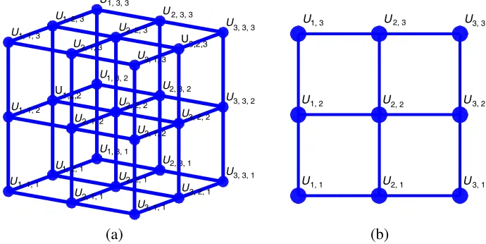
U(x, y, z) must vary linearly as a function of position. To numerically solve Eq. (2) using the finite-difference method, the functionU(x, y, z) is stored at discrete points on a grid as illustrated in Figure 1. This figure shows a small 3D grid and an analogous 2D grid which stores the discretized function Ui,j.
U U U U U U3,2,3 U U U U U U U U U U U U U U U U U 1,2,2 U U U U U U U U U U U U U (a) (b)
1, 3 2, 3 3, 3
1, 2 2, 2 3, 2
1, 1 2, 1 3, 1
1, 3, 3
2, 3, 3
3, 3, 3
3, 3, 2
3, 3, 1 1, 2, 3
1, 1, 3
1, 1, 2
1, 1, 1
2, 1, 3
2, 1, 2
2, 1, 1 1, 2, 1
1, 3, 1
3, 1, 1 3, 2, 1 2, 2, 1
2, 2, 2 2, 3, 2
3, 2, 2
3, 1, 2
2, 3, 1 1, 3, 2
3, 1, 3 2, 2, 3
Figure 1. (a) Three-dimensional grid forU(x, y, z). (b) Two-dimensional grid forU(x, y).
This allows the second-order derivatives in Eq. (2) to be approximated with central finite-differences as follows.
Ui+1,j,k−2Ui,j,k+Ui−1,j,k
Δx2 +
Ui,j+1,k−2Ui,j,k+Ui,j−1,k
Δy2 +
Ui,j,k+1−2Ui,j,k+Ui,j,k−1
Δz2 ≈0 (3)
Equation (3) can be interpreted as enforcing Laplace’s equation on the discrete function Ui,j,k at point (i, j, k). To enforce Laplace’s equations across the entire grid, Eq. (3) is written once for every point on the grid. This large set of equations can be written in matrix form as
Lu=0 (4)
In Eq. (4), the termucontains all of the unknown values ofUi,j,kthroughout the entire grid reshaped into a one-dimensional column vector. The square matrix L operates onu to calculate its scalar Laplacian
2.2. Matrix Operator Approach
Given a discrete function Ui,j,k stored in a column vector u, it is always possible to construct a square matrixL that performs any linear operation onu including derivatives [10, 11], discrete Fourier transforms [12, 13], convolutions [13], and more. Linearity makes it possible to breakdown complex linear operations into combinations of simpler linear operations. From Eq. (2), it is possible to express the Laplacian operationL as the sum of three derivative operations D2x,D2y, and D2z to get Eq. (5).
L=D2x+D2y+D2z (5)
The termsD2x,D2y, and D2z are square banded matrices the same size as L that calculate second-order derivatives of the functionuacross the entire grid. These are simpler to construct thanLand easier to verify if they are correct, so it is often advantageous to construct these first and then calculate L from them using Eq. (5).
As an example, the matrix Laplacian L will be constructed for the two-dimensional 3×3 point grid shown in Figure 1. First, suppose we wish to calculate the second-order derivative of Ui,j in thex direction. The finite-difference approximation for this can be written as
∂2U i,j
∂x2 ≈
Ui+1,j−2Ui,j+Ui−1,j
Δx2 . (6)
This equation is written once for every point on the grid and the large set of equations is collected into a single matrix equation. The matrix equation is expressed as a square matrix operating on the column vectoru. The square matrix derived from this process is the matrix derivative operatorD2xas expressed in Eq. (7).
D2xu= 1 Δx2
⎡ ⎢ ⎢ ⎢ ⎢ ⎢ ⎢ ⎢ ⎢ ⎢ ⎢ ⎣
U2,1−2U1,1
U3,1−2U2,1+U1,1
−2U3,1+U2,1
U2,2−2U1,2
U3,2−2U2,2+U1,2
−2U3,2+U2,2
U2,3−2U1,3
U3,3−2U2,3+U1,3
−2U3,3+U2,3
⎤ ⎥ ⎥ ⎥ ⎥ ⎥ ⎥ ⎥ ⎥ ⎥ ⎥ ⎦ = 1 Δx2
⎡ ⎢ ⎢ ⎢ ⎢ ⎢ ⎢ ⎢ ⎢ ⎢ ⎢ ⎣
−2 1 1 −2 1
1 −2 0 0 −2 1
1 −2 1 1 −2 0
0 −2 1 1 −2 1
1 −2
⎤ ⎥ ⎥ ⎥ ⎥ ⎥ ⎥ ⎥ ⎥ ⎥ ⎥ ⎦ ⎡ ⎢ ⎢ ⎢ ⎢ ⎢ ⎢ ⎢ ⎢ ⎢ ⎢ ⎣
U1,1
U2,1
U3,1
U1,2
U2,2
U3,2
U1,3
U2,3
U3,3
⎤ ⎥ ⎥ ⎥ ⎥ ⎥ ⎥ ⎥ ⎥ ⎥ ⎥ ⎦ . (7) A problem arises when writing Eq. (6) at both the left and right sides of the grid where values of
Ui,j are needed from outside of the grid. The manner in which this is handled is called a numerical boundary condition [14, 15]. To arrive at Eq. (7), it was assumed that all values of Ui,j were zero outside of the grid. This is called the Dirichlet boundary condition [16, 17]. Second, the finite-difference approximation for the second-order derivative of Ui,j in they direction can be written as
∂2U i,j
∂y2 ≈
Ui,j+1−2Ui,j+Ui,j−1
Δy2 . (8)
This equation is also written once for every point on the grid and the large set of equations is collected into a single matrix equation expressed as a square matrix operating on the column vector u. The square matrix derived from this process is the matrix derivative operator D2y as expressed in Eq. (9).
D2yu= 1 Δy2
⎡ ⎢ ⎢ ⎢ ⎢ ⎢ ⎢ ⎢ ⎢ ⎢ ⎢ ⎣
U1,2−2U1,1
U2,2−2U2,1
U3,2−2U3,1
U1,3−2U1,2+U1,1
U2,3−2U2,2+U2,1
U3,3−2U3,2+U3,1
−2U1,3+U1,2
−2U2,3+U2,2
−2U3,3+U3,2
⎤ ⎥ ⎥ ⎥ ⎥ ⎥ ⎥ ⎥ ⎥ ⎥ ⎥ ⎦ = 1 Δy2
⎡ ⎢ ⎢ ⎢ ⎢ ⎢ ⎢ ⎢ ⎢ ⎢ ⎢ ⎣
−2 1
−2 1
−2 1
1 −2 1
1 −2 1
1 −2 1
1 −2
1 −2
1 −2
⎤ ⎥ ⎥ ⎥ ⎥ ⎥ ⎥ ⎥ ⎥ ⎥ ⎥ ⎦ ⎡ ⎢ ⎢ ⎢ ⎢ ⎢ ⎢ ⎢ ⎢ ⎢ ⎢ ⎣
U1,1
U2,1
U3,1
U1,2
U2,2
U3,2
U1,3
U2,3
U3,3
Dirichlet boundary conditions were used again here at the top and bottom boundaries of the grid. Third, the Laplacian matrix L for two dimensions is calculated by summing the above two derivative matrices.
L=D2x+D2y (10)
2.3. Enforcing Physical Boundary Conditions
At this point, our matrix equation has the form Lu=0. If this was solved foruonly a trivial solution would be obtained. The matrix equation can be written in a solvable form Lu=b when the physical boundary conditions are incorporated. To do this, at least some values of Ui,j on the grid must be known. Each known point is incorporated into the matrix equation by: (1) replacing the entire row in the matrix equation corresponding to that point with all 0’s, (2) placing a 1 in the diagonal position in
L, and (3) placing the known value of Ui,j into that same row of b.
All of this can be accomplished in a more straightforward manner as follows. First, a force matrixF
is constructed. This is a diagonal matrix with 1’s placed in the positions along diagonal that correspond to points with known vales of Ui,j. Second, a force function UF,i,j is constructed that contains all of the known values placed at the correct points on the grid. The force function is reshaped into a one-dimensional column vector uF called the force vector. It may seem tedious or more complicated to construct these functions and matrices, but they need to be constructed anyway to describe arbitrary devices. Given the force matrix F and the force vector uF, the matrix equation incorporating these physical boundary conditions is
Lu=b (11)
where
L = F+ (I−F)L (12)
b = FuF (13)
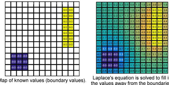
The termI is the identity matrix. A solution to Eq. (11) is calculated asu=L−1b. An example for a 13×13 point grid is provided in Figure 2. At left is the empty grid highlighting the known points, or physical boundary conditions. At right is the functionUi,j after solving Laplace’s equations with these boundary conditions. From this, we see that Laplace’s equation provides a way to fill in all the other values of a function so that they vary linearly in the space between the physical boundary conditions.
Figure 2. Two-dimensional grid to illustrate solution of Laplace’s equation.
2.4. Enclosed Problems
(a) (b)
Figure 3. (a) Physical boundary conditions enclose a portion of the grid. (b) Solution to Laplace’s equations obtained only in the enclosed portion of the grid.
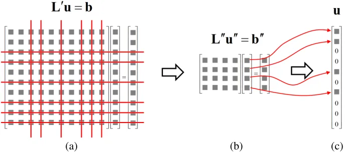
(a) (b) (c)
Figure 4. (a) Matrix equation Lu = b for entire grid. (b) Reduced Laplace’s equation. (c) Repopulated full size column vector u.
efficient to only solve Laplace’s equation within the enclosed region and not outside. This situation arises when designing devices by TO since the transform is typically contained within the volume of the device. A simple case of this concept is illustrated in Figure 3 where an arbitrary region of the grid is enclosed by the physical boundary conditions. The solution to Laplace’s equation fills in the values inside the enclosed region, but no solution is obtained outside of the enclosed region.
The procedure to reduce Laplace’s equation is simple. All of the points on the grid are identified where a solution to Laplace’s equation is needed. The rows and columns corresponding to all other points are dropped from the matrix equation. The reduced matrix equation can be written as
Lu=b. (14)
2.5. Numerical Grid Generation
Numerical grid generation is used in fields such as oceanography [18], computational fluid dynamics [19– 21], and conformal mapping in electromagnetics [6]. The approach allows complex geometries to be handled by mapping an arbitrary grid to a Cartesian grid. The most common approach is based on solving Laplace’s equation [20, 22] for the transformed coordinates because it generates coordinates that vary linearly. Given the boundary conditions for an arbitrary coordinate transformation from{x, y, z} to{x, y, z}, Laplace’s equation can be used to solve for the transformed coordinates using the following equations.
∇2x =
∂2
∂2x +
∂2
∂2y +
∂2
∂2z
x = 0 (15)
∇2y =
∂2
∂2x +
∂2
∂2y +
∂2
∂2z
y = 0 (16)
∇2z =
∂2
∂2x +
∂2
∂2y +
∂2
∂2z
z = 0 (17)
Occasionally, the backward coordinate transformation is advantageous. Examples of such cases will be discussed later. In the case where the backward coordinate transformation is favored, Laplace’s equation can be solved for the backward transformation according to
∇2x =
∂2
∂2x +
∂2
∂2y +
∂2
∂2z
x= 0 (18)
∇2y =
∂2
∂2x +
∂2
∂2y +
∂2
∂2z
y= 0 (19)
∇2z =
∂2
∂2x +
∂2
∂2y +
∂2
∂2z
z= 0. (20)
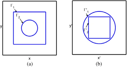
The solutions of Eqs. (15)–(20) yields only the trivial solution until the boundary conditions are enforced. Consider the two arbitrary boundaries shown in Figure 5. The boundary conditions along the outer boundary Γ1 and the inner boundary Γ2 are given by
Ux, y|
Γ1(x,y) = U(x, y)|Γ1(x,y) (21)
Ux, y|
Γ2(x,y) = U(x, y)|Γ2(x,y) (22)
The force matrix and force vector are used to incorporate the boundary conditions into Eqs. (21) and (22). The force matrix F contains 1’s along the diagonal in the positions that correspond to the boundaries of the device which have known coordinate values. The force vector uF is a column vector
(a) (b)
containing the values ofU(x, y) at the boundaries. Given these two terms, the matrix equation can be put into a solvable form consistent with Eqs. (11)–(13). The matrix equation is further reduced to the form of Eq. (14) by dropping all rows and columns for points outside of the enclosed region being solved. This final equation can be solved using any standard algorithm such as an optimized LU decomposition algorithm for sparse linear systems [23] or an iterative solver such as the conjugate gradient method [24]. As the boundary problem shown in Figure 5 is only defined on the x-y plane, the z coordinate is not necessary and can be omitted from the Laplace’s equations leaving just the following two equations to solve.
∇2x =
∂2
∂x2 +
∂2
∂y2
x= 0 (23)
∇2y =
∂2
∂x2 +
∂2
∂y2
y = 0 (24)
Equations (23) and (24) are approximated with finite-differences and put into matrix form. The boundary conditions are applied using the force matrixFand two force vectorux,F anduy,F. The force vectorsux,F anduy,F contain thexcoordinates and ycoordinates respectively defined by the boundary conditions. The matrix equation is then reduced by eliminating the rows and columns corresponding to points outside of the outer boundary. This gives two matrix equations to be solved within the region being transformed.
Lx = bx (25)
Ly = by (26)
These are solved according to
x = A−1bx (27)
y = A−1by. (28)
Figure 6 displays the result of solving the boundary value problem for the coordinate transformation from {x, y} → {x, y}.
(a) (b)
Figure 6. Coordinate transformation boundary value problem shown in Figure 5. (a) Original Cartesian coordinate system within the transformation boundaries. (b) Transformed coordinate system determined using the boundaries shown in Figure 5 and defined in Eqs. (21) and (22).
3. CALCULATING THE PERMITTIVITY AND PERMEABILITY FUNCTIONS
the grid [1].
ε
r = Λ[εr]Λ T
detΛ (29)
μr = Λ[μr]Λ
detΛ (30)
These equations come from a forward coordinate transform so they involve the Jacobian matrix Λ
defined by
Λ=
Λ
xx Λxy Λxz
Λyx Λyy Λyz Λzx Λzy Λzz
= ⎡ ⎢ ⎢ ⎢ ⎢ ⎢ ⎢ ⎣ ∂x ∂x ∂x ∂y ∂x ∂z ∂y ∂x ∂y ∂y ∂y ∂z ∂z ∂x ∂z ∂y ∂z ∂z ⎤ ⎥ ⎥ ⎥ ⎥ ⎥ ⎥ ⎦ (31)
The elements of the Jacobian matrix can be computed numerically using finite-differences [5, 25] and stored as arrays as follows.
Λxx(i, j, k) = ∂x
∂x ∼= x
i+1,j,k−xi−1,j,k
2Δx (32)
Λxy(i, j, k) = ∂x
∂y ∼= x
i,j+1,k−xi,j−1,k
2Δy (33)
Λxz(i, j, k) = ∂x
∂z ∼= x
i,j,k+1−xi,j,k−1
2Δz (34)
Λyx(i, j, k) = ∂y
∂x ∼= y
i+1,j,k−yi−1,j,k
2Δx (35)
Λyy(i, j, k) = ∂y
∂y ∼= y
i,j+1,k−yi,j −1,k
2Δy (36)
Λyz(i, j, k) = ∂y
∂z ∼= y
i,j,k+1−yi,j,k−1
2Δz (37)
Λzx(i, j, k) = ∂z
∂x ∼= z
i+1,j,k−zi−1,j,k
2Δx (38)
Λzy(i, j, k) = ∂z
∂y ∼= z
i,j+1,k−zi,j −1,k
2Δy (39)
Λzz(i, j, k) = ∂z
∂z ∼= z
i,j,k+1−zi,j,k −1
2Δz (40)
For two-dimensional devices like this that are uniform in the z-direction, it is only necessary to calculate four elements of the Jacobian,Λxx,Λxy,Λyx, andΛyy. The elementsΛxz,Λyz,Λzx, andΛzy
are arrays of all zeros and Λzz is an array of all ones.
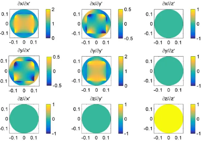
Iterating through the grid point-by-point, the Jacobian matrix at each grid position is assembled according to Eq. (31) with the derivatives evaluated at each point. Depending on how the coordinate transformations were determined, it is sometimes necessary to calculate the Jacobian for the backward coordinate transformation according to
Λ =
⎡ ⎣
Λxx Λxy Λxz Λyx Λyy Λyz Λzx Λzy Λzz
⎤ ⎦= ⎡ ⎢ ⎢ ⎢ ⎢ ⎢ ⎢ ⎣ ∂x ∂x ∂x ∂y ∂x ∂z ∂y
∂x ∂y∂y ∂z∂y
Figure 7. Elements composing the Jacobian matrix for the coordinate transformation shown in Figure 6.
The calculated derivatives are each stored in an array the same size as the grid as shown in Figure 7. The forward Jacobian matrix can be found from the backward Jacobian matrix by calculating the inverse [26–28]. The permittivity tensor is calculated at the point i,j,kwithin the grid using Eq. (29) with the Jacobian matrix appropriate to the coordinate transformation. The permittivity tensor can be written where each element is stored as an array.
εr(i, j, k)=
⎡ ⎣ ε
xx(i, j, k) εxy(i, j, k) εxz(i, j, k)
ε
yx(i, j, k) εyy(i, j, k) εyz(i, j, k)
ε
zx(i, j, k) εzy(i, j, k) εzz(i, j, k)
⎤
⎦ (42)
Likewise, the permeability tensor can be written as
μr(i, j, k)=
⎡ ⎣ μ
xx(i, j, k) μxy(i, j, k) μxz(i, j, k)
μ
yx(i, j, k) μyy(i, j, k) μyz(i, j, k)
μ
zx(i, j, k) μzy(i, j, k) μzz(i, j, k)
⎤
⎦ (43)
4. IMPROVED ANISOTROPIC FINITE-DIFFERENCE FREQUENCY-DOMAIN
Electromagnetic simulation of TO devices can be performed using the AFDFD method, which is described in detail in Ref. [5]. The key matrix equation to be solved in the conventional AFDFD
is
Ch[μr]−1Ce−[εr]
e=0. (44)
where Ch and Ce are the curl operator matrices for the magnetic field intensity and electric field intensity respectively, [μr] is the permeability tensor, and [εr] is the permittivity tensor as described in detail in Ref. [5]. When simulating devices with magnetically anisotropic materials, the matrix division involving the permeability tensor is very slow and numerically inefficient. To mitigate this, Eq. (44) is instead solved using the impermeability matrix [ψ]
Ch[ψ]Ce−[εr]
e = 0 (45)
To calculate [ψ] most efficiently, the elements are calculated when they are still functions stored in arrays and not yet diagonal matrices. In this context, we have
[ψ(i, j, k)] =
⎡
⎣ ψψxxyx((i, j, ki, j, k)) ψψxyyy((i, j, ki, j, k)) ψψxzyz((i, j, ki, j, k))
ψzx(i, j, k) ψzy(i, j, k) ψzz(i, j, k)
⎤ ⎦=
⎡
⎣ μμxxyx((i, j, ki, j, k)) μμxyyy((i, j, ki, j, k)) μμyzxz((i, j, ki, j, k))
μzx(i, j, k) μzy(i, j, k) μzz(i, j, k)
⎤ ⎦
−1
.
(47) The elements of [ψ(i, j, k)] are derived from the tensor [μr(i, j, k)] by calculating the matrix inverse symbolically.
[ψ(i, j, k)] =
μ
yyμzz −μyzμzy μxzμzy−μxyμzz μxyμyz−μxzμyy
μyzμzx−μyxμzz μxxμzz−μxzμzx μxzμyx−μxxμyz
μyxμzy−μyyμzx μxyμzx−μxxμzy μxxμyy−μxyμyx
μxxμyyμzz−μxxμyzμzy−μxzμyyμzx−μxyμyxμzz+μxyμyzμzx+μxzμyxμzy (48) For brevity, the dependence on the array indices i, j, and k have been dropped from these equations. All of these calculations are performed point-by-point on arrays instead of with matrices. After the elements of [ψ(i, j, k)] are calculated, they are reshaped into diagonal matrices and assembled into the overall impermeability matrix as follows.
[ψ] =
ψ
xx ψxy ψxz ψyx ψyy ψyz ψzx ψzy ψzz
(49)
whereψmn= diag{ψmn(i, j, k)}.
Using the impermeability tensor rather than the permeability tensor to solve the wave equation in Eq. (45) decreased the time required to solve a two dimensional AFDFD simulation for a flat TO lens on a 90×77 cell grid from 727.18 seconds to 8.33 seconds. Also the amount of memory required to solve AFDFD using the impermeability tensor was drastically reduced compared to the conventional AFDFD algorithm using the permeability tensor. The simulation with the impermeability tensor required 105.7 MB to be allocated whereas the simulation with the permeability tensor required 6.962 GB to be allocated.
5. BENCHMARK AND EXAMPLES
5.1. Cylindrical Electromagnetic Cloak
To benchmark our approach, we duplicated the famous cylindrical electromagnetic cloak presented in Ref. [2]. This was based on the closed form coordinate transformation given by
r=R
1+rR2R−R1 2
θ=θ
z =z
(50)
where the cloak has an inner radius R1 and outer radius R2. Figure 8 shows the outlines of the boundaries of the coordinate transformation given by Eq. (50).
In order to calculate the coordinate transformation numerically, the following boundary conditions were applied
Γ2x, y = Γ2(x, y) (51)
Γ1x, y = 0 (52)
Figure 8. Coordinate transformation boundary conditions for a cylindrical cloak.
Figure 9. AFDFD simulation of cylindrical electromagnetic cloak.
Figure 10. Permittivity tensor for cylindrical electromagnetic cloak. The permeability tensor is identical for a cloak based in free space. All tensor components which are not visualized are equal to one for the elements along the diagonal and zeros for the off-diagonal elements. The values determined for this cloak are based on a grid resolution ofλ0/120. As the grid resolution is made smaller, the values of the materials required would approach infinity or zero due the cloaked region being a singularity.
The device was simulated using the improved AFDFD. Dirichlet boundary conditions were used for the y-axis boundaries while a uniaxial perfectly matched layer (UPML) was used for the x-axis boundaries. The result is shown in Figure 9.
5.2. Flat Lens
Figure 11 shows the boundary conditions necessary to design a flat lens using TO as described in Ref. [29]. By solving Laplace’s equation for the boundaries
Γ1 →Γ1
Γ2 →Γ2
Γ3 →Γ3 Γ4 →Γ4
(a) (b)
Figure 11. Coordinate transformation for transformation optics bend. (a) is the original coordinate space while that (b) is the transformed space.
Figure 12. AFDFD simulation of flat TO lens.
Figure 13. Permittivity tensors for flat transformation optics lens. The permeability tensor is identical for a bend based in free space. All tensor components which are not visualized are zero throughout the grid. The material values for this lens are for a grid resolution of λ0/120.
the coordinate transformation was computed numerically.
With the coordinates in the new system known, the Jacobian matrix was calculated using Eq. (31) and the material tensors determined using Eqs. (29) and (30). The resulting permittivity is shown in Figure 13. The permeability is identical to the permittivity in this situation because the original space is vacuum.
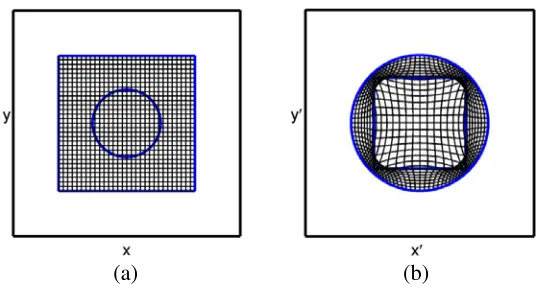
5.3. Arbitrary Cloak
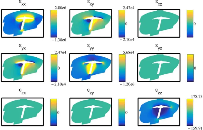
This section will demonstrate the method implemented above with the arbitrary metamaterial cloak shown in Figure 14. The pickaxe shape bounded by Γ1 is being cloaked by the region bounded by Γ2. In order to cloak the object, a coordinate system in which the axes wrap around the object without penetrating the object itself must be implemented within the region between the two boundaries. In order to avoid singular Jacobian matrices in the cloaked region, the backward coordinate transformation was implemented rather than the forward transformation. The boundary conditions, which were derived from those described in Ref. [3], are given as follows.
Γ2x, y = Γ2(x, y) (54)
Γ1x, y = 0 (55)
Following the procedure described in the previous sections of this paper the material tensors were calculated. The resulting permittivity tensor is shown in Figure 16 with the permeability tensor being the same.
Figure 14. Outline of arbitrary electromagnetic cloak and object to be cloaked.
Figure 15. AFDFD simulation of arbitrary electromagnetic cloak.
Using AFDFD, the TO cloak was simulated for a TM polarized wave as shown in Figure 15. The material tensors for the cloak were placed between a UPML on the x-axis boundaries and Dirichlet boundary conditions on the y-axis boundaries. As can be seen, very little power is scattered and the phase of the wave is very well preserved.
5.4. Transformation Optics Bend
Creating a bend using numerical TO involves solving Laplace’s equation for the boundary value problem shown in Figure 17. Rather than transform from {x, y} to {x, y}, the backward transformation was chosen because mapping the arbitrarily distorted boundaries shown on the right in Figure 17 to the boundaries of the original system could be done with simple analytical expressions. Solving Laplace’s
(a) (b)
Figure 17. Coordinate transformation for transformation optics bend. (a) is the original coordinate space while that (b) is the transformed space.
Figure 18. AFDFD simulation of TO electro-magnetic bend.
equation with the boundary values
Γ1 →Γ1 Γ2 →Γ2
Γ3 →Γ3
Γ4 →Γ4
(56)
provides the coordinates of the backward coordinate transformation.
Using the procedure described above, the material tensors were calculated as shown in Figure 19 and placed in a grid surrounded by a UPML. This was simulated using AFDFD and the result is shown in Figure 18.
6. CONCLUSIONS
A simple technique for generating and simulating TO devices with arbitrary geometry was described in this article. Laplace’s equation was used to generate the coordinates of the spatial transforms. The method described uses a finite-difference approach so it is simple and straightforward to implement. Other approaches in the literature used commercial software such as COMSOL, making it difficult or impossible to import and export complex data. The technique described in this paper can be implemented independent of a commercial solver and in virtually any programming environment. This allows much greater flexibility in manipulating the data and importing the generated materials into custom electromagnetic solvers such as finite-difference time-domain, finite-difference frequency-domain, beam propagation method, and more. Further, an improvement to the standard AFDFD method was outlined that greatly improves the speed and efficiency for simulating TO devices. The new approach utilized the impermeability tensor instead of the permeability tensor in the matrix wave equation.
Several examples were presented to benchmark the approach and demonstrate its versatility. The devices included the classical cylindrical cloak, an arbitrarily shaped cloak, a flat lens, and an arbitrarily shaped bend. Devices with arbitrary shapes were verified through simulation using the improved AFDFD. The simulation results showed excellent performance of the devices.
REFERENCES
1. Pendry, J. B., D. Schurig, and D. R. Smith, “Controlling electromagnetic fields,”Science, Vol. 312, 1780–1782, 2006.
2. Schurig, D., J. Mock, B. Justice, S. A. Cummer, J. B. Pendry, A. Starr, et al., “Metamaterial electromagnetic cloak at microwave frequencies,” Science, Vol. 314, 977–980, 2006.
3. Hu, J., X. Zhou, and G. Hu, “Design method for electromagnetic cloak with arbitrary shapes based on Laplace’s equation,”Optics Express, Vol. 17, 1308–1320, 2009.
4. Chang, Z., X. Zhou, J. Hu, and G. Hu, “Design method for quasi-isotropic transformation materials based on inverse Laplace’s equation with sliding boundaries,”Optics Express, Vol. 18, 6089–6096, 2010.
5. Rumpf, R. C., C. R. Garcia, E. A. Berry, and J. H. Barton, “Finite-difference frequency-domain algorithm for modeling electromagnetic scattering from general anisotropic objects,” Progress In Electromagnetics Research B, Vol. 61, 55–67, 2014.
6. Landy, N. I. and W. J. Padilla, “Guiding light with conformal transformations,” Optics Express, Vol. 17, 14872–14879, 2009.
7. Ma, J.-J., X.-Y. Cao, K.-M. Yu, and T. Liu, “Determination the material parameters for arbitrary cloak based on Poisson’s equation,” Progress In Electromagnetics Research M, Vol. 9, 177–184, 2009.
9. Rumpf, R. C. and J. Pazos, “Synthesis of spatially variant lattices,” Optics Express, Vol. 20, 15263–15274, 2012.
10. Smith, G. D., Numerical Solution of Partial Differential Equations: Finite Difference Methods, Oxford University Press, 1985.
11. LeVeque, R. J., “Finite difference methods for differential equations,” Draft Version for Use in AMath, Vol. 585, 1998.
12. Golub, G. H. and C. F. van Loan,Matrix Computations, Vol. 3, JHU Press, 2012.
13. Johnson, H. and C. S. Burrus, “On the structure of efficient DFT algorithms,”IEEE Transactions on Acoustics, Speech and Signal Processing, Vol. 33, 248–254, 1985.
14. Iserles, A., A First Course in the Numerical Analysis of Differential Equations, Cambridge University Press, 2009.
15. Chapra, S. C. and R. P. Canale,Numerical Methods for Engineers, Vol. 2, McGraw-Hill, 2012. 16. Arfken, G. and H. Weber,Mathematical Methods for Physicists, 6th Edition, Academic, New York,
2005.
17. Morgan, M. A., Finite Element and Finite Difference Methods in Electromagnetic Scattering, Elsevier, 2013.
18. Luong, P., “A mathematical coastal ocean circulation system with breaking waves and numerical grid generation,”Applied Mathematical Modelling, Vol. 21, 633–641, 1997.
19. Eiseman, P. R., “Grid generation for fluid mechanics computations,” Annual Review of Fluid Mechanics, Vol. 17, 487–522, 1985.
20. Thompson, J. F., Z. U. Warsi, and C. W. Mastin, Numerical Grid Generation: Foundations and Applications, Vol. 45, North-holland Amsterdam, 1985.
21. Sanmiguel-Rojas, E., J. Ortega-Casanova, C. del Pino, and R. Fernandez-Feria, “A Cartesian grid finite-difference method for 2D incompressible viscous flows in irregular geometries,” Journal of Computational Physics, Vol. 204, 302–318, 2005.
22. Akcelik, V., B. Jaramaz, and O. Ghattas, “Nearly orthogonal two-dimensional grid generation with aspect ratio control,”Journal of Computational Physics, Vol. 171, 805–821, 2001.
23. Davis, T. A., “Algorithm 832: UMFPACK V4.3 — An unsymmetric-pattern multifrontal method,”
ACM Transactions on Mathematical Software (TOMS), Vol. 30, 196–199, 2004.
24. Paige, C. C. and M. A. Saunders, “Solution of sparse indefinite systems of linear equations,”SIAM Journal on Numerical Analysis, Vol. 12, 617–629, 1975.
25. Rumpf, R. C., “Simple implementation of arbitrarily shaped total-field/scattered-field regions in finite-difference frequency-domain,” Progress In Electromagnetics Research B, Vol. 36, 221–248, 2012.
26. Schutz, B.,A First Course in General Relativity, Cambridge University Press, 2009.
27. Hobson, M. P., G. P. Efstathiou, and A. N. Lasenby, General Relativity: An Introduction for Physicists, Cambridge University Press, 2006.
28. Liseikin, V., “Coordinate transformations,” Grid Generation Methods, 31–66, Springer, Netherlands, 2010.