A Fast Motion Parameters Estimation Method Based
on Cross-Correlation of Adjacent Echoes for
Wideband LFM Radars
Yixiong Zhang1,*,Rujia Hong1,†,Cheng-Fu Yang2,*, Yunjian Zhang1,†,Zhenmiao Deng1,†,and Sheng Jin3,†
1 School of Information Science and Engineering, Xiamen University, Xiamen, China; [email protected] (R.H.); [email protected] (Y.Z.); [email protected] (Z.D.)
2 Department of Chemical and Materials Engineering, National University of Kaohsiung, Kaohsiung, Taiwan 3 Beijing Institute of Tracking and Telecommunications Technology, Beijing, China; [email protected] * Correspondence: [email protected] (Y.Z.); [email protected] (C.-F.Y.); Tel.:+ 86-592-2965385 (Y.Z.);
+00886-7591-9283 (C.-F.Y.).
† These authors contributed equally to this work.
Abstract: In wideband radar systems, the performance of motion parameters estimation can significantly affect the performance of object detection and the quality of inverse synthetic aperture radar (ISAR) imaging. Although the traditional motion parameters estimation methods can reduce the range migration (RM) and Doppler frequency migration (DFM) effects in ISAR imaging, the computational complexity is high. In this paper, we propose a new fast non-searching motion parameters estimation method based on cross-correlation of adjacent echoes (CCAE) for wideband LFM signals. A cross-correlation operation is carried out for two adjacent echo signals, then the motion parameters can be calculated by estimating the frequency of the correlation result. The proposed CCAE method can be applied directly to the stretching system, which is commonly adopted in wideband radar systems. Simulational results demonstrate that the new method can achieve better estimation performances, with much lower computational cost, compared with existing methods. The experimental results on real radar data sets are also evaluated to verify the effectiveness and superiority of the proposed method compared to the state-of-the-art existing methods.
Keywords:motion parameters estimation, wideband LFM radar, cross-correlation.
1. Introduction
The wideband linear frequency modulation (LFM) signal is widely used in modern wideband radar systems. Compared with the narrow-band LFM signal, it can achieve much better quality in inverse synthetic aperture radar (ISAR) imaging, due to the higher range resolution. However, the motions of target often cause range migration (RM) and Doppler frequency migration (DFM) effects in the received signals, which will degrade the imaging quality. Therefore, the object’s motion parameters should be estimated and compensated before imaging. Besides, the accuracy of motion parameters estimation also affects the performance of target tracking and identification. Thus, high precision motion parameters estimation is necessary and attracts much more attention in modern wideband radar systems [1–8].
For wideband radars, the estimation methods of motion parameters can be divided into two types: searching methods and non-searching methods. Many of the traditional range alignment methods [8–14] in ISAR imaging are of searching methods, such as spatial domain realignment [8], adaptive joint time-frequency technique [9], minimum entropy method [14]. Spatial domain realignment [8] defines a correlation function between two envelops of echo signals with delays. The amount of envelope shift is determined by searching the delay to obtain the maximum of the correlation function. In [9], the radar echo signal is projected to a set of basis functions, which are constructed with different parameters. A searching procedure is conducted to maximize the projection value, and then the
motion parameters estimated. The minimum entropy method introduces a 1-D entropy function to determine the degree of alignment between radar echoes [14]. As the delay, which minimizes the entropy, is searched with the step determined by the bandwidth of the transmitted signal, the accuracy of the estimated parameters is limited by the delay step. To perform high precision motion parameters estimation, the Radon Fourier transform (RFT) method is proposed for multipulse energy accumulation [5,15,16]. The RFT method is a multidimensional searching method and achieves a good performance of motion parameters estimation because of long coherent integration time. A common drawback of these searching methods is that their computation is highly complex, when they are applied in the wideband radar systems.
In the non-searching methods, the keystone transform (KT) is able to eliminate the RM effect based on long time coherent integration technology [17–19]. But the DFM induced by acceleration cannot be removed by KT. In [20], a non-searching ISAR range alignment method based on minimizing the entropy of the average range profile (ARP) is proposed. An iterative procedure is utilized to estimate the delays of envelops, of which the precision is determined by the range resolution. Meanwhile, an interpolation is employed on the envelops to improve the estimation precision. However, the iterative procedure and the interpolation operation significantly increase the computational complexity. Moreover, the phase information is not used for estimation in [20]. In [21], a novel estimation algorithm of motion parameters is proposed for ISAR imaging, based on KT and the adjacent cross-correlation function (ACCF). Then, a fast non-searching method based on ACCF is proposed for target motion estimation, target detection and ISAR imaging [22–26]. There are two differences between the two methods in [21] and in [22–26]. The first one is that the KT is not utilized in [22–26], and the other one is that the choice of the scaling factors is improved in [26], thus better performance is obtained under low SNR conditions. Compared with the RFT method, the ACCF method [22,23] can achieve similar performance with much lower computational cost. However, it can be applied only to the uncompressed received (UR) signal, whose bandwidth is equal to that of the transmitted wideband LFM signal. In order to reduce the processing bandwidth and the sampling rate of the analog-to-digital converter, the stretching processing is commonly used in most of the wideband LFM radars, and therefore, the ACCF method cannot be applied in these radar systems.
In this paper, a novel and fast estimation method based on cross-correlation of adjacent echoes (CCAE) is proposed. Specifically, the cross-correlation operation is performed on two adjacent echo signals, then the motion parameters are calculated by estimating the frequency of the correlation result. The proposed new method is a non-searching method and can be directly applied to the stretched signals. Since the SNR of the stretched signal is higher than that of the UR signal, better root-mean-square errors (RMSE) performance can be achieved by applying the CCAE method to the stretched signals. When estimating the velocity using two echo signals, the FFT operation is needed only once in the CCAE method. Thus, the computational complexity of the proposed CCAE method is much lower than that of the existing methods. Numerical simulations demonstrate that the proposed CCAE method can be applied in real wideband LFM radars.
The rest of this paper is organized as follows. In Section2, the model of the stretched signal is presented. In Section3, the proposed fast non-searching CCAE method is presented first, and then the root mean square error (RMSE) of the proposed CCAE method derived in closed form. In Section 4, the details of the experiments conducted on simulation and real data are presented. Finally, we conclude this paper in Section5.
2. Signal Model
Range window Incident
Wave front
Range
In
te
n
si
ty
Range Profile radar scatterers
Figure 1.Target’s range profile of wideband radar
Table 1.Notations.
Notation Type Meaning
ur Subscript The received signal is uncompressed.
st Subscript The signal is stretched.
ac Subscript The signal is obtained by multiplying a echo signal with the conjugate of another echo signal. se Subscript The signal is the multiplication result of the different echo signal from the same scatterers. cr Subscript The signal is the multiplication result of the different echo signal from the different scatterers.
str(t) Signal The transmitted signal.
sLO(t) Signal The local reference signal.
sur(t,tm) Signal The uncompressed received signal.
sst(t,tm) Signal The stretched signal.
Rp(tm) Signal The distance from radar to thepth scatterer.
The transmitted signal of the wideband LFM radar can be modeled as
str(t) =rect
t T
ejπγt2ej2πfct, (1)
where rect(u) = (
1,|u| ≤1/2
0, otherwise denotes the rectangle pulse shape,tthe fast time,Tthe pulse width, andfcthe radar center frequency.γ=B/Tis the chirp rate of the LFM signal, whereBis the swept bandwidth of the LFM signal.
The UR signal of the wideband LFM radar can be represented as
sur(t,tm) =
P−1
∑
p=0
rect
t−
τp(tm)
T
×Apej2πfc(t−τp(tm)) ×ejγπ(t−τp(tm))2+ω
0(t,tm)
=sur,s(t,tm) +ω0(t,tm), (2)
wherePdenotes the number of scatterers,Apthe scattering coefficient of thepth scatterer, andτp(tm)
the time delay from the radar to thepth scatterer.tm =mTpr is the slow time, wheremis the pulse
number, andTpris the pulse repetition interval (PRI).sur,s(t,tm)denotes the signal term ofsur(t,tm), ω0(t,tm)is the Gaussian noise with mean zero and varianceσ2. The time delay can be expressed as
τp(tm) =2
Rp(tm)
whereRp(tm)is the distance from radar to thepth scatterer at slow timetm. Due to the wide bandwidth
of the signal, the data size of the uncompressed signal is considerably large, which leads to a high computational complexity. Therefore, in wideband radar systems, stretching operation is often used to reduce the data size.
The local reference signal for stretching operation can be written as
sLO(t) =rect
t ˆ T
e−j(2πfct+πγt2), (4)
where ˆT is the duration of the reference signal, which is usually slightly larger than the width of the transmitted pulse, so that it covers the received signal. The stretched signal is obtained by multiplication
sst(t,tm) =sur(t,tm)·sLO(t) =
P−1
∑
p=0
rect
t−
τp(tm)
T
Ape−j2πγτp(tm)t
×ejπγτ2p(tm)e−j2πfcτp(tm)+ω
1(t,tm)
=sst,s(t,tm) +ω1(t,tm), (5)
wheresst,s(t,tm)is the signal term of thesst(t,tm),ω1(t,tm) =ω0(t,tm)·sLO(t)is the noise. In practical
wideband radar systems, the sampling frequency of the stretched signal is much lower than that of the UR signal. Thus, the data size of the stretched signal is much smaller than that of the UR signal. When parameter estimation is performed on the stretched signal, the computational complexity decreases significantly. The proposed motion parameters estimation method can be applied to both UR and stretched signals. In the following section, the idea of “stretching” processing is first illustrated to show the availability of the CCAE method to the UR signal, then the algorithm of the proposed CCAE estimation method is derived using the stretched signal model.
3. Estimation of Motion Parameters Based on CCAE Method
3.1. “Stretching” Idea of Proposed CCAE Method
In radar systems, when a target is tracked, the range profile of the target varies from pulse to pulse because of the rotational and the translational motions of the target. In this paper, the rotation of target is not taken into consideration. However, within the interval of two adjacent transmitted pulses, the change in motion parameters is generally small. Therefore, the range profiles of two adjacent echo signals are highly correlated [27]. Consequently, the energy of adjacent two echoes can be accumulated. Thus, the motion parameters may be estimated by the correlation result of adjacent echoes.
The idea of the proposed method is shown in Figure2, where the UR signal is utilized for convenience of illustration. It is already known that stretching operation can transform a wideband echo signal into a narrow-band signal. In the CCAE method, considering one of the two adjacent echo signals (e.g., the echo at slow timetm) as the “local reference” signal, the other one (e.g., the echo
Amplitude(dB) R a n g e (m ) 0 -1 0 -2 0 -3 0 -4 0 -5 0 Echo signal
Range Window (m)
Echo signal Time (us) F re q u e n cy ( G H z)
Figure 2.The "stretching" idea of the proposed CCAE method
3.2. Proposed CCAE Algorithm
At the beginning, we apply the conjugate multiplication to both UR signals and stretched signals. Then it is seen that the conjugate multiplication result of the UR signals is similar to that of the stretched signals. The UR signal at slow timetmis multiplied with the conjugate of the adjacent UR signal at
slow timetm+1
surac(t,tm) =sur(t,tm)·conj(sur(t,tm+1))
=sse(t,tm) +scr(t,tm) +ωur2 (t,tm), (6)
where
sse(t,tm) =
P−1
∑
p=0
A2prect
t−
τp(tm)
T
×rect
t−
τp(tm+1) T
×ej2πγ(τp(tm+1)−τp(tm))t ×ej2πfc(τp(tm+1)−τp(tm))
×ejπγ(τ2p(tm)−τ2p(tm+1)), (7)
scr(t,tm) =
P−1
∑
q=0
P−1
∑
p=0,p6=q
AqAprect
t−
τq(tm)
T
×rect
t−
τp(tm+1) T
×ej2πγ(τp(tm+1)−τq(tm))t ×ej2πfc(τp(tm+1)−τq(tm))
×ejπγ(τ2p(tm)−τq2(tm+1)), (8)
ωur2 (t,tm) =ω0(t,tm)sur,s(t,tm+1)
+ω0(t,tm+1)sur,s(t,tm)
+ω0(t,tm)ω0(t,tm+1), (9)
adjacent echoes from the same scatterer, the second termscr(t,tm)is the product of adjacent echoes
from different scatterers, and the third termωur2 (t,tm)is the noise after conjugate multiplication.
Similarly, when the conjugate multiplication is performed on the stretched signals, we can obtain
sac(t,tm) =sst(t,tm)·conj(sst(t,tm+1))
=sse(t,tm) +scr(t,tm) +ω2(t,tm), (10)
where
ω2(t,tm) =ω1(t,tm)sst,s(t,tm+1)
+ω1(t,tm+1)sst,s(t,tm)
+ω1(t,tm)ω1(t,tm+1) (11)
is the noise added to the streched signal after conjugate multiplication. The first two terms of the right hand side of equation (10) are the same in equation (6), where the exponential term ej2πγ(τp(tm+1)−τp(tm))tcontains the information of the distance difference between the slow timet
mand
tm+1. The difference lies in that the data rate of the stretched signal is lower than that of the UR signal, and the noise bandwidth is smaller, resulting the SNR of the stretched signal is higher than that of the UR signal. Consequently, the stretched signal is adopted in the following derivation.
In equations (7) and (8), there are two rectangular window functions. The lengths of the two functions are equal, while the positions of them are different. In other words, the nonzero parts of the two window functions do not completely overlap. This will cause loss in signal energy. The length of the non-overlapping part is determined by the target’s motion, i.e.,
∆tp,q=τp(tm+1)−τq(tm)
= 2
c(Rp(tm+1)−Rq(tm))
= 2
c∆Rpq(tm), (12)
where∆Rpq(tm) =Rp(tm+1)−Rq(tm).
In common radar applications, the ratio of the non-overlapping part’s length to the lengthTof the transmitted signal (i.e., 2∆Rpq(tm)/cT) is much less than 1. For example, ifT=1 ms andTpr =10
ms, then the length of the target is 50 m and velocity 6000 m/s. Computation of the maximum value of
∆Rpq(tm)by∆Rpq(tm) =50+6000×0.01=110 m gives the ratio 2∆Rpq(tm)/cT≈0.073%. Thus, the
influence of the non-overlapping part can be considered negligible. Then, by substituting equation (3) into equation (10), and applying FFT operation to equation (10) for energy focusing, one gets
Sac(f,tm) =Sse(f,tm) +Scr(f,tm) +W2(f,tm), (13)
where Sse(f,tm), Scr(f,tm), W2(f,tm) are the FFT results of sse(t,tm), scr(t,tm) and ω2(t,tm)
respectively, i.e.,
Sse(f,tm) =
P−1
∑
p=0
A2psinc
T
f−2γ∆Rpp(tm)
c
×ej4λπc∆Rpp(tm)ej 4π
Scr(f,tm) =
P−1
∑
q=0
P−1
∑
p=0,p6=q
sinc
T
f −2γ∆Rpq(tm)
c
×AqApej 4π λc∆Rpq(tm)
×ej4cπ2γ(R2p(tm)−R2q(tm+1)), (15)
whereλcis the wavelength corresponding to the center frequency fc. In equations (14) and (15), the
exponential terms are constant phase terms, which have no impact on estimating the frequency of the spectrum, i.e., equation (13). For simplicity, the sinc functions are extracted for further discussion in the following sections.
Define
Ssi(f,p,q) =sinc
T
f−2γ∆Rpq(tm)
c
. (16)
Let it be assumed that the peak position ofSsi(f,p,q)is ˜fpq. Whenp =q, equation (16) is the same
as the sinc function in equation (14). Since all scatterers are assumed to locate along the line of sight, the distance difference betweentmandtm+1is the same for every scatterer of the target. Namely,
∆Rpp(tm) =∆Rqq(tm)and ˜fpp = f˜qqforp 6=q. The energy of all scatterers will accumulate on one
peak, which can be regarded as the main peak of the spectrum. Whenp6=q, because of differences in the combinations ofpandq, the distance difference∆Rpq(tm)will bring a number of frequency
components ˜fpq(p6=q)into the spectrum. The amplitudes of these spectral lines are much less than
that of the main spectral line ˜fpp. As seen from equations (12) and (14), the main peak position of the
spectrum is determined by the distance difference of target between slow timetmandtm+1. Therefore, the target parameters can be obtained by estimating the frequency of the main peak position. This can be implemented by using the frequency estimation methods, such as FFT and Newton’s method [28]. The estimated frequency can be expressed as
ˆ fm=
2γ∆Rpp(tm)
c
= 2γ(Rp(tm+1)−Rp(tm))
c . (17)
Unlike the estimation methods based on coherent integration strategy, the proposed CCAE method is a fast non-searching estimation method, where the estimated parameters can be output in real time. In the following paragraphs, we discuss the algorithm of estimating the velocity and higher order parameters, respectively.
3.2.1. Estimation of Velocity
Assuming that only the velocity is taken into consideration, and that the velocities of different scatterers within a target are the same, the motion of the target can be written as
Rp(tm) =R0,p+vtm, (18)
whereRp(tm)denotes the distance between thepth scatterer and the radar attminstant,R0,pthe initial
distance between thepth scatterer and the radar, andvthe velocity of target. The acceleration of the targetais set to 0. Thus, the estimated frequency ˆfmcan be rewritten as
ˆ fm=
2γ(Rp(tm+1)−Rp(tm))
c
= 2γvTpr
Consequently, using two echo signals, we can estimate the velocity by the following equation
ˆ
v= cfˆm
2γTpr. (20)
3.2.2. Estimation of Higher Order Parameters
It is seen from equation (17) that the estimated frequency of the cross-correlation result is determined by the difference in target’s distance between the two pulses. To estimate high-order motion parameters, differential operation or curve fitting operation can be applied to the cross-correlation results. For example, a second-order differential operation can be applied to estimate the jerk, with which the acceleration can be obtained using the result of the first-order differential operation. Another approach for simultaneous estimation of velocity, acceleration and other higher order parameters is to employ the curve fitting method, such as the least-square method. But, high-order parameter estimation requires more pulses and consequently the output delay increases. It is worth noting that the objective of the proposed CCAE method is to estimate the motion parameters in real time, i.e., the estimated results should be output with minimum delay. Therefore, for estimation of high-order motion parameters, we mainly focus on acceleration estimation in this paper. Considering the acceleration, equation (18) is rewritten as
Rp(tm) =R0,p+vtm+1
2at 2
m. (21)
Then the estimated frequency ˆfmof equation (17) can be expressed as
ˆ fm=
2γTpr
c (v+atm+ 1
2aTpr). (22)
It is seen that the estimated frequency is a slow time varied function. The acceleration can be calculated out by fmand fm+1(i.e., three echo signals are used).
ˆ a= c
2γTpr2 ( ˆ
fm+1−fˆm). (23)
Then, the velocity can be obtained with ˆf0at slow timetm=mTpr(m=0)anda, wheretm(m=0)
can be always set to the time of the first pulse
ˆ v= c
2γTprf0
−1
2Tpraˆ. (24)
3.3. Implementation of the Proposed CCAE Method
As described above, the velocity of the target can be estimated by the proposed CCAE method using only two echo signals. To estimate the acceleration or even higher order parameters, three or more echo signals are required. The flow chart of the proposed CCAE method is shown in Figure3, including the following steps:
1. The first UR or stretched signal is multiplied with the conjugate of the second UR or stretched signal. For acceleration estimation, the second echo signal is also multiplied with the third echo signal.
2. FFT operation is performed on the multiplication results for energy accumulation. 3. Estimate the frequencies of the above FFT results.
Although the ACCF method [22,23] also adopt the conjugate multiplication, it is basically different from the proposed CCAE method. In the ACCF method, first, pulse compression is applied to the two adjacent UR signals by FFT operation and then a conjugate multiplication performed with the pulse compression results. Then, for velocity estimation, the correlation result is transformed into time domain by an IFFT operation. If we only estimate the velocity of the target by using two echo signals, the ACCF method requires FFT (or IFFT) operation three times, while the proposed method only requires once. Besides, the ACCF method can be applied to only the UR signals, while the proposed CCAE method can be applied to both UR and stretched signals.
UR or stretched echo signal 1
UR or stretched echo signal 2
Conjugate multiplication
Frequency estimation
FFT
UR or stretched echo signal 3
Conjugate multiplication
Frequency estimation
FFT
Velocity or acceleration
estimation
Figure 3.The flow chart of proposed CCAE method
3.4. Performance Analyses
The SNR of the wideband signal is defined as in [21,29,30]. If the mean of theω0(t,tm)in equation
(2) is zero, and the variance isσ2. Then, the SNR ofsur(t,tm)can be written asSNRur=A2/σ2, where
Ais the signal amplitude. Because of the stretching operation and analog-to-digital conversion, the bandwidth of the noise will decrease. If the sampling frequency is fs, then the noise bandwidth of
the stretched signal decreases by the ratioB/fs, Consequently, the SNR of the stretched signal, i.e.,
equation (5), can be written as
SNRst= A
2
fs
Bσ2
=SNRurB
fs. (25)
In equation (10), the first two terms contain the signal and the third one is regarded as the noise term, which is composed of three terms, i.e.,ω1(t,tm)sst,s(t,tm+1),ω1(t,tm+1)sst,s(t,tm), and ω1(t,tm)ω1(t,tm+1). It is clear thatω1(t,tm)sst,s(t,tm+1)andω1(t,tm+1)sst,s(t,tm)satisfy the Gaussian
distribution, andω1(t,tm)ω1(t,tm+1)satisfy double Gaussian distribution [31], which is approximately regarded as the Gaussian noise in this paper. Therefore, the noise term in equation (10) is approximate to the Gaussian noise. In addition, the means of these three terms are zero, and the variances of them areA2σ2fs/B,A2σ2fs/Bandσ4fs2/B2, respectively. Hence, the SNR ofsac(t,tm)is
SNRac= A
4
fs
B(2A2σ2+
fs
Bσ4)
= SNRst
The velocity of the target is obtained by estimating the main peak position of the sinc function in equation (13). This procedure can be considered similar to that of frequency estimation of a complex sinusoidal signalsac(t,tm). For a complex sinusoidal signal with unknown amplitude, phase and
frequency [32], the RMSE of frequency estimation can be expressed as
RMSEf = s
6
4π2SNR∆2N(N2−1), (27)
where∆is the sampling interval,Nthe number of samples, andSNRthe SNR of the sinusoidal signal [32]. According to the above definition, the RMSE of velocity of the proposed method is
RMSEv= c
2γTpr s
6
4π2SNRac∆2N(N2−1)
= c
2γTpr s
6(2B fs+fs2/SNRur)
4π2B2SNRur∆2N(N2−1). (28)
WhenNis large, the equation can be written as
RMSEv≈ c
2γTprT s
6(2B fs+fs2/SNRur)
4π2B2SNRurN
= c
2BTpr s
6(2B fs+fs2/SNRur)
4π2B2SNRurN . (29)
It is seen from equation (29) that the estimation performance is affected by the PRI, the SNR of the UR signal, and the bandwidthB. When the acceleration is taken into consideration, the acceleration is obtained by subtracting two i.i.d variables ˆfmand ˆfm+1in equation (23). The RMSE of the acceleration can be obtained according to equation (23)
RMSEa= √
2c 2γTpr2
s
6(2B fs+ fs2/SNRur)
4π2(B2SNRur)∆2N(N2−1) ≈
√
2c 2BT2
pr s
6(2B fs+fs2/SNRur)
4π2B2SNRurN
, (30)
Similarly, according to equation (24), the velocity is calculated using the subtracted value of the two i.i.d variablesf0anda. Thus, the RMSE of the velocity can be expressed as
RMSEv= 3c
4γTpr s
6(2B fs+fs2/SNRur)
4π2B2SNRur∆2N(N2−1)
≈ 3c
4BTpr s
6(2B fs+fs2/SNRur)
4π2B2SNRurN . (31)
In this paper, the cross-correlation operation is performed on the adjacent two echo signals. Actually, the cross-correlation can be performed on any two echo signals. When the two echo signals are taken with an intervalnTpr, the “Tpr” in the equation (29) should be modified as “nTpr”. As a result,
the RMSE will decrease toRMSEv/n. In other words, the performance of the proposed method can be
improved through increasing the interval of the echo signals. However, when the interval becomes too large, the correlation between the two echo signals decreases, as a consequence of which the accuracy of parameters estimation decreases. Therefore, for this study, the adjacent two signals are used for parameters estimation.
4. Simulations and Real Data Processing
In this section, the proposed CCAE method is first evaluated with different simulation parameters. In section4.2, the performance of the CCAE method is compared with that of the ACCF method at difference SNRs. Finally, the CCAE method is verified using real radar data.
4.1. Evaluation of Proposed CCAE Method
In this subsection, simulations are performed to evaluate the proposed CCAE method. The CPU frequency of the computer is 3.30 GHz, and the memory size is 8 GB. The transmitted signal is an LFM waveform, and additive white Gaussian noise is added to the UR signal. Table2lists the detailed simulation parameters. The target is set as a multi-scatterer model containing 10 scatterers, and the length of the target is about 9 m. The velocity is 100 m/s, and the acceleration is set to 0.
Table 2.Simulation Parameters of the Evaluation of the Proposed CCAE Method.
Center frequency (GHz) Bandwidth (MHz) Pulse width (µs) ampling frequency (MHz) PRI (ms)
9 200 100 10 5
The energy concentration of the proposed CCAE method is investigated at high SNR level, i.e., 30 dB. The spectrum of the cross-correlation result is shown in Figure4, which shows that the energy of different scatterers is focused on one position. The estimated velocity of the proposed method is 99.9 m/s.
−0.40 −0.2 0 0.2 0.4
200 400 600 800 1000
Frequency (MHz)
Amplitude
Figure 4.The spectrum of the cross-correlation result
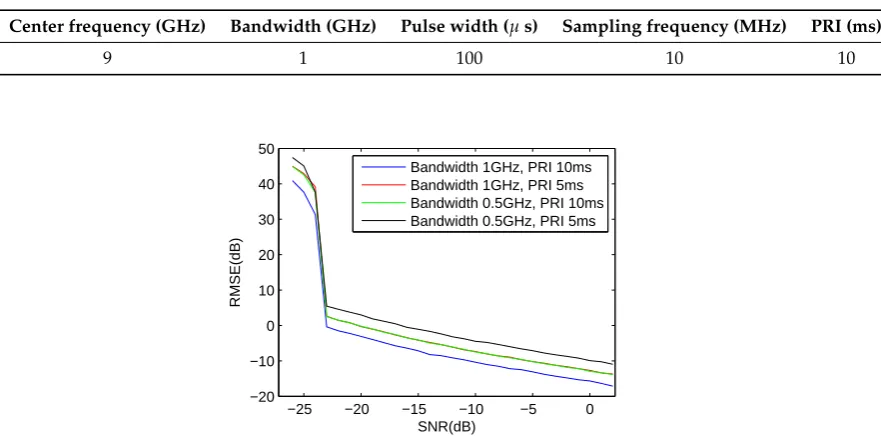
best performance. Under the same SNR, the RMSE performance of the case withB=1 GHz,Tpr =10
ms is about 3 dB lower than the case withB=0.5 GHz,Tpr =10 ms and the case withB=1 GHz and
Tpr =5 ms. The performance difference is about 6 dB between the case withB=1 GHz,Tpr =10 ms
and the case withB=0.5 GHz,Tpr=5 ms.
Table 3.Simulation Parameters of the Comparison with the ACCF Method.
Center frequency (GHz) Bandwidth (GHz) Pulse width (µs) Sampling frequency (MHz) PRI (ms)
9 1 100 10 10
−25 −20 −15 −10 −5 0
−20 −10 0 10 20 30 40 50
SNR(dB)
RMSE(dB)
Bandwidth 1GHz, PRI 10ms Bandwidth 1GHz, PRI 5ms Bandwidth 0.5GHz, PRI 10ms Bandwidth 0.5GHz, PRI 5ms
Figure 5.The performances of the proposed CCAE method with different parameters
4.2. Comparison with ACCF method
In this subsection, we compare the performance of the proposed CCAE method with the ACCF method [22,23] at different SNRs, which varies from -30 dB to 2 dB. 1000 Monte carlo simulations are also carried out for each SNR condition. The other simulation parameters are listed in Table3. In our simulations, the stretched signals are used in the proposed CCAE method, and the UR signals are used in the ACCF method, which can only be applied to the UR signals.
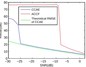
We first evaluate the performance of the case, in which only velocity is taken into account. The velocity of the target is set to 100 m/s. Two pulse echoes are used for only velocity estimation. In Figure 6, it is seen that the estimated RMSE of the proposed CCAE method outperforms that of the ACCF method. In addition, the estimated RMSE of the proposed CCAE method is close to the theoretical RMSE, which indicates that the error induced by the noise approximation ofω1(t,tm)ω1(t,tm+1)in section3.4is small.
We further evaluate the performances of the two methods with a second-order motion model. The velocity of the target is 100 m/s, and the acceleration is 10 m/s2. Three pulses are used for velocity and acceleration estimation, the other parameters being the same as those of the previous experiments. The estimated acceleration results are shown in Figure7, from which we can see that the RMSE of the CCAE method is much lower than that of the ACCF method. As has already been analyzed in section 3.4, SNR decreases after cross-correlation. To estimate the acceleration, the conjugate multiplication has to be used twice in the ACCF method, but only once in the CCAE method. Therefore, the performance loss is more in the ACCF method than in the CCAE method.
of velocity estimation of the ACCF method also becomes worse. In addition, for the proposed method, the RMSEs of the estimated acceleration and velocity are both close to the theoretical RMSEs, which proves the effectiveness of the proposed method. From a comparison of Figure6and Figure8, for the proposed CCAE method, it can be seen that the RMSE of the estimated velocity with acceleration is a bit higher than that without acceleration. This is because the velocity is calculated by subtracting two i.i.d variables. This can be confirmed by comparing equation (29) and (31).
−30 −25 −20 −15 −10 −5 0
−20 −10 0 10 20 30 40 50 60
SNR(dB)
RMSE(dB)
CCAE ACCF
Theoretical RMSE of CCAE
Figure 6.Comparison of RMSE results of the velocity estimation by using CCAE and ACCF methods (without acceleration)
−300 −25 −20 −15 −10 −5 0
10 20 30 40 50 60 70 80
SNR(dB)
RMSE(dB)
CCAE ACCF Theoretical RMSE of CCAE
Figure 7. Comparison of RMSE results of the acceleration estimation by using CCAE and ACCF methods (with acceleration)
−30 −25 −20 −15 −10 −5 0
−20 −10 0 10 20 30 40 50 60
SNR(dB)
RMSE(dB)
CCAE ACCF Theoretical RMSE of CCAE
The total time costs of the 1000 Monte carlo simulations for all the SNR cases are listed in Table 4. It is seen that the time cost of the proposed CCAE method is much smaller than that of the ACCF method. The reason is two-fold: first, the data size of the UR signal is larger than the stretched signal; second, the number of FFT operation required by the ACCF method is more than that of the CCAE method.
Table 4.Comparison of the Time Cost between CCAE and ACCF
Time cost (s) CCAE ACCF
Estimation without acceleration 81.6 5282.1 Estimation with acceleration 156.5 10175.3
Simulation environment: CPU frequency 3.30 GHz, memory 8 GB.
4.3. Verification with Real Data
Two sets of real data, obtained from the wideband LFM radar systems are applied for the verification of the proposed method. The parameters of the two data sets are shown in Table5. The targets are satellites. Figure9(a) and Figure10(a) show the estimated velocities in comparison with the real velocities of the targets. The errors between the estimated velocities and the real velocities of the targets are shown in Figure9(b) and Figure10(b). It is seen that the estimated results are consistent with the real velocities for both the data sets. The RMSE of the estimated velocity is 0.0561 m/s in the first data set and 0.2842 m/s in the second data set.
Table 5.Parameters of Radars.
Parameters Radar 1 Radar 2
Center Frequency (GHz) 9 3.2 Bandwidth (MHz) 2000 300 Sampling Frequency (MHz) 10 10
Pulse Width (µs) 400 200
PRI (ms) 40 100
0 10 20 30 40 50 60
−2000 −1500 −1000 −500 0 500 1000 1500 2000
Time (s)
Velocity (m/s)
Target’s real velocity Estimated velocity
(a)
0 10 20 30 40 50 60
−0.5 0 0.5
Time (s)
Velocity error (m/s)
(b)
0 20 40 60 80 100 −2000
−1000 0 1000 2000
Time (s)
Velocity (m/s)
Target’s real velocity Estimated velocity
(a)
0 20 40 60 80 100
−2 −1 0 1 2
Time (s)
Velocity error (m/s)
(b)
Figure 10.Estimation results of data set 2. (a) The estimated velocity and real velocity of the target. (Due to the high speed of the target and the high precision of the estimated velocity, the two lines overlap). (b) The error between the estimated velocity and the target’s real velocity.
Finally, the proposed CCAE method is applied to range alignment in ISAR imaging procedure, with a civil aircraft as the target. Figure11(a) shows the range profile with RM, caused mainly by the target’s velocity. Thus, it can be corrected by compensating the estimated velocities in the range profile. The result of range alignment, obtained by using the proposed method, is shown in Figure 11(b), from which it can be seen that the RM effect is eliminated, resulting in a focused ISAR image (Figure12). These results with real data demonstrate that the proposed method is effective in practical radar systems.
Range cell
Pulse number
500 1000 1500 2000
100
200
300
400
500
(a)
Range cell
Pulse number
500 1000 1500 2000
100
200
300
400
500
(b)
Figure 11.The range profile of the target. (a) The range profile with RM effect. (a) The range profile after range alignment by the proposed CCAE method.
Range (m)
Cross range (m)
−20 −10 0 10 20
−20
−15
−10
−5
0
5
10
15
20
5. Conclusion
In this paper, a new fast motion parameters estimation method based on CCAE for wideband LFM radars is presented. First, the conjugate multiplication is performed on the adjacent two signals. Then the velocity is obtained by estimating the frequency of the signal, i.e., the correlation result. The acceleration can be estimated by using three echo signals. The proposed CCAE method can be applied to the UR signals or the stretched signals. When estimating the velocity using two echo signals, the FFT operation is required only once in the proposed method, and the estimated parameters can be output in real time. Simulation results show that the new method provides better RMSE performances than the state-of-the-art existing method for both velocity and acceleration estimation, with much less computational cost. Besides, the RMSEs of the simulation data are close to the theoretical RMSEs of the proposed method. Real radar data sets are also evaluated to verify the effectiveness of the proposed method. The proposed fast estimation method of motion parameters can be applied to range alignment in ISAR imaging.
Acknowledgments:The research was supported by the National High-tech R&D Program of China, the Open-End Fund National Laboratory of Automatic Target Recognition (ATR), the Open-End Fund of BITTT Key Laboratory of Space Object Measurement and the National Natural Science Foundation of China (Grant No. 62101196).
Author Contributions: Yi-xiong Zhang, Zhen-miao Deng and Cheng-Fu Yang conceived and designed the experiments; Ru-jia Hong performed the experiments; Yun-jian Zhang analyzed the data; Cheng-Fu Yang and Sheng Jin contributed reagents/materials/analysis tools; Yi-xiong Zhang and Ru-jia Hong wrote the paper; Yi-xiong Zhang, Zhen-miao Deng and Cheng-Fu Yang modified the paper.
Conflicts of Interest: The authors declare that the grant, scholarship and/or funding mentioned in the Acknowledgments section do not lead to any conflict of interest. Additionally, the authors declare that there is no conflict of interest regarding the publication of this manuscript.
References
1. Skolnik, M.I. Introduction to radar.Radar Handbook1962,2.
2. Werness, S.A.; Carrara, W.G.; Joyce, L.; Franczak, D.B. Moving target imaging algorithm for SAR data. IEEE Transactions on Aerospace and Electronic Systems1990,26, 57–67.
3. Chen, V.C.; Qian, S. Joint time-frequency transform for radar range-Doppler imaging. IEEE Transactions on Aerospace and Electronic Systems1998,34, 486–499.
4. Berizzi, F.; Mese, E.D.; Diani, M.; Martorella, M. High-resolution ISAR imaging of maneuvering targets by means of the range instantaneous Doppler technique: modeling and performance analysis. IEEE Transactions on Image Processing2001,10, 1880–1890.
5. Yu, J.; Xu, J.; Peng, Y.N.; Xia, X.G. Radon-Fourier transform for radar target detection III: optimality and fast implementations.IEEE Transactions on Aerospace and Electronic Systems2012,48, 991–1004.
6. Suo, P.C.; Tao, S.; Tao, R.; Nan, Z. Detection of high-speed and accelerated target based on the linear frequency modulation radar. IET Radar, Sonar & Navigation2014,8, 37–47.
7. Peng, S.B.; Xu, J.; Peng, Y.N.; Xiang, J.B. Parametric inverse synthetic aperture radar manoeuvring target motion compensation based on particle swarm optimiser. IET radar, sonar & navigation2011,5, 305–314. 8. Chen, C.C.; Andrews, H.C. Target-motion-induced radar imaging. IEEE Transactions on Aerospace and
Electronic Systems1980,16, 2–14.
9. Wang, Y.; Ling, H.; Chen, V.C. ISAR motion compensation via adaptive joint time-frequency technique. IEEE Transactions on Aerospace and Electronic Systems1998,34, 670–677.
10. Wang, J.; Kasilingam, D. Global range alignment for ISAR.IEEE Transactions on Aerospace and Electronic Systems2003,39, 351–357.
11. Li, J.; Wu, R.; Chen, V.C. Robust autofocus algorithm for ISAR imaging of moving targets.IEEE Transactions on Aerospace and Electronic Systems2001,37, 1056–1069.
12. Wu, H.; Grenier, D.; Delisle, G.Y.; Fang, D.G. Translational motion compensation in ISAR image processing. IEEE Transactions on Image Processing1995,4, 1561–1571.
14. Xi, L.; Guosui, L.; Ni, J. Autofocusing of ISAR images based on entropy minimization.IEEE Transactions on Aerospace and Electronic Systems1999,35, 1240–1252.
15. Xu, J.; Yu, J.; Peng, Y.N.; Xia, X.G. Radon-Fourier transform for radar target detection, I: generalized Doppler filter bank. IEEE Transactions on Aerospace and Electronic Systems2011,47, 1186–1202.
16. Xu, J.; Xia, X.G.; Peng, S.B.; Yu, J.; Peng, Y.N.; Qian, L.C. Radar maneuvering target motion estimation based on generalized Radon-Fourier transform. IEEE Transactions on Signal Processing2012,60, 6190–6201. 17. Perry, R.; Dipietro, R.; Fante, R. SAR imaging of moving targets. IEEE Transactions on Aerospace and
Electronic Systems1999,35, 188–200.
18. Zhu, D.; Li, Y.; Zhu, Z. A keystone transform without interpolation for SAR ground moving-target imaging. IEEE Geoscience and Remote Sensing Letters2007,4, 18–22.
19. Li, G.; Xia, X.G.; Peng, Y.N. Doppler keystone transform: an approach suitable for parallel implementation of SAR moving target imaging. IEEE Geoscience and Remote Sensing Letters2008,5, 573–577.
20. Zhu, D.; Wang, L.; Yu, Y.; Tao, Q.; Zhu, Z. Robust ISAR range alignment via minimizing the entropy of the average range profile.IEEE Geoscience and Remote Sensing Letters2009,6, 204–208.
21. Li, Y.; Xing, M.; Su, J.; Quan, Y.; Bao, Z. A new algorithm of ISAR imaging for maneuvering targets with low SNR.IEEE Transactions on Aerospace and Electronic Systems2013,49, 543–557.
22. Li, X.; Cui, G.; Yi, W.; Kong, L. A fast maneuvering target motion parameters estimation algorithm based on ACCF.IEEE Signal Processing Letters2015,22, 270–274.
23. Li, X.; Cui, G.; Kong, L.; Yi, W. Fast Non-Searching Method for Maneuvering Target Detection and Motion Parameters Estimation. IEEE Transactions on Signal Processing2016,64, 2232–2244.
24. Lv, X.; Bi, G.; Wan, C.; Xing, M. Lv’s distribution: principle, implementation, properties, and performance. IEEE Transactions on Signal Processing2011,59, 3576–3591.
25. Luo, S.; Bi, G.; Lv, X.; Hu, F. Performance analysis on Lv distribution and its applications. Digital Signal Processing2013,23, 797–807.
26. Li, X.; Kong, L.; Cui, G.; Yi, W.; Yang, Y. ISAR imaging of maneuvering target with complex motions based on ACCF–LVD.Digital Signal Processing2015,46, 191–200.
27. Shui, P.L.; Xu, S.W.; Liu, H.W. Range-spread target detection using consecutive HRRPs.IEEE Transactions on Aerospace and Electronic Systems2011,47, 647–665.
28. Abatzoglou, T.J. A fast maximum likelihood algorithm for frequency estimation of a sinusoid based on Newton’s method.IEEE Transactions on Acoustics, Speech and Signal Processing1985,33, 77–89.
29. Xia, X.G. A quantitative analysis of SNR in the short-time Fourier transform domain for multicomponent signals.IEEE Transactions on Signal Processing1998,46, 200–203.
30. Xia, X.G.; Chen, V.C. A quantitative SNR analysis for the pseudo Wigner-Ville distribution. IEEE Transactions on Signal Processing1999,47, 2891–2894.
31. O’Donoughue, N.; Moura, J.M.F. On the Product of Independent Complex Gaussians. IEEE Transactions on Signal Processing2012,60, 1050–1063.