Reduction of the parameter estimation time for an adaptive control system

R E D U C T I O N O F T H E P A R A M E T E R E S T I M A T I O N

TIME FOR AN ADAPTIVE CONTROL SYSTEM

A Thesis submitted for examination for

the Degree of Master of Engineering ( Electrical) Dept. of Electrical & Electronic Engineering Faculty of Engineering

Victoria University of Technology (Footscray Campus) Victoria

Australia

1994

By

Robert V.Ives B.Sc.(Hons)

University of Nottingham Nottingham

FTS THESIS

629.836 IVE

30001004590354

Ives, Robert V

S Y N O P S I S

The following work is concerned with the use of the Method of Least Squares in the

parameter estimation of a discrete-time model of a system. In particular, the emphasis is upon both the initial convergence and accuracy of the estimates. The investigation is therefore pertinent to both the "cold-starting" of least squares estimators, and to systems in which "jump" changes in parameters occur, requiring resetting of the estimator.

The work was approached from an engineering viewpoint, with the requirement that

the theory be applied to a real system. The real system selected was a positional servosystem, using a DC motor.

A number of least squares algorithms were compared for their suitability to such an application. The algorithms examined were:

1) A standard, non-recursive solution of the least squares equations by Lower-Upper Factorisation of the information matrix.

2) A standard, recursive solution, i.e. Recursive Least Squares, RLS.

3) Two reduced order solutions using a priori knowledge of the type number of the servosystem (LU Factorisation and RLS).

4) An Extended Least Squares Solution, using a recursive algorithm. 5) Several non-recursive solutions using instrumental variables.

The methods were initially examined using a software simulation of the servosystem.

This simulation was based on a linear, second-order model. It was concluded that the preferred methods were the reduced-order solutions using a priori knowledge.

The following hypothesis was examined:

By raising the rate at which the signals are sampled, more information is

T h e simulation results indicated that the effect of sampling rate upon the quality of the estimate is different for the "Moving Average" coefficients, than for the "Auto-regressive" coefficients. For the noise model used in the simulations, an increase in sampling rate was found to improve the estimates of the "Auto-regressive" coefficients. Subsequent results, from measurements on the real system, showed that there is an upper sampling rate which should not be exceeded.

A real, positional servosystem was designed and constructed. Full details of this design are presented in the appendices of this thesis. The preferred algorithms, using a priori knowledge of the servosystem type number, were used to estimate the location of the unknown system pole. This pole was estimated using a number of different sampling rates. It was noted that the estimates deteriorated as the sampling rate was raised beyond a certain value. This was attributed to the decrease in signal to noise ratio with the increase in sampling rate.

All of the calculations and control were performed using a T800 Transputer. All

CONTENTS

SYNOPSIS » CONTENTS "i

CHAPTER 1 INTRODUCTION 1

1-1 INTRODUCTION TO SYSTEM IDENTIFICATION AND PARAMETER ESTIMATION 1

The Uses of System Identification

1-2 THE PROBLEM INVESTIGATED IN THIS THESIS 2 1-3 METHODOLOGY • 4

CHAPTER 2 LITERATURE REVIEW OF PARAMETER ESTIMATION USING THE METHOD OF LEAST SQUARES 6

CHAPTER 3 DESCRIPTION OF THE POSITIONAL SERVOSYSTEM 10 3-1 DESIGN AND CONSTRUCTION OF THE SERVOSYSTEM .... 10 The Drive Section of the Servosystem

The Measurement Section of the Servosystem

3-2 MODELLING OF THE DC PERMANENT MAGNET MOTOR .. 12 3-3 NON-LINEAR CHARACTERISTICS OF REAL DC MOTORS ... 14 Non-Linear Torque-Armature Current Characteristic

Cogging

Temperature Variations

Demagnetisation of the Permanent Magnets Non-Linear Friction-Angular Velocity Characteristic Summary

Static Friction Coulomb Friction

Solid Friction Models Summary

3-5 MODELLING THE PULSE WIDTH MODULATOR CONTROLLED MOTOR - STEADY STATE BEHAVIOUR 21

Introduction

An Equivalent Circuit for the Armature Winding and its Supply Derivation of the PWM Steady-State Model

3-6 MODELLING THE PULSE WIDTH MODULATOR CONTROLLED MOTOR - DYNAMIC BEHAVIOUR 26

Determination of the Component Values of the Equivalent Circuit of the Armature Winding

PSpice Simulations of the Equivalent Armature Circuit A Disturbance Model of the Armature Current

Spectral Content of the Disturbance Signal as a Function of PWM Duty-Cycle The Influence of the Worst Case Disturbance upon Motor Speed

Final Simple Model of the PWM Controlled Armature Current CHAPTER 4 PARAMETER ESTIMATION OF A DISCRETE-TIME MODEL OF THE SERVOSYSTEM 38

4-1 DEVELOPMENT OF A DISCRETE-TIME, INPUT-OUTPUT MODEL OF THE SERVOSYSTEM 38

The Need for a Discrete-Time Model Z Transform Notation

ESTIMATION

₄₂

EQUATIONS 44

4-4 A RECURSIVE SOLUTION TO THE LEAST SQUARES EQUATIONS 46

The Need for Recursive Algorithms

Young's Approach to a Recursive Algorithm

CHAPTER 5 COMPARISON OF DIFFERENT SOLUTIONS OF THE LEAST SQUARES EQUATIONS 50

5-1 REVIEW OF SOME ALTERNATIVE METHODS OF SOLUTION . .50 Some Direct Methods of Solution

Cramer's Rule, Gaussian and Gauss-Jordan Elimination LU Factorisation

Iterative Methods of Solution

5-2 BASES OF COMPARISON OF LU FACTORISATION AND RLS METHODS 52

Factors Affecting the Selection of the Preffered Method The Selection of Computer Simulation as the Basis of the Comparison

Some Comments on the Simulation Programs Computation Time

Rate of Convergence of Estimates Bias of the Estimates

Sensitivity of the Estimators to noise Richness of the Input Signal

Sampling Period of the Estimator Stability of the Estimator

5-3 THE COMPARISON OF LU FACTORISATION AND RLS METHODS USING A STOCHASTIC INPUT SIGNAL AT A STANDARD SAMPLING RATE 59

Results of the Simulations Computation Time

Rate of Convergence of Estimates Bias of the Estimates

Sensitivity of the Estimators to Noise Richness of the Input Signal

Sampling Period of the Estimator Stability of the Estimator

Summary of Simulations Using a Stochastic Input Signal and Estimator with Sampling Period of 0.2 Seconds

5-4 THE COMPARISON OF LU FACTORISATION AND RLS METHODS USING A STOCHASTIC INPUT SIGNAL WITH AN INCREASED SAMPLING RATE 68

Results of the Simulations

Rate of Convergence of Estimates

Sensitivity of the Estimators to Noise Richness of the Input Signal

Sampling Period of the Estimator

5-5 THE COMPARISON OF LU FACTORISATION AND RLS METHODS USING TEST INPUT SIGNALS 72

Test Input Signal Definitions Results of Simulations

Rate of Convergence of Estimates Richness of the Input Signal Sampling Period of the Estimator Stability of the Estimator

5-6 CONCLUSIONS OF THE COMPARISON OF THE LU FACTORISATION AND RLS METHODS 87

CHAPTER 6 A REDUCED ORDER ESTIMATOR USING A PRIORI KNOWLEDGE OF THE SYSTEM TYPE NUMBER 88

6-1 USE OF A PRIORI KNOWLEDGE OF PLANT INTEGRAL ACTION TO REDUCE THE ORDER OF THE ESTIMATOR 88

Introduction

Derivation of the Reduced Order Estimator

6-2 THE COMPARISON OF THE STANDARD AND REDUCED ORDER RLS METHODS OF SOLUTION 89

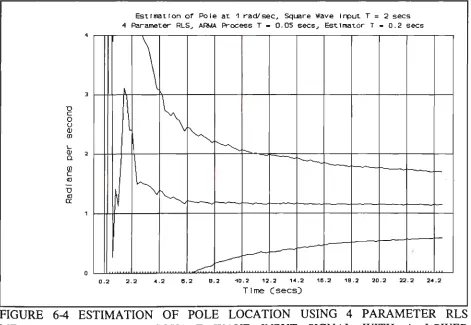
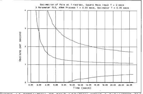
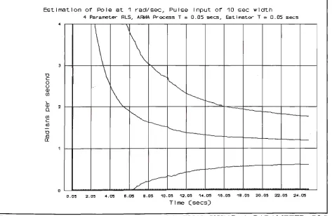
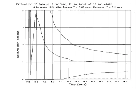
Description of the Simulations upon which this Comparison is Made Results of the Simulations Using the 3 & 4 Parameter RLS Methods Relative Merits of the Three and Four Parameter RLS Methods

CHAPTER 7 AN INVESTIGATION OF TWO TECHNIQUES INTENDED TO REDUCE THE ESTIMATOR BIAS 98

7-1 INTRODUCTION 98

7-2 SOURCE OF ESTIMATE BIAS 98

7-3 ESTIMATE BIAS AS A CONSEQUENCE OF CORRELATED NOISE 99

Introduction to the ELS Method

Computed Errors Based upon the Error in the One-Step Ahead Prediction

Computed Errors Based upon the Residual Sequence Results of the Simulations Using the ELS Method

Relative Merits of the 3 Parameter RLS and 6 Parameter ELS Methods 7-5 INSTRUMENTAL VARIABLE TECHNIQUES 108

Introduction to Instrumental Variables

The Ordinary IV Method as a Means of Reducing Estimate Bias Results of the Simulations Using Instrumental Variables

Relative Merits of the 3 Parameter RLS and 3 Parameter Instrumental Variable Methods

CHAPTER 8 THE APPLICATION OF THE THREE PARAMETER ESTIMATORS TO THE REAL SERVOSYSTEM 115

8-1 DESCRIPTION OF THE POSITIONAL SERVOSYSTEM 115 8-2 THE DETERMINATION OF THE LOCATION OF THE UNKNOWN SYSTEM POLE 115

Introduction

The Step Response of the Servosystem

8-3 USE OF THE THREE PARAMETER RLS ESTIMATOR WITHOUT MOTOR STOPPING OR REVERSAL 118

The Need to Avoid Motor Stopping or Reversal The Test Input Signal

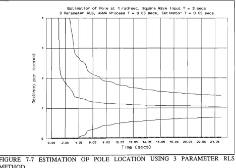
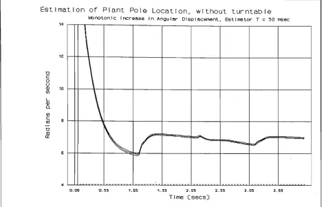
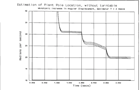
Results from the Three Parameter RLS Estimator without Motor Stopping or Reversal

or Reversal

Conclusion Drawn from the Above results

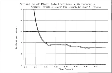
8-4 THE EFFECT OF INCREASED INERTIAL LOAD 125

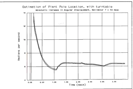
Results from the Three Parameter RLS Estimator on the System with Turntable, and without Motor Stopping or Reversal

Interpretation of the Results with Increased Inertial Load 8-5 THE USE OF THE THREE PARAMETER RLS ESTIMATOR WITH MOTOR REVERSALS 130

The Test Input Signal Used to Obtain Motor Reversals

Results from the Three Parameter RLS Estimator with Motor Reversals

Interpretation of the Results Using the RLS Estimator with Motor Reversals Conclusions Drawn from the Above Results

8-6 USE OF THE THREE PARAMETER LU FACTORISATION ESTIMATOR WITHOUT MOTOR STOPPING OR REVERSAL 137

The Reason for Reconsidering the LU Factorisation Algorithm The Experimental Set-Up

Results from the Three Parameter LU Factorisation Estimator without Motor Stopping or Reversal

Interpretation of the Results Using the LU Factorisation Estimator without Motor Stopping or Reversal

Conclusions Drawn from the Above Results

8-7 THE THREE PARAMETER LU FACTORISATION METHOD WITH INFORMATION MATRIX RESETTING 144

Introduction

Results of Using Information Matrix Resetting

Conclusions Concerning Information Matrix Resetting CHAPTER 9 CONCLUSIONS 149

9-1 INTRODUCTION 149

9-2 INVESTIGATION OF INCREASED SAMPLING RATE AS A MEANS OF REDUCING THE PARAMETER ESTIMATION TIME 149

Conclusions Based upon Measurements on the Real System Discussion Concerning the Simulations

Selection of Sampling Rate

9-3 USE OF INFORMATION MATRIX RESETTING TO IMPROVE THE NUMERICAL STABILITY OF PARAMETER ESTIMATORS ... 151 The Problem of Numerical Instability

The Preferred Solution

9-4 COMPARISONS OF DIFFERENT LEAST SQUARES ALGORITHMS 154

9-5 OBSERVATIONS ON THE USE OF A TRANSPUTER IN REAL-TIME DIGITAL CONTROL 156

APPENDDC A DESCRIPTION OF THE TRANSPUTER SYSTEM 158 A-l TRANSPUTER HARDWARE 158

A-2 TRANSPUTER SOFTWARE 158 Choice of Software Environment Programming Language

A-3 DYNAMIC SWITCHING OF THE SYSTEM CONFIGURATION . 160 Explanation of 'Dynamic Switching'

The Need for Dynamic Switching A-4 TIMING 162

B-l DESCRIPTION OF T H E C O M P L E T E POSITIONAL SERVOSYSTEM 163

B-2 THE PERMANENT MAGNET DC MOTOR 163 B-3 THE OPTICAL ENCODER 164

B-4 THE PLANETARY GEARHEAD 164

B-5 THE PULSE-WIDTH MODULATOR (PWM) UNIT AND POWER BRIDGE 172

B-6 THE INTERFACE CIRCUITRY 172

The Transputer Digital Interface Module The Digital-to-Analogue Converter (DAC) The Counter Circuit

The Counter Circuit Controller

Restrictions on the Counter Circuit Use

APPENDDC C NON-RECURSIVE SOLUTION OF THE LEAST SQUARES EQUATIONS 175

C-l THE SEQUENCE OF EQUATIONS NECESSARY TO SOLVE A FOUR PARAMETER PROBLEM USING LU FACTORISATION 175

Introduction

Sequence of Equations for LU Factorisation Solution - Four Parameter Case APPENDIX D PSPICE SIMULATIONS OF THE ARMATURE MODEL 178

APPENDIX E OCCAM2 SOURCE CODE OF THE SIMULATION PROGRAMS . 179

Source Code of the Method of Using A Priori Information to Reduce the Number of Normal Equations by One

Source Code for the Extended Least Squares Method

APPENDIX G 0 C C A M 2 SOURCE C O D E OF T H E P R O G R A M S USED T O TEST T H E REAL SERVOSYSTEM 194

Source Code Required to Perform Parameter Estimation of the Real Servosystem

Source Code Enabling Control of the B008 Motherboard Linkswitch REFERENCES 205

C H A P T E R 1 I N T R O D U C T I O N

lzl I N T R O D U C T I O N T O S Y S T E M I D E N T I F I C A T I O N A N D P A R A M E T E R ESTIMATION

EXPLANATION OF THE TERMS "SYSTEM IDENTIFICATION" AND "PARAMETER ESTIMATION"

System Identification may be viewed as the complete process by which an adequate

mathematical model of a real system is obtained [1-9]. A model may be derived either by the application of physical laws, or by the experimental observation of the system's response to known input signals. Usually both approaches are required in order to develop an accurate model.

Once the structure of the model is known, it then becomes necessary to determine the numerical values of the various parameters of that model. This process is referred to as Parameter Estimation.

In the following work, the system is modelled by a linear difference equation. The

justification of this model and the assumptions made in its derivation are given. Essentially this model, including its order, is derived from a consideration of the known components of the

system, and the laws of physics that these components must obey.

It is well known that the coefficients of such a difference equation may be estimated from a knowledge of the system components. Unfortunately not all characteristics of the components may be known with sufficient accuracy. The process of determining the optimum

numerical values of these coefficients is an example of Parameter Estimation. In the following work this process is achieved by using the model to predict the next output of the real system. The coefficients are estimated by adjusting them so as to minimise the summed square of the error in this prediction.

k n o w n as System Identification.

T H E U S E S O F S Y S T E M I D E N T I F I C A T I O N

In practice system identification is performed for one of two purposes.

The first is concerned with the understanding of the behaviour of a real system, as a

necessary prerequisite to the successful control of that system. From Kalman's earliest self-optimising controller [1-1] all self-tuning controllers have required the inclusion of some means of identifying the controlled system. Indeed, this feature of a distinct system identifier may be used in the definition of both self-tuning controllers and regulators [1-2].

The second use of system identification in engineering is in fault detection. Numerous

papers have been published on this aspect of system identification [e.g. 1-3,1-4,1-5]. Willsky [1-6] published a survey on the use of Kalman Filters, and related concepts, in the detection of system "failures".

\_1 THE PROBLEM INVESTIGATED IN THIS THESIS

The following work is concerned with the real-time parameter estimation of a

discrete-time model of a servosystem. In particular, the parameters are to be estimated as rapidly as possible, necessitating the calculations being based upon relatively few measurements. A

typical application of the system considered is the control of a turntable upon which a robotic arm has been mounted.

Such a system can be expected to exhibit behaviour predominantly dependent upon the

ratio of frictional losses to inertia of the rotating turntable. The model proposed is of second order, with one pole determined by this ratio, and the other associated with the integral action of converting angular velocity into angular displacement.

If the end-effector of the robot arm is moved further out, away from the axis of

the turntable will increase. F r o m a system identification viewpoint, this would cause a j u m p in the parameter values exhibited by the system. The controller of the turntable drive should be aware of these changes, in order to compensate for them.

The controller may contain a parameter estimator. In which case, after the jump

change in parameters this estimator should be reset, and a new set of estimates produced. The parameter estimator produces these new estimates from the sampled input and output signal sequences available after the jump change. The longer the length of these sequences the better (in terms of both increased information content and a consequent reduction in sensitivity to noise).

By increasing the sampling rate of these signals a larger number of signal pairs may be added to the sequences in any given, fixed time interval.

This thesis investigates whether or not such a simple technique can be used to improve

the estimation process. The intention is to perform the new parameter estimation using only the relatively few, post-jump measurements, rather than a long, cumulative history of probably irrelevant sampled values.

This approach was inspired by a consideration of an ideal, noise-free system of known

order. In such a deterministic case, a finite number of samples are required in order to exactly determine the values of the parameters. For a second-order, noise-free system, the difference equation relating the input and output signal sequences should have four coefficients. In the absence of noise, only four consecutive pairs of input-output signal samples should be required to determine the exact values of all four coefficients.

In a real system, all measured signals have associated noise. In addition no real,

discrete-time system can be precisely modelled by a linear, low order difference equation [1-7]. From the outset this approach was recognised as having a number of problems, e.g.:

Ill M E T H O D O L O G Y

The structure of the model of the system is assumed to be known, a priori. The

problem then is reduced to the determination of the numerical values of the parameters of that model.

The ideas and theory developed are aimed at one, real system. This system is a

positional servosystem using a permanent magnet DC motor. The armature current of this motor is controlled by a pulse-width modulated (PWM) amplifier. Details of the designs and construction of the hardware are given in Appendix B.

The models used to describe the servosystem were all input-output models. There was

no perceived advantage in using state-variable models. The work was restricted to techniques of parameter estimation based upon the Method of Least Squares.

A simple, linear model of the servosystem is proposed. The shortcomings of this model

are discussed. Particular emphasis is placed upon justifying the model of the PWM unit, and upon the non-linear characteristics expected of a real DC motor. The simple model is based upon the known (e.g. datasheet) characteristics of the components of the servosystem. This model formed the basis of a software simulation of the servosystem. A software simulation was used so as to permit the testing of parameter estimation algorithms without problems resulting from either an inadequate process model or an unknown noise process.

This approach ensured that the true coefficients of the system were calculable, and

hence available for comparison with the estimates. Testing the algorithms using either the real servosystem, or an analogue computer, would not have resulted in the availability of true

coefficient values. The use of software simulation overcame the problems of both inadequate modelling and component drift.

The simulations were used to compare two parameter estimation algorithms at a time.

Six algorithms were compared on the basis of their suitability to the specific task of

real-time parameter estimation of a second-order, type one system. The algorithms considered were:

i) Four parameter, non-recursive solution using Lower-Upper (LU) Factorisation ii) Four parameter solution using Recursive Least Squares (RLS) Method

iii) Reduced order (three parameter) solution using LU Factorisation iv) Reduced order (three parameter) solution using RLS

v) Six parameter Recursive Extended Least Squares Method

vi) Reduced order (three parameter) solution using instrumental variables.

The preferred algorithms (iii and iv) were tested on the real system for a number of sampling rates. The other four algorithms having exhibited inferior performance for this application in the comparisons based upon simulation were not used on the real system. The theoretically derived second-order model was assumed to be adequate to describe

the real system behaviour at all times. There was no attempt to define a restricted, linear region of operation of the servosystem. Two different input test signals were used on the real system. The first caused the motor to rotate continuously in the one direction. This was done to avoid the non-linear, unmodelled behaviour expected in both reversing and stopping the motor. The model used did not consider such effects as backlash and deadband. The second test signal caused the motor to be driven alternately in either direction. This enabled some observations to be made on the effects of these unmodelled non-linearities upon the estimator performance.

CHAPTER 2 LITERATURE REVIEW OF PARAMETER ESTIMATION USING

THE METHOD OF LEAST SQUARES

The first self-tuning controllers [1-1,2-1,2-2] were primarily intended for the control of systems with unknown, time-invariant parameters. These designs involved the minimisation of a selected Performance Index. Kalman and Koepcke [2-3] attributed the idea that control systems should be designed in such a way as to minimise a performance index based upon the integral of a squared error signal to Wiener.

The original development of the Method of Least Squares was done by Legendre and

Gauss, both publishing their work near the start of the nineteenth century [2-4]. These famous mathematicians independently developed this method to apply to batches of previously obtained astronomical measurements. The first recursive solution of the Least Squares Problem was published by Plackett [2-5]. This recursive approach was developed as a means of minimising the computation required if additional observations were to become available.

Kalman's early design of a self-optimising, discrete-time control system [1-1] used a

performance index consisting of the mean squared error in the prediction of the system's output signal. Stromer [2-6] published a brief bibliography covering the early work on self-optimising control systems.

The simple performance index has been extended by various authors into more

elaborate Cost Functions [e.g. 2-4]. Clarke and his co-workers [2-2,2-8] proposed cost functions that penalised control effort as well as output prediction error.

arithmetic. They are especially valued for dealing with the problem of "round-off" errors in computers of short word-length.

Graupe and his co-authors considered a number of different algorithms based upon the Method of Least Squares [2-12]. Their paper classified the algorithms into the following groups:

i) Batch least squares methods (including covariance, autocorrelation and partial correlation methods)

ii) Sequential least squares methods (including the standard Recursive Least Squares Method [2-13], and sequential forms of the covariance and partial correlation methods)

iii) Lattice algorithms

iv) Square Root algorithms (including the use of Householder Transformations) In their comparison the authors considered the convergence characteristics of each

method. They concluded that "the convergence and convergence-rate properties of different least-squares algorithms are almost identical for 36 or 64 bit accuracy".1

Of all the methods considered by Graupe and his colleagues, they nominated the

"Sequential Direct LS" approach, this is the same as that called Recursive Least Squares (RLS) in Chapter 4 of this thesis.

Wong and his co-authors [2-14] reported problems with numerical instability when

using the RLS method within an industrial application. This group favoured an algorithm based upon the Recursive U-D Factorisation Method [2-11]. It should however be noted that this choice was in response to the problem of "bursting" of the estimates [2-14]. This problem is prevalent when the estimator has a large set of past samples available to it. The present work considers the case of the estimator having few samples, and hence "bursting" is not a concern

in algorithm selection.

The application of self-tuning controllers to time-invariant, almost linear systems is now extensively covered in the literature. The problems of such designs and suggested

solutions being well documented, e.g. biased estimates resulting from coloured noise [2-15], lack of persistency of excitation [2-16].

The self-tuning controllers can be easily modified to produce adaptive controllers

suitable for systems with slowly time-varying parameters. Kalman, Swerling and Wittenmark [1-1,2-17,2-1] have all noted the ease by which this could be achieved.

In order to make a self-tuning controller adaptive, the most common modification is the introduction of an exponential weighting to discount previously measured values. This is achieved by scaling past data by a constant forgetting factor [2-18]. A number of authors have encountered problems when using a constant forgetting factor [e.g. 2-19,2-20]. Invariably the choice of this factor is empirical, ad hoc and crucial to the system performance and as a consequence, a number of schemes involving variable forgetting factors have been proposed [e.g. 2-18,2-22,2-23,2-24].

Gurubasavaraj [2-21] noted that an inappropriate choice of forgetting factor resulted in

"numerical instabilities". Gurubasavaraj found it necessary to supplement the use of a constant forgetting factor with some resetting of the covariance matrix. Others have also resorted to resetting the information or covariance matrix of the estimator [2-25], or the use of a cascade of estimators [2-26].

The choice between forgetting factor or matrix resetting is largely determined by the

rate at which the system parameters are able to change. The literature tends to consider two classes of parameter variation, commonly described as "drift" and "jump" changes. Goodwin and Teoh [2-27] provided a review of the literature on this problem up to 1983. They

simplest form, requires regular, periodic resetting of the covariance matrix. They suggest that in the case of "jumps" in parameter values, that there is some advantage in monitoring the prediction error as a basis for covariance resetting.

The choice of sampling period for parameter estimation of a real system must

inevitably be related to the time constant of that system. Commonly the sampling period is based upon either the closed loop bandwidth of the system [e.g. 5-13,5-14,5-15], or some other time constant of the system [e.g. 5-16]. Astrom and Wittenmark [2-28] provide an

introductory treatment of the selection of an appropriate sampling period. The parameter values are dependent upon the sampling period, and their sensitivity to error has been noted in both the selection of sampling period and choice of modeling operator [2-29].

Astrom [2-7] mentions that adaptive schemes derived from Stochastic Control Theory

C H A P T E R 3 D E S C R I P T I O N O F T H E P O S I T I O N A L S E R V O S Y S T E M

3-1

The following brief description of the real servosystem is included as an introduction to

the derivation and justification of a mathematical model of that system. A more comprehensive description of the design and construction is provided in Appendix B.

THE DRIVE SECTION OF THE SERVOSYSTEM

The servosystem uses an 18 volts, 40 watts, permanent magnet DC motor. This motor

is controlled by its armature current. The armature winding is supplied from a bridge of power, VMOS transistors. The transistors act as switches, as shown in Figure 3-1.

+

15V

A

9 o

o

() <>

C

ov

The transistors are alternately switched in opposite pairs. Initially, transistor switches A and D are open, with B and C closed. In this case the applied armature voltage will attempt to drive a positive conventional current through the winding from right to left.

Transistors B and C are subsequently turned-off also. For a brief period (nominally ten

microseconds) all four switches are open, to avoid shorting out the +15 volt supply. After this short period, switches A and D are closed. The applied armature voltage now attempts to drive positive conventional current through the winding from left to right, however the total current is dependent upon the voltage induced in the armature winding.

The switching cycle is then completed by a further short period when all four switches

are open. The complete cycle of four switching operations is repeated at a nominal, ultrasonic rate of 22KHz.

TABLE 3-1 SEQUENCE OF TRANSISTOR SWITCHING Period Number Switches A&D Switches B&C 1

2 3 4

The armature current is controlled by varying the ratio of Period 1 to Period 3. This

ratio is referred to here as the "cycle" of the pulse width modulator (PWM) Unit. A duty-cycle of 50% indicates that Periods 1 and 3 are of equal duration, resulting in an average armature current of zero.

The design of the PWM Unit is based upon two comparators fed with an internally

generated 22KHz. triangle wave and an input voltage, v.(t) . The input signal, vt(t) ,is

open open closed open

produced by a digital-to-analogue converter (DAC) connected to an output port of the digital

controller. Figure 3-2 shows the interconnection of the various circuit blocks of the Drive Section.

DIGITAL I l\

CONTROLLER—/

LATCH

& DAC

22 KHz

TRIANGLE

WAVE GEN

PWM

UNIT

HEXFET

BRIDGE

i

(0

FIGURE 3-2 B L O C K D I A G R A M O F T H E D R I V E CIRCUITS O F T H E S E R V O S Y S T E M

THE MEASUREMENT SECTION OF THE SERVOSYSTEM

The controlled output variable of the system was the angular position of the output

shaft of a gearbox driven by the motor armature shaft. Position measurements were made using

an optical encoder connected to the armature shaft. Details of this transducer, and its associated circuitry are given in Appendix B.

3-2

MODELLING OF THE DC PERMANENT MAGNET MOTOR

For simplicity a very simple, linear model of the D C motor was selected. The majority

The selected model is summarised in Figure 3-3, with the following terms as defined:

v.(0 ,

eb(.t) ,

m ,

w ( 0 , 8(0 ,

K •

K •

*,. ,

B ,

J ,

the applied armature voltage

the back emf of the armature winding the armature current

the torque developed by the armature the angular velocity of the armature the angular position of the armature

the resistance of the armature winding the inductance of the armature winding the motor torque constant

the viscous frictional coefficient for the rotating section of the machine the rotational inertia of the machine

the back emf constant

Capital letters denote Laplace Transforms, i.e. S£[i*a(0] = Ia(s)

V Q ( S )

+

(s)T(s)

K;

1

B + sJ

n(s)

Eb(s)

Kb

1 s

B(s)

The above model incorporates a number of assumptions:

1) that the armature winding may be treated as a single winding comprising of a series connection of a lumped resistance, lumped inductance and a dependent voltage source. This voltage source modelling the back emf induced in the winding.

2) that the back emf is directly proportional to the angular velocity of the armature.

3) that the torque developed by the armature is directly proportional to the armature current, and that all of this developed torque is available to overcome frictional losses and to accelerate the rotor, i.e.

7X0 = Bo>(0 + J— «(0 3-1

dt

There is no disturbance torque included in the model.

4) that the mechanical, frictional losses are viscous in nature. This assumption is reviewed in Section 3-3 below.

__l NON-LINEAR CHARACTERISTICS OF REAL DC MOTORS

Kuo and Tal [3-4] point to a number of inadequacies of the above model. These inadequacies are summarised below:

NON-LINEAR TORQUE-ARMATURE CURRENT CHARACTERISTIC

There are two sources of non-linearity in this characteristic.

ii) The second source of non-linearity is associated with the angular position of the armature with respect to the stator. This effect is noticeable if the motor has an insufficient number of commutation points and manifests itself as a cyclical variation of torque It may be modelled as a cyclical torque disturbance.

COGGING

The reluctance of the magnetic circuit may vary with the angular position of the rotor. The rotor will then have preferred, stationary shaft-angle positions. At low speeds the rotor may be observed to "cog".

TEMPERATURE VARIATIONS

Arguably the most significant problem with temperature changes is the dependence of the relative permeability of the motor's magnetic materials upon temperature.

DEMAGNETISATION OF THE PERMANENT MAGNETS

Excessive currents may demagnetise the permanent magnet, resulting in an irreversible change in the characteristics of the motor.

NON-LINEAR FRICTION-ANGULAR VELOCITY CHARACTERISTIC

The viscous damping coefficient of the motor is not a constant. There are a number of

SUMMARY

Of the above non-linear characteristics it was expected that the most significant would

be the non-linearity of the frictional losses. The other non-ideal characteristics were considered to be either of a secondary nature or avoidable. An high quality motor was purchased, so as to minimise the significance of the above characteristics.

The assumption concerning the non-linearity of the frictional losses however, had the potential to discredit the whole of the model. Accordingly the following section provides a

brief overview of the literature and available models describing frictional losses appropriate to DC motors.

34 REVIEW OF FRICTIONAL LOSSES

The literature concerning frictional losses in DC motors suggests that a general model,

based on physical principles, is not available. Instead there exist a variety of empirical models, which tend to be specific to either certain modes of motor operation, or types of motor

construction.

SLIDING VS. ROLLING FRICTION

Bowden and Tabor [3-20] provide an insight into why diverse models are able to

co-exist. The underlying physical processes that manifest themselves as either "sliding friction" or "rolling friction" are entirely unrelated. Accordingly a motor constructed with ball-bearings would have a different speed-friction characteristic from one constructed using simple journal bush bearings.

VISCOUS FRICTION

The model of the motor proposed in Section 3-2 considered that the frictional

Tft) = B—0(0 3-2

is the frictional component of shaft torque is the angular position of the shaft

is the Viscous Frictional Coefficient [3-4]

For the model of Section 3-2 the Viscous Frictional Coefficient is a constant. A linear relationship between frictional torque and shaft speed implies a quadratic

relationship between the frictional power loss and shaft speed. Puchstein [3-6] gives empirically based equations for determining the power loss in small DC motors, operated at constant

speed. He suggests that the power loss due to bearing friction and windage is proportional to the armature speed raised to the power of 1.5. Kuo and Tal [3-5] state that not all components of the viscous damping effect are linearly related to angular velocity.

The distinction between the terms viscous frictional coefficient and viscous frictional constant is therefore important.

STATIC FRICTION

Static Friction is a component of friction associated with stationary surfaces only.

Ts(f) = ±r0|6=0 3-3

where

Ts(t) , is the torque due to Static Friction

T0 , is an empirically obtained constant 0 , is the angular velocity of the shaft where

T/t)

8(0

K u o & Tal [3-4] wrote that "once motion begins, the static frictional force vanishes, and other frictions take over".

B o w d e n & Tabor [3-20] differentiate between the "Coefficient of Static Friction" and the "Coefficient of Kinetic Friction". These authors give three reasons w h y the Coefficient of Static Friction should be the larger:

i) Stationary surfaces will probably be in better contact with one another

ii) Over a period there m a y be contact diffusion of atoms from the material of one surface to that of the other

iii) A n y thin film, that would serve as a lubricant between the two surfaces, m a y break down.

COULOMB FRICTION

Classical models of Friction recognise a third type of friction, k n o w n as Coulomb

Friction. The torque due to Coulomb Friction, T(t) , is given by:

Tc(t) = Tv

d6

dt

_3-4

de

dt

where

Tx , is an empirically obtained constant.

The physical justification of Coulomb Friction is to model the magnetic and mechanical

hysteresis associated with reversals of direction of motor rotation [3-8]. The effect of Coulomb Friction in real systems is to reduce overshoot and oscillations, at the expense of steady-state error [3-4].

S O L I D F R I C T I O N M O D E L S

Some authors have noted that models of friction based upon Viscous, Coulomb and

Static components, fail to describe the behaviour of real systems [3-9,3-10,3-13]. A more elaborate model, the Solid Friction Model, has been developed to overcome these failures. This new model has been subject to several developments and simplifications [3-9,3-10,3-12].

The Solid Friction Model is the result of finding a mathematical function that will fit an experimentally obtained curve. Unfortunately the resulting function is both unwieldly and non-linear:

dF(x)

dt

S.a

dt

3-5

where

F(x), x,

i, a and F,

S,

is the Frictional Force is the displacement

are constants, chosen so as to enable the function to fit the required curve

is a "Stability Factor" [3-11]

Dahl has used the Solid Friction Model to represent a system comprising of a D C

motor, gearbox and inertial load [3-11]. This paper reveals the complexity involved in using the Solid Friction Model.

Tp) + x . — j ^ = (sgn k).Te 3-(

is the predicted frictional torque

is the constant rolling friction torque

equals either + 1 or -1, depending upon the sign of the relative gimbal velocity

is a suitably chosen constant

SUMMARY

There exist two groups of models of friction appropriate to the positional servosystem considered in the present work.

The first group is based upon the "classical" components of friction, namely Viscous, Coulomb and Static. Various combinations of these components m a y be used, depending upon the operational m o d e of the motor considered. A combination of the Viscous and C o u l o m b components proving adequate to m a n y authors [e.g. 3-7,3-14].

The second group of models are those derived from Dahl's Solid Friction Model. The model of Section 3-2 uses a simple model consisting of viscous friction alone. Further, the Coefficient of Viscous Friction was taken to be a constant. This selection was made since it is so simple. T h e above review of friction indicates the level of confidence that can be placed on this choice. H o w e v e r it would not be sensible to choose a m o r e complex model, before the arrival of experimental results makes the use of such a model imperative.

The above overview of friction suggests that different models are necessary for different modes of motor operation, i.e.

i) rotation continuously in one direction with only slight speed variations where

Tff) ,

ii) rotation continuously in one direction with a wide range of speeds or iii) motion subject to either stopping or reversals of direction of rotation.

3;5 MODELLING THE PULSE WIDTH MODULATOR CONTROLLED MOTOR -STEADY STATE BEHAVIOUR

INTRODUCTION

The model of Section 3-2 showed the applied armature voltage as the input signal to the system. The real system has this voltage generated by a Pulse Width Modulator (PWM) controlled bridge of power transistors. This circuit is not linear, its output voltage being a

variable duty-cycle train of rectangular pulses.

The following sections, 3-5 and 3-6, provide an analysis of the effects of this circuit on the armature current, and are a justification of the simple, linear model given as Equation 3-39.

AN EQUIVALENT CIRCUIT FOR THE ARMATURE WINDING AND ITS SUPPLY

The bridge of power transistors supplies a variable duty-cycle, fixed frequency, +/- 15 volts, rectangular wavetrain across the terminals of the armature winding. This wavetrain is modelled by two, synchronised, independent voltage sources, as shown in Figure 3-4. In practice there must be a deadtime during which both vt(f) and v2(0 are zero, however to simplify the following analysis the deadtime is assumed to be zero.

'aCO

R

a

L

a

c

o h ^

m

R

_m

<$r

e

_b

(t

6f

V

2(

t

FIGURE 3-4 CIRCUIT DIAGRAM USED TO MODEL THE SWITCHING OF THE

APPLIED ARMATURE VOLTAGE

*

1 «

Vc

(D k

V

(t)

Vc

CD

FIGURE 3-5 W A V E F O R M S U S E D T O G E N E R A T E T H E A P P L I E D A R M A T U R E

V O L T A G E

In Figure 3-4 the back-emf is considered to be the voltage developed across a parallel

R-C circuit, rather than the more conventional use of either an independent or dependent

The model of Section 3-2 includes the following relationships: 71(0 - ktia(t) 3-7

7X0 = Sw(0 + J—w(0 3-8

dt

eb(t) = kbu>(t) 3-9

and therefore

Thus the back-emf may be modelled as the voltage developed across a parallel R-C circuit, as per Figure 3-4, where:

K = — Ohms 3-11

M Q

and

C = — Farads 3-12 k}cb

The time constant of this circuit is equal to the Mechanical Time Constant of the motor.

D E R I V A T I O N O F T H E P W M S T E A D Y - S T A T E M O D E L

The following sub-section of this work derives a steady-state relationship between the average armature current and the duty-cycle of the PWM Unit.

The following assumptions are made:

i) the PWM duty-cycle has been held at a constant value

ii) the load presented to the motor shaft is a constant torque. As a consequence of these assumptions:

iii) variations in o>(0, and hence eb(t) are sufficiently small as to permit

Assumption iii) relies on the Mechanical Time Constant of the motor being much greater than the time period of the P W M switching cycle. This assumption effectively ensures that the charge on the capacitor Cm remains constant throughout the period of the P W M

switching cycle. The back-emf then becomes the voltage developed across the resistor Rm, with

the capacitor replaced by an open-circuit, i.e.

e

*C) = *JJ®

"

The armature winding then exhibits a total resistance, R, where

R = R+ R 3-14 a m

Over the first part of the P W M cycle, 0<t<kT, the armature current is given by:

3-15

ijt) ' ~M(t) +

H-fl

where u(t) denotes a unit step.

Hence at the end of this first period the instantaneous value of the armature current will be given by

ia(kT) = ^ +

Over the second part of the P W M cycle (kT < t < T) the voltage vt(0 is zero, and

v2(0 is now equal to +Ve volts.

Define x =t-kT , in which case the second part of the cycle may be described by the

range 0 < t < (1 -k)T- The initial current for this period may be described as

' r ' M ^ W U

3

"

17

Over this second period it can be shown that:

aK _{' R R °} .exp^

-Rx

Hence at the end of the P W M cycle it can be seen that:

' « O U = i«(T)U(i-t)r= ~ + —1+*„

R °

exp. -R(l -k)T\ 3-19 This equation is based on the assumption that the duty-cycle of the P W M is held

constant, and accordingly:

Hence it can be shown that the initial current is given by:

3-20

t „ v-R(\-k)T^ T-RT,

1 + 2 . e x p [ — - — ] -exp[ ]

w u - \i -

l - e x p [ — — ]

The average value of the armature current over the period Ozt<kT, IAV1, is given by:

£T

7?

, kIRs +

e x p ( — — ) - l

3-22

Similarly the average value of the armature current over the period kT<.t_T, IAV2 is

given by:

(i-*)r

IAV> - \ i£i)dt

« + '

R (l-k)T

Wl

n

L R &M

<tm*yi

IAVVkT+IAV2.{l-k)T

L

AV j J" ^

and hence

IAV = ^.(2*-l)

3 "25

This equation shows the linear relationship between the duty-cycle k, and the average (over one cycle of the PWM switching period) armature current. The expression is valid subject to the assumptions stated.

!£ MODELLING THE PULSE WIDTH MODULATOR CONTROLLED MOTOR -DYNAMIC BEHAVIOUR

In the foregoing analysis it was assumed that the duty cycle of the PWM drive was held constant and accordingly the dynamics of the motor were neglected. In this section the response to a change in duty-cycle will be considered. This response will be investigated by simulations using the software circuit analysis package "PSpice" [3-15,3-16]. The circuit simulated is that of Figure 3-4.

The simulation requires numerical values for the various components of the equivalent circuit. The following subsection justifies the values selected for use in the subsequent simulations.

DETERMINATION OF THE COMPONENT VALUES OF THE EQUIVALENT CIRCUIT OF THE ARMATURE WINDING

The component values were determined by use of data provided by the manufacturer of

motor. These fixtures will cause a difference to exist between the numerical values of

Rotational Inertia, J, and Coefficient of Viscous Friction, B, calculated here, and those to be expected of the real system.

The main purpose of this section of the work is to justify the use of a simple, linear

model of the PWM Unit. The validity of this justification is not lessened by the use of data for an unloaded motor.

The motor manufacturer provided the following data: Rotor inertia, J = 63.5 mg.m.m

Armature resistance, Ra = 0.747 Ohms

a

Armature inductance, La = 0.23 m H

Torque constant,fc. = 36.5 mN.m/A

No load current, 1^ = 387 raA (18 Volts Supply)

No load speed, o>0 = 4500 rpm (150 ^ radians per second)

These figures enabled the no load back emf, EM to be found :

EM = Va - 7^a = 17.7 Volts 3-26

The required value of the parallel resistance may be determined from the no-load information

/?=____„ 45.7 Q 3-27

I

1_a0

Similarly the value of the Back-Emf Constant,^ may be found

jfc

= __*? = J2_Z_ ~ 3.76. IO"

3-28

b

co0 150.it

e

(t).i

(t) = 7X0-co(0 3-29

This equation shows that the constants k. and k

have the same value. Many authors

[e.g. 3-18,3-19] simplify their analyses by the use of this approximation. Non-zero values for

the above losses requires the input power to be greater than the output power. This inequality

results in k

>k.. The value of k

obtained from Equation 3-28 is indeed slightly greater than

the datasheet value of k

.

The no-load data may be used to calculate the value of the Coefficient of Viscous

Friction, B. Since the no-load values are steady state values, then the armature is not subject to

acceleration. The Torque Equation , Equation 3-8, reduces to

:-7X0 = B.w(t) 3-30

and hence

B - L.— « 3.10"

Nm^ecs 3-31

The values obtained for k

and B, provide a second means of calculating the value of

the equivalent parallel resistance.

R - ______ = 36.5.1Q-

.3.756.1Q-

_

.

m

~ B 3.10"

which is consistent with the value obtained from Equation 3-27.

Further the equivalent parallel capacitance may be found

C = — = 6.35.10" = 46.3/nF 3-33

m

k^ 36.5.10"

.3.756.10-

PSPICE S I M U L A T I O N S O F T H E E Q U I V A L E N T A R M A T U R E CIRCUIT

The PSpice Circuit Simulation and Analysis software was used to examine the

The first PSpice simulation examined the step response of the armature model. The

input signal being a step in applied armature voltage from 0 volts to +15 volts. Figure 3-6 provides plots of the resulting armature current and back-emf.

20 +

"TlrAE

F I G U R E 3-6 PSPICE S I M U L A T I O N O F T H E A R M A T U R E C I R C U I T S T E P R E S P O N S E

The mechanical time constant of the motor model was obtained from Figure 3-6 by

Figure 3-7 shows the response of the armature model to the initial turn on of a 2 2 k H z pulse width modulated voltage supply. The traces are for duty cycles of 50%, 60%, 70% and

90%. Figure 3-7 shows the initial 2 milliseconds of the transient, a period far shorter than the mechanical time constant of the motor. The traces therefore effectively show the build up of the starting current resulting from the PWM turning on, prior to the back-emf achieving its steady-state value.

0.0ms 0.5ms 1.0ms 1.5ms 2.0ms

The traces of Figure 3-7 were used to measure the electrical time constant of the model

of the armature winding. Each trace is treated as if it consists of a mean armature current, onto which a 22 kHz sawtooth disturbance has been superimposed. The electrical time constant is

taken as the time taken for the mean current to reach 63 % of its final value.

From Figure 3-7, three different values of the electrical time constant were obtained, corresponding to the traces for duty-cycles of 90%, 70% and 60%. The respective time

constants being 0.28, 0.27 and 0.24 milliseconds. These values are slightly less than that

expected using the motor datasheet [4-3]. The datasheet values indicate that the electrical time constant, xe, should have a value given by:

L

-=-!•« 0.31 msecs 3-34

It is concluded that the average armature current changes at a maximum rate

predominantly determined by the Electrical Time Constant of the armature winding. Figure 3-8 is included to show that the simulations do subsequently show a fall in the

armature current as the back-emf is developed. This graph shows the first 10 milliseconds of the transient for the 90% duty cycle.

A DISTURBANCE MODEL OF THE ARMATURE CURRENT

The simple, linear model of the PWM Unit that is presently being justified uses the

above idea of the armature current being composed of an average value onto which a sawtooth disturbance waveform has been added. The disturbance waveform is an high frequency signal, formed from a 22 kHz fundamental and its harmonics. This disturbance signal is injected into a system which acts as a low pass filter. Consider the effect of the PWM duty cycle on the

spectral content of this disturbance signal.

Analysis shows that the disturbance signal is most significant for a duty-cycle of 50%.

signal is negligible.

16 +

0

Oms 2ms o i (ra) - v(3,4)

Time

FIGURE 3-8 PSPICE S I M U L A T I O N O F T H E A R M A T U R E T R A N S I E N T R E S P O N S E FOR PWM UNIT START-UP WITH A 90% DUTY CYCLE

Figure 3-9 shows a block diagram of the means of modelling the PWM Unit. The

applied armature voltage va(0, was considered to equal the mean value of the +/- 15 volt wavetrain from the PWM Unit. The 22 kHz switching frequency was modelled by an

The P W M Unit was thus modelled as a simple, gain block,k., where:

*_• =

v,(0

3-35

Vi(s

Vafs

->

+

-^

1

R + sL

Ebfs

+

A

al s

d(s

FIGURE 3-9 B L O C K D I A G R A M O F P W M U N I T M O D E L W I T H INJECTED A R M A T U R E D I S T U R B A N C E C U R R E N T

S P E C T R A L C O N T E N T O F T H E D I S T U R B A N C E S I G N A L A S A F U N C T I O N O F P W M DUTY-CYCLE

The duty-cycle of the PWM Unit affected both the amplitude and the waveshape of the

disturbance signal. This section identifies the 50% duty-cycle as being that at which the disturbance signal was most significant. At this duty-cycle the amplitude of the disturbance signal was at its largest value, this is in agreement with the traces of Figure 3-7.

The same PSpice simulations were used to investigate the spectral content of the

the power in the fundamental and first eight harmonics of a periodic waveform.

These results were obtained from the transient simulations presented in Figure 3-7, for the last cycle of the disturbance signal within the period covered by the simulation.

Accordingly it is acknowledged that the results are not true steady-state values, since these transient simulations terminate prior to the motor reaching its steady-state speed. The results are however, taken from a period well after the armature current has reached its maximum

value.

The selection of this period as the basis of the Fourier Analysis was made so as to avoid the need for a number of protracted transient analyses. The results of the Fourier Analyses are presented in Table 3-2.

The servosystem acts as a low pass filter. Accordingly the higher frequency harmonics

receive a greater attenuation than either the fundamental or low frequency harmonics. Table 3-2 shows, for the duty-cycles considered, that the fundamental carries most of the power of the disturbance signal. Table 3-2 also shows that as the duty-cycle is increased (i.e. moved further away from its base value of 50%) that the power at the fundamental frequency falls. These

T A B L E 3-2 E F F E C T O F P W M D U T Y - C Y C L E U P O N T H E R E L A T I V E P O W E R O F THE SWITCHING FREQUENCY FUNDAMENTAL AND ITS

HARMONICS

Frequency Component Duty Cycle 50% 60% 70% 90%

22 kHz Fundamental 0.5984 0.5682 0.4817 0.1797 2nd Harmonic 0.0000 0.0874 0.1415 0.0850

3rd Harmonic 0.0651 0.0378 0.0209 0.0507 4th Harmonic 0.0000 0.0342 0.0206 0.0329 5th Harmonic 0.0219 0.0002 0.0217 0.0214 6th Harmonic 0.0000 0.0139 0.0089 0.0138 7th Harmonic 0.0106 0.0062 0.0030 0.0082 8th Harmonic 0.0000 0.0043 0.0069 0.0044 9th Harmonic 0.0056 0.0052 0.0044 0.0019

THE INFLUENCE OF THE WORST CASE DISTURBANCE SIGNAL UPON MOTOR SPEED

Figure 3-7 shows that for a 50% duty-cycle, the disturbance signal has a peak-to-peak

value of approximately one Amp. The significance of this signal may be tested by replacing it by a sinewave disturbance signal of the same amplitude and periodic time. Consider then that the disturbance signal, ijjt), injected into the system is a 22 kHz sinewave with a crest value of 0.5 Amps.

To investigate the effect of this disturbance upon the motor speed, the input signal

The system may then be redrawn with the disturbance signal as the input signal, and the motor speed as the output, as in Figure 3-10.

d(s

+

-=>

K

B + sJ

Kb

R + sL

<-n(s

FIGURE 3-10 S-DOMAIN M O D E L U S E D T O E X A M I N E T H E E F F E C T O F P W M SWITCHING UPON THE MOTOR SPEED

The closed loop transfer function of this system is given by

Qfr) _

k

ir R,

—[s+—]

J L

, R B BR+kk.

s2+s[-+-]+[ Ct]

L J U

3-36

Using the values obtained above for all of these constants, this system may be shown to

have a gain of -47.6dB for a 22kHz sinusoidal input current, ijft. This represents in real terms a variation of 0.00416 radians per second per ampere, or approximately 0.04 rpm per ampere! The disturbance signal can therefore be neglected without introducing significant errors.

FINAL SIMPLE M O D E L OF T H E P W M C O N T R O L L E D A R M A T U R E C U R R E N T

Vi(s)

Kd

Va(s

+'

1

R + sL

— >

Eb(s)

FIGURE 3-11 SIMPLIFIED S-DOMAIN M O D E L OF T H E P W M UNIT A N D A R M A T U R E WINDING

With reference to Figure 3-3, the transfer function of the motor is taken as:

Q(s) _

A

u

3-37

V

{s)

JL M+*h

_r+s[— +—]+[ _{J L U}

]

For the Maxon motor used on its own (i.e. without the gearbox) the poles of this

transfer function are at 29.6 and 3218.4 radians per second. The low frequency pole is clearly

dominant, and the above second order system may therefore be approximated to by a first

order model with a time constant of 33.8 milliseconds.

ci(s) K

_3-38

Vis) 5+29.6 s+p

The overall transfer function of the position servomechanism , G (s) ,will therefore be

of the form:

G(s) = « &

-' V.(s)

s(s+p)

3-39

where

C H A P T E R 4 P A R A M E T E R E S T I M A T I O N O F A D I S C R E T E - T I M E M O D E L O F THE SERVOSYSTEM

4_1 DEVELOPMENT OF A DISCRETE-TIME. INPUT-OUTPUT MODEL OF THE SERVOSYSTEM

THE NEED FOR A DISCRETE-TIME MODEL

The work so far has justified the modelling of the continuous time plant by Equation 3-39. This plant is to be controlled and monitored using a digital computer. The computer is used both to determine the input signal, v,.(0, and to perform the parameter estimation of the

servosystem. The plant input signal, v^t) is a staircase waveform produced by a digital-to-analogue converter (DAC).

In this section a discrete-time model of the servosystem is developed. This model takes

the sequence of values generated by the program as its input signal. This sequence is denoted as {u(kT)}. The value written out by the computer program at time t=kT being denoted by

u(kT), where T is the periodic time with which the program writes to the output port. The

output signal of the discrete-time model is a sequence of periodically sampled positions of the output shaft of the servosystem. The sampling of the continuous output signal 6(0, is timed so as to be synchronous with the generation of the sequence {u(kT)}. The sequence of sampled

output values will be denoted by {y(kT)}, where

yikT) = 8(0 U

4-The digital latch and DAC are modelled by a zero-order hold (ZOH). 4-The ZOH is

COMPUTER

u

(kT)

DIGITAL

LATCH

D A C

vi(0

PLANT

9ft

v

i(0

V; s

PLANT

Gp(s)

T

9(t

B(s

y(kT

Yfz

FIGURE 4-1 B L O C K D I A G R A M S O F T H E C O M P U T E R C O N T R O L L E D

S E R V O S Y S T E M

Z - T R A N S F O R M N O T A T I O N

The z-transform of any continuous time signal, e.g. a(t), will be denoted by A(z). The

convention for representing the z-transform is that commonly found in the literature, and may

be summarised by the following equations:

Mz) *A(s)\

_=z 4-2

where

A(s) = S£{_z(0l

3[a(oi = &wm\

-

mis)] = 3[a(01

-5

DETERMINATION OF THE OVERALL DISCRETE TIME INPUT-OUTPUT MODEL OF THE SYSTEM

In the following subsection the overall system will be described by an Input-Output Model. Two related forms of this model are given:

i) the Discrete Transfer Function of the system

and ii) the Difference Equation relating elements of the sequences {u(kT)} and (y(kT)}.

Since the transfer function of the plant, Gp(s), is known, as per Equation 3-39, then the overall Discrete Transfer Function, G(z), may be determined, where:

G(z) = -^ 4-6

U(z)

G(z) may be found in terms of T (the periodic time of the discrete-time signals), and k and p (as defined for Equation 3-39).

Phillips and Harbor [4-1] provide an elegant method for determining the discrete

transfer function , G(z). Their method considers the sequence {u(kT)} to be the same as that of a sampled unit step. The action of the ZOH is to recover the unit step, and hence

Vfr) = 1 4-7

s

The step response of the system, 8(0» maY men De found from

&(s) = Vt(s)Gp(s) = ±Gp(s) 4-8

For the servosystem, using the model given in Equation 3-39, it can be shown that

Y(z) = 6(z) = — ^— + 4-9

p(z2-2z+l) p\z-\) p2[z-exp(-pT)]

Giz)

Hence it can be shown that

where a = exp(-/?7) Alternatively this may

G(z) =

, _ Y(z)

Uiz)

kT Piz-l)

be expressed in 1

Yiz) _ Uiz)

3[Gp(5).l]

p

s

3.-1

s

_ k + Kz-1)

P2 P2iz-a)

he fonn

avz+a2

z2+byz+b2

4-10

4-11

4-12 where

ax = —.\pT-Uexpi-pTj\ 4-13

P k

a2 = —.[l-expi-pT)-pT.exp(-pT)] 4-14

P2

bt = -1-expi-pT) 4-15

and

b2 = &xp(-pT) 4-16

The difference equation relating the sequences {u(kT)} and {y(kT)} may be derived from Equation 4-12. The difference equation is:

yikT) + bxy[ik-\)T\ + b#[ik-2)T\ = axu[ik-\)T\ + a2u[ik-2)T\ 4-17

This equation is known as an Auto-Regressive, Moving Average (ARMA) Model of

the system. Coefficients bx and b2 are referred to as the auto-regressive parameters of the

model, ax and a2 are the moving average parameters.

In the following work a more compact notation is adopted, whereby Equation 4-17 may be rewritten as:

y0 + bM + b$2 - axux + a2u2 4-18

A_2 T H E L E A S T S Q U A R E S M E T H O D O F P A R A M E T E R E S T I M A T I O N

The Least Squares Method of Parameter Estimation considered in this thesis is a means

by which the coefficients a

,a

,b

and b

may be determined using knowledge of the

sequences {u(kT)} and {y(kT)}.

Equation 4-18 may be used as a One-Step Ahead Predictor of the output signal of the

system. Using a "carat" to denote predicted values, Equation 4-18 may be rewritten as

y

- a

u

+ a

u

- b

y

- b^ 4-19

If the values of the input and output sequences are known for the instants t = (k-l)T

and t = (k-2)T, then Equation 4-19 may be used to calculate the subsequent output value

y(kT). In practice there are two major problems:

i) the exact values of the coefficients are not known. Instead the best available

estimates of these coefficients must be used. These will also be denoted by the

use of a "carat", as in Equation 4-21 below.

ii) all of the measured signals include noise and measurement errors.

Equation 4-19 cannot therefore be expected to yield the correct value of y(kT). At time

t = kT the true value of y(kT) becomes available for measurement. The difference between the

measured and predicted values is the Error in Prediction, e

.

% = y0 - %

4

-20

Alternatively the Error in Prediction may be expressed as

e

o = 3>o

Vi

^2 ~

i

i ~ «2

2

"

In the Method of Least Squares [4-4] the estimates of the coefficients are adjusted so as

to minimise the Performance Index, J , where

2 4-22

simultaneous equations:

^n ^n K &n

— - = 0, —da dd. n- = 0, —_aS, n- - 0, — - = 0 _a£„ 4-23

These equations are known as the "Least Square" or "Normal" Equations.

Using the notation defined at the start of this section, and omitting the limits of the

summations, these partial derivatives may be expressed as

f___

dd, =___.£ u

2

-i£ uxy0-2$X " _ y i - 2 y C "i)V2«__C "i

tt

2 4-24

~=2dX u

-i£ u

y

-2SX W-2SJ2 W ^ i E «,«_

a/.

aj5.

n

r=2Sx^y 2

+2Y:y0yl-2S2Y:yly2-2dxY:u1yx-2d2Y:u2yx 4-26

a/.

- / ^ E y2 2

+ 2 £ y#_+2&£, yxy2-2axJ: uxy2-2d2Y: u2y2 4-27

Hence the Least Squares Equations m a y be expressed as

^ o

E^o

-

W i

- ^ 2

YM,2 YMXU2 -Yuxyx " ^ " l ^

TMXU2 YM

2

-^M2yx

-Eu-y--Euxyx -Ytit^ T.y 2

Tyxy2

-Tuxy2 - E K - V . Y.yxy2 Yjy 2 a i "2

k

h

In this form the equations are basically the same as those used by Kalman [1-1] in his

earlier work. Kalman however included a time "weighting function ", w(kT), in order to give

greater weight to the more recent measurements. Thus Kalman replaced the matrix of

correlation functions by one whose elements he referred to as " pseudo-correlation functions".