289
Application of AHP Method for Optimal
Placement of Statcom Device Using TLBO
Goru NiharikaP 1
P
, Kottala PadmaP 2
P
1
P
Department of Electrical Engineering, Andhra University, Visakhapatnam, Andhra Pradesh, India
P
2
P
Department of Electrical Engineering, Andhra University, Visakhapatnam, Andhra Pradesh, India
Abstract
The concept of FACTS (Flexible Alternating Current Transmission System) refers to a family of power electronics-based devices
able to enhance AC system controllability and stability and to increase power transfer capability. The ability of these FACTS
devices for power flow control at normal/steady state condition and device with AHP method using Teacher Learning Based
Optimization (TLBO) method is examined. The objective is to minimize the fuel cost of generation, voltage deviation,
transmission real power losses, and to determine the optimal value of control variables such as generator real power, generator
voltage magnitudes, tap setting of the transformer and number of compensation devices and also maintain a reasonable system
performance in terms of limits on generator real power and reactive power outputs, bus voltages and power flow of transmission
lines. The proposed method is examined and implemented on IEEE 30-bus power system.
Keywords:FACTS, TLBO, STATCOM
1. Introduction
Over the past two decades, electric power systems have experienced a continuous increase in power demand without
a matching expansion of the transmission and generation facilities. This discrepancy has resulted in increased
system vulnerabilities to voltage disturbance and instabilities have been observed in the power networks throughout
the world. Worldwide transmission systems are undergoing continuous change due to steady growth in demand for
electric power, much of which has to be transmitted over long distances. However, public concern over the
environmental impact of power generation and transmission, coupled with problems related to the cost and
right-of-way issues, have hindered addition of new plants to meet this increased demand. The deregulation has pushed the
industry to promote advanced technologies for the transmission congestion because of shortage of transmission line
capacity. Besides the impact from the Blackout, the continuous technical advances in power electronics, such as
Static Var Compensators (SVC), Static Synchronous Compensators (STATCOM), DVAR, SuperVAR, etc, make
the application of large amount of VAR compensation more efficient, affordable, and attractive. Power electronics
based equipment, or FACTS, provide proven technical solutions to voltage stability problems. Especially, due to the
increasing need for fast response for power quality and voltage stability, the shunt dynamic Var compensators such
as SVC and STATCOM have become feasible alternatives to a fixed reactive source. FACTS stands for the ‘flexible
AC transmission system(FACTS) are “alternating current transmission systems incorporating power electronics
based and other static controllers to enhance controllability and PTC of transmission lines. FACTS devices control
www.ijiset.com
290
facilitate the operation of transmission lines closer to their maximum thermal limits and the control over the line
impedances of a transmission system, the voltage magnitude, and the phase angle of buses. They also help in
reducing the flow in heavily loaded lines, resulting in the increase in power flow transfer capability of the
transmission systems, to enhance continuous control over the voltage profile and/ or to damp power system
oscillations. The ability to control power rapidly can increase the stability margins as well as the damping of the
power system, to minimize losses, reduced cost of production, to work within the thermal limits range, etc. FACTS
devices provide control facilities, both in steady state power flow control and dynamic stability control. The optimal
operation of the power system networks have been based on economic criterion. The shunt FACTS devices can be
very helpful in the optimal operation of power system networks. Both the power system performance and the power
system stability can be enhanced by utilizing FACTS devices. To a large extent, proper location of STATCOM
device can make great enhancement to power system performance/voltage stability. VSC type STATCOM device
has self-commutated DC to AC converters, using GTO thyristors, which can internally generate capacitive and
inductive reactive power for transmission line compensation, without the use of capacitor or reactor banks. Thus,
this leads to improve the security and stability of the power system.
2. Mathematical Model of OPF Problem
2.1 Objectives
The optimal power problem seeks to find an optimal profile of active and reactive power generations along
with voltage magnitudes in such a manner as to minimize the total operating costs of a thermal electric power
system, while satisfying networks security constraints. The constraint minimization problem can be transformed into
an unconstrained one by augmenting the load flow constraints into the objective function. Some well-known four
types of objective functions of OPF problem are identified as below:
Objective Function I: Min 1 2
1
(
)
(
)
ng
i gi i gi i i
f
F pg
a P
b P
c
=
=
=
∑
+
+
is total generation cost functionObjective Function II: Min
1
2 2 2
1
[
2
cos(
)]
N
L k i j i j i J
i
f
P
g V
V
VV
δ δ
=
=
=
∑
+
−
−
is total real power lossObjective Function III: Min 3 2
1
2
nb j j g
f
Lj s
L
= +
=
=
∑
is the sum of squared voltage stability indexObjective Function IV: Min 4
(
)
21
1
nb i i
f
VD
V
=
=
=
∑
−
is the total voltage deviation.2.2 Constraints
The OPF problem has two categories of constraints
291
Load flow constraints:
0
)
cos(
1=
+
−
−
−
∑
= j ij ij i j
n
j i Di
Gi
P
V
V
Y
P
θ
δ
δ
(1)
0
)
sin(
1=
+
−
+
−
∑
= j i ij ij j n j i DiGi
Q
V
V
Y
Q
θ
δ
δ
(2)
where
P
Gi andQ
Gi are the real and reactive power outputs injected at busi
respectively, the load demand at thesame bus is represented by
P
Di andQ
Di, and elements of the bus admittance matrix are represented byY
ij andij
θ
.2.2.2Inequality Constraints These are the set of constraints that represent the system operational and security limits like the bounds on the following:
• Generators real and reactive power outputs
P
GiP
GiP
Gi,
i
1
,
,
ng
max
min
≤
≤
=
(3)
Q
GiQ
GiQ
Gi,
i
1
,
,
ng
max min
=
≤
≤
(4)• Voltage magnitudes at each bus in the network
V
imin≤
V
i≤
V
imax,
i
=
1
,
,
NL
(5)
Where NL is the number of load buses
• Transformer tap settings
T
iT
iT
i,
i
1
,
,
nt
max min
=
≤
≤
(6) where nt is the number of tap changing transformers• Reactive power injections due to capacitor banks
Q
Cimin≤
Q
Ci≤
Q
Cimax,
i
=
1
,
,
cs
(7) where cs is the number of shunt capacitor• Transmission lines loading
S
i≤
S
imax,
i
=
1
,
,
nl
(8)
where nl is the number of transmission lines
• Voltage stability index
L
jL
j,
j
1
,
,
NL
max
=
≤
(9)
• FACTS device constraint
www.ijiset.com
292
(
P
gi), generator terminal voltages (V
gi), transformer tap settings (T
i), the reactive power compensation (Q
Ci) arethe control variables and they are self-restricted by the representation itself. The active power generation at the slack
bus (
P
gs), load bus voltages (V
Li) and reactive power generation (Q
gi), line flows (S
i), and voltage stability (L
j)-index are state variables which are restricted through penalty function approach.
3. Modeling of STATCOM
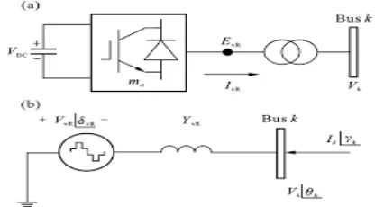
The STATCOM is a FACTS controller based on voltage sourced converter. A VSC generate a synchronous voltage
of fundamental frequency, controllable magnitude and phase angle. If a VSC is shunt-connected to a system via a
coupling transformer as shown in Figure 1.1 the resulting STATCOM can inject or absorb reactive power to or from
the bus to which it is connected and thus regulate the bus voltage magnitude. This STATCOM model is known as
Power Injection Model (PIM) or Voltage Source Model (VSM). Steady state modeling of STATCOM within the
Newton-Raphson method in polar co-ordinates is carried out as follows:
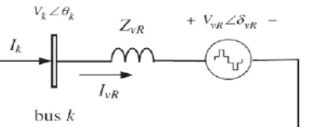
The Thevenin equivalent circuit representing the fundamental frequency operation of the switched-mode voltage
sourced converter and its transformer is shown in Figure 1.2
vR k vR vR
V
=
V
+
Z I
(12)Is expressed in Norton equivalent form
I
vR=
I
N−
Y V
vR vR (13)Where
I
N=
Y V
vR vRIn these expressions,
V
k represents bus k voltage andV
vR represents the voltage source inverter.I
N is theNorton’s current while
I
vR is the inverter’s current. Also,Z
vR andY
vR are the transformer’s impedance andshort-circuit admittance respectively.
293 Figure 1.2 STATCOM equivalent circuit
The STATCOM voltage injection
V
vRbound constraint is as follows:min max
vR vR vR
V
≤
V
≤
V
(14)Where
V
vRmin andV
vRmaxare the STATCOM’s minimum and maximum voltages.The current expression in is transformed into a power expression by the VSC and power injection into bus
k
as shown in equations (15) and (16) respectively.* 2 * * *
vR vR vR vR vR vR vR k
S
=
V I
=
V Y
−
V Y V
(15)* * * 2 *
k k vR vR vR k k vR
S
=
V I
=
V Y V
−
V Y
(16)Where
V
vR andδ
vR are the STATCOM voltage magnitude and angle respectively.The active and reactive power equations for the STATCOM and bus k, respectively:
)],
sin(
)
cos(
[
2 k vR vR k vR vR k vR vR vRvR
V
G
V
V
G
B
P
=
+
δ
−
θ
+
δ
−
θ
(17))]
cos(
)
sin(
[
2 k vR vR k vR vR k vR vR vRvR
V
B
V
V
G
B
Q
=
−
+
δ
−
θ
−
δ
−
θ
(18))],
sin(
)
cos(
[
2 vR k vR vR k vR vR k vR kk
V
G
V
V
G
B
P
=
+
θ
−
δ
+
θ
−
δ
(19))]
cos(
)
sin(
[
2 vR k vR vR k vR vR k vR kk
V
B
V
V
G
B
Q
=
−
+
θ
−
δ
−
θ
−
δ
(20)Using these power equations, the linearized STATCOM model is included in the load flow solution, where the
voltage magnitude
V
vR and phase angleδ
vR are taken to be the state variables.4 Algorithm of AHP Method
AHP is a decision-making tool, which helps in finding goals or objectives among alternative. It is a systematic
method for comparing a list of objectives and the alternative solutions satisfying respective objectives. Some
mathematical steps involved in AHP method are as follows.
Step 1: selection and evaluation of attributes Step 2: selection of alternatives
www.ijiset.com
294
The entire MADM problem can be easily expressed in matrix format. A decision matrix A is an (M × N) matrix in which element aij indicates the performance of alternative Ai when it is evaluated in terms of decision criterion Cj,
(for i = 1,2,3,..., M, and j = 1,2,3,..., N). This decision matrix is taken as an input to all the MADM methods.
Criteria
U
Alternatives C1 C2 C3 … CURUN
AR1R aR11R aR12R aR13R … aR1N
AR2R aR21 RaR 22 RaR 23 R… aR 2N
AR3R aR31R aR 32R aR 33R … aR 3N
.. . . . … .
.. . . . … .
.. . . . … .
ARMR aR M1 RaR M2 RaR M3 R… aR MN R(21)
Step 4: construction of pair wise comparison matrix
The number of comparison is the combination of a number of attributes to be compared. The number of pair wise
comparisons is shown in Table 1.1
Table 1.1 Number of comparisons
Number of elements 1 2 3 4 5 6 7 𝑛𝑛
Number of comparison 0 1 3 6 10 15 21 𝑛𝑛(𝑛𝑛 − 1)
2
The scaling is not necessary 1 to 9 but for qualitative data such as preference, ranking and subjective opinions, it is
suggested to use scale 1 to 9. The values of the pair wise comparisons in the MADM methods are determined
according to the scale introduced by Saaty (1980). According to the scale, the available values for the pair wise
comparisons are members of the set: {9, 8, 7, 6, 5, 4, 3, 2, 1, 1/2, 1/3, 1/4, 1/5, 1/6, 1/7, 1/8, 1/9} and is shown in
Table 1.2
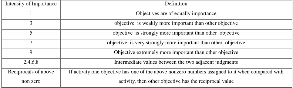
Table 1.2
Scale of Relative Importance (according to Saaty (1980))
Intensity of Importance Definition
1 Objectives are of equally importance
3 objective is weakly more important than other objective
5 objective is strongly more important than other objective
7 objective is very strongly more important than other objective
9 Objective extremely more important than other objective
2,4,6,8 Intermediate values between the two adjacent judgments
Reciprocals of above
non zero
If activity one objective has one of the above nonzero numbers assigned to it when compared with
activity, then other objective has the reciprocal value
For ‘N’ number of objectives, the size of the comparison matrix is N xN. The diagonal elements of the matrix are
always 1 and the upper diagonal has to fill based on preference values using the following rules:
1. If the judgment value is on the right side of 1, put the actual judgment value.
2. If the judgment value is on the left side of 1, put the reciprocal value.
295
1
ji ij
b
b
=
(22)Thus this is complete comparison matrix. All the elements in the comparison matrix are positive or 𝑏𝑏𝑗𝑖>0. The pair wise comparison matrix of objectives is shown in Table 1.2.
U
obj1 obj2 obj3 … objN Priority
obj1 b11 b12 … b1N p1
obj2 b21 b22 … b2N p2
. . . … . .
. . . … . .
U
objN bN1 bn2 … bNN Pn U(23)
Step 5: Find the relative normalized weight
Find the relative normalized weight (
W
j,j
=
1, 2, 3,...
N
) of each attribute by (i) calculating geometric mean ofthe
i
th row and (ii) normalizing the geometric means of rows in the comparison matrix. This can be represented as1
M M
j ij j
GM
=
b
∏
(24)1
j j M
j j
GM
W
GM
=
=
∑
(25)The geometric mean method of MADM methods is commonly used to determine the relative normalized weights of
the attributes, because of its simplicity, easy determination of the maximum Eigen value, and reduction in
inconsistency of the judgments.
Later steps involved in the four methods are
Step6: Calculate matrices
A
3
andA
4
such thatA
3
=
A
1* 2
A
andA
4
=
A
3 / 2
A
, whereA
1
is pair wisecomparison matrix,
A
2
=
(
W W W
1,
2,
3...
W
j)
T.Step7: Determine the maximum Eigen value
λ
max that is the average of matrixA
4.Step8: Calculate the consistency index ( max )
1
MCI
M
λ −
=
−
. The smaller the value ofCI
, the smaller is thedeviation from the consistency.
Table 1.3
RCI values for different values of N
N 1 2 3 4 5 6 7 8 9 10
RCI 0 0 0.58 0.89 1.12 1.24 1.32 1.41 1.45 1.49
www.ijiset.com
296
Step11: The overall performance score of the alternatives is obtained by multiplying the relative normalized weight (
W
j) of each attribute with its corresponding normalized weight value for each alternative and summing over theattributes for each alternative
.
5 Teaching Learning Based Optimization
The demonstration or working of TLBO Algorithm is divided into two parts:
• ‘Teacher phase’.
• ‘Learner phase’.
The first part consists of the “Teacher Phase” and the second part consists of the “Learner Phase”. The “Teacher
Phase” means learning from the teacher and the “Learner Phase” means learning through the interaction between
learners. TLBO searches for the global optimum mainly through two steps: teacher phase and learner phase.
5.1 Teacher Phase
It is the first part of the algorithm where learners learn through the teacher. During this phase, a teacher
tries to increase the mean result of the class in the subject taught by him or her depending on his or her capability. At
any iteration i, assume that there are ‘m’ number of subjects (i.e., design variables), ‘n’ number of learners (i.e.,
population size, k=1,2,…,n) and 𝑀𝑀𝑗,𝑖 be the mean result of the learners in a particular subject ‘j’ (j=1,2,….,m). The best overall result 𝑋𝑋𝑡𝑜𝑡𝑎𝑙−𝑘𝑏𝑒𝑠𝑡,𝑖 considering all the subjects together obtained in the entire population of learners can be considered as the result of best learner kbest. The difference between the existing mean result of each subject and
the corresponding result of the teacher for each subject is given by,
Difference_𝑚𝑚𝑚𝑚𝑚𝑚𝑛𝑛𝑗,𝑘,𝑖=𝑟𝑟𝑖(𝑋𝑋𝑗,𝑘𝑏𝑒𝑠𝑡,𝑖− 𝑇𝑇𝑇𝑇𝑀𝑀𝑗𝑖) (26) Where, 𝑋𝑋𝑗,𝑘𝑏𝑒𝑠𝑡,𝑖 is the result of the best learner in subject j. TF is the teaching factor which decides the value of mean to be changed, and TF is the random number in the range [0,1]. Value of TF can be either 1 or 2. The value of
TF is decided randomly with equal probability as,
TF = round [l + rand (0,1){2-1}] (27)
TF is not a parameter of the TLBO algorithm. The value of TF is not given as an input to the algorithm and its value
is randomly decided by the algorithm using Eq. (27). After conducting a number of experiments on many benchmark
functions it is conducted that the algorithm performs better if the value of TF is between 1 and 2. However, the
algorithm is found to perform much better if the value of TF is either 1 or 2 and hence to simplify the algorithm, the
teaching factor is suggested to take either 1 or 2 depending on the rounding up criteria given by Eq. (27). Based on
the Difference_𝑚𝑚𝑚𝑚𝑚𝑚𝑛𝑛𝑗,𝑘,𝑖, the existing solution is updated in the teacher phase according to the following expression. 𝑋𝑋𝑗,𝑘,𝑖=𝑋𝑋𝑗,𝑘,𝑖+Difference_𝑚𝑚𝑚𝑚𝑚𝑚𝑛𝑛𝑗,𝑘,𝑖 (28) 𝑋𝑋𝑗,𝑘,𝑖 is accepted if it gives better function value. All the accepted function values at the end of the teacher phase are maintained and these values become the input to the learner phase. The learner phase depends upon the teacher
297
5.2 Learner Phase
It is the second part of the algorithm where learners increase their knowledge by interacting among themselves. A
learner interacts randomly with other learners for enhancing his or her knowledge. The random inter-action among
learners improves his or her knowledge. In this stage a teacher choose a student randomly and tries to enhance his
information and knowledge by means of interaction. A teacher reinforces his knowledge by interaction. A learner
learns new things if the other learner has more knowledge than him or her. Considering a population size of ‘n’, the
learning phenomenon of this phase is explained below. Randomly select two learners P and Q such that 𝑋𝑋𝑡𝑜𝑡𝑎𝑙−𝑃,𝑖′
≠ 𝑋𝑋𝑡𝑜𝑡𝑎𝑙−𝑄,𝑖′ (where, 𝑋𝑋𝑡𝑜𝑡𝑎𝑙−𝑃,𝑖′ and 𝑋𝑋𝑡𝑜𝑡𝑎𝑙−𝑄,𝑖′ are the updated function values of 𝑋𝑋𝑡𝑜𝑡𝑎𝑙−𝑃,𝑖′ and 𝑋𝑋𝑡𝑜𝑡𝑎𝑙−𝑄,𝑖′ are the
updated function values of 𝑋𝑋𝑡𝑜𝑡𝑎𝑙−𝑃,𝑖′ and 𝑋𝑋𝑡𝑜𝑡𝑎𝑙−𝑄,𝑖′ of P and Q, respectively, at the end of teacher phase). Teaching-learning -based optimization (TLBO) is a population-based algorithm which simulates the teaching-Teaching-learning process
of the classroom. This algorithm requires only the common control parameters such as the population size and the
number of generations and does not require any algorithm- specific control parameters.
𝑋𝑋𝑗,𝑃,𝑖" = 𝑋𝑋𝑗,𝑃,𝑖′ + 𝑟𝑟𝑖�𝑋𝑋𝑗,𝑃,𝑖′ − 𝑋𝑋𝑗,𝑄,𝑖′ �, 𝐼𝐼𝐼𝐼 𝑋𝑋𝑡𝑜𝑡𝑎𝑙′ − 𝑃𝑃, 𝑖𝑖 < 𝑋𝑋𝑡𝑜𝑡𝑎𝑙−𝑄,𝑖′ (29)
𝑋𝑋𝑗,𝑃,𝑖" = 𝑋𝑋𝑗,𝑃,𝑖′ + 𝑟𝑟𝑖�𝑋𝑋𝑗,𝑄,𝑖′ − 𝑋𝑋𝑗,𝑃,𝑖′ �, 𝐼𝐼𝐼𝐼 𝑋𝑋𝑡𝑜𝑡𝑎𝑙′ − 𝑄𝑄, 𝑖𝑖 < 𝑋𝑋𝑡𝑜𝑡𝑎𝑙−𝑃,𝑖′ (30)
5.3 FLOWCHART OF TEACHING LEARNING BASED OPTIMIZATION
www.ijiset.com
298
6 Results and Discussion
6.1. IEEE 30-bus system results
This section presents the details of the study carried out on IEEE 30-bus system for power system performance
enhancement. The maximum and minimum values for the generator voltage and tap changing transformer control
variables are 1.1 and 0.9 in per unit respectively. The maximum and minimum voltages for the load buses are
considered to be 1.05 and 0.95 in per unit. The case studies for simulation study are as follows:
Case I: Single-objective optimization with STATCOM device at the selected locations. Case II: Application of MADM methods for determination of optimal location of STATCOM Case I: Single-objective optimization with STATCOM device at the selected locations
In the present power system operation, the utilities need to operate their power transmission system much more
effectively, increasing their utilization degree. Reducing the effective reactance of lines by series compensation is a
direct approach to increase transmission capability. However, power transfer capability of long transmission lines is
limited by stability considerations. Because of the power electronic switching capabilities in terms of control and
299
performance of the power system. The proposed TLBO algorithm is applied for solving the optimal power flow
problems subjected to different equality and inequality constraints with STATCOM device in the selected locations.
The selected locations of STATCOM are at buses 9,10,12,14 and 16. These locations are taken based on first five
maximum voltage deviations of load buses from steady state values of load buses. The TLBO algorithm is applied
for solving the OPF problem with four different objective functions. In each case study, four sets of 10 test runs were
performed for solving the OPF problems under three operating conditions. All the solution satisfies the constraints
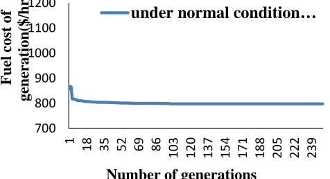
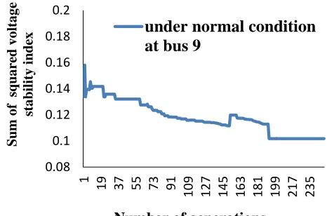
on reactive power generation limits and line flow limits. Figures 1.3(a)-1.3(d) shows the convergence characteristics
of fuel cost of generation, total real power loss, sum of squared voltage stability index and voltage deviation with
STATCOM located at different locations of optimal value under three operating conditions. From these figures it can
be observed that the TLBO algorithm reaches the best solution within 150 iterations under all the operating
conditions. Table 1.4 shows the OPF results with STATCOM device located in the selected lines with respect to
different objective functions. Table 1.4 shows four different attributes (objectives) such as total fuel cost of
generation, total real power loss, sum of squared voltage stability index and voltage deviation with five different
alternatives (different lines)such as 9,10,12,14 and 16 buses has being taken for STATCOM device installation.
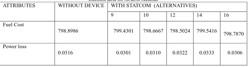
Also from the Table 1.4, it can be observed that under normal condition the optimal value for cost of generation is
798.5024 $/hr at bus 12, the optimal value for power loss is 0.0306 p.u at bus 9, the optimal value for voltage
stability index is 0.1018 at bus 9 and optimal value for voltage deviation is 0.0007 at buses 10 and 12. With this one
can say that optimal values of four attributes are obtained at different alternatives.
Case II: Application of MADM methods for determination of optimal location of STATCOM
In this section, in order to differentiate the best alternative out of five considered alternatives 9,10,12,14 and 16
MADM method is applied. The decision making method considered for determination of best location of
STATCOM is AHP. The same preference matrix given in Table 1.5 is also considered here. This matrix is based on
the preferences given to the four attributes i.e. the pair wise comparisons determines the preference of each attribute
over another. Table 1.6 also used as priority vector of the attributes. Priority vector shows relative weights among
the attributes that are used for comparison. Table 1.4gives the OPF results with STATCOM device located at buses
with respect to different objective functions and are used as decision table for MADM methods. The considered
decision matrix of MADM methods for the system consists of 5 alternatives (different buses)such as 9,10,12,14 and
16, 4 attributes(objectives) such as total fuel cost of generation, total real power loss, sum of squared voltage
stability index and voltage deviation. This decision matrix is given as an input to all the methods. The element in this
matrix indicates the performance of alternative when it is evaluated in terms of decision criterion.
Table 1.4
Decision table for MADM Methods
ATTRIBUTES WITHOUT DEVICE WITH STATCOM (ALTERNATIVES)
9 10 12 14 16
Fuel Cost
798.8986 799.4301 798.6667 798.5024 799.5416
798.7870
Power loss
www.ijiset.com
300 Voltage stability index
0.1057 0.1018 0.1034 0.1029 0.1037 0.1044
Voltage deviation
0.0008 0.0008 0.0007 0.0007 0.0009 0.0008
Table 1.5
Pair Wise Comparison Matrix for Attributes
Attributes
Attributes
Fuel Cost
Power Loss
Voltage Stability
Index
Voltage Deviation
Fuel Cost Power Loss Voltage stability index Voltage deviation
1 1/2 1/3 1/3
2 1 1/3 1/5
3 3 1 1/2
3 5 2 1
Table 1.6
Weight Matrix and value of attributes
Attributes Weight-age Subjective measure of attribute
Assigned Value
Fuel Cost Power
loss Voltage stability index Voltage deviation
0.4266 0.3427 0.1422 0.0885
Eigen value Consistency
index Consistency
ratio
4.1548 0.0516 0.0580
Table 1.7
Relative Ranking of Alternatives under different operating conditions MADM methods
Alternatives AHP
9 2
10 1
12 5
14 3
301
Table 1.7 shows that relative ranking of alternatives under different operations by MADM methods. From the Table
1.7 it is observed that AHP method gives rank one for alternative 10. From this it is can say that AHP method gives
rank one to the alternative 10 for the STATCOM location and so it is considered as a best choice for the location of
STATCOM device among the buses considered for the system and this gives highest benefits to the power system
operation in terms of performance parameters. Figure 1.4(a)-1.4(d) shows the convergence characteristics of fuel
cost of generation, total real power loss, sum of squared voltage stability index and voltage deviation with
STATCOM located at optimal bus 10. Tables 1.4(a)-1.4(b) shows that the optimal control variables settings for OPF
without and with STATCOM device located at the optimal bus10. From figure 1.4(a)-1.4(d), it is observed that the
convergence characteristics of the four objectives obtained are better when compared to without STATCOM device
and at optimal location 10 STATCOM gives better performance compared to other locations.
Figure 1.3(a) Convergence of fuel cost of generation
Figure 1.3(b) Convergence of total power loss 700 800 900 1000 1100 1200
1 18 35 52 69 86 103
12 0 13 7 15 4 17 1 18 8 20 5 22 2 23 9
F
u
el
co
st
o
f
ge
n
er
at
ion
($/
h
r)
Number of generations
under normal condition…
0 0.05 0.1 0.15 0.2 0.25
1 18 35 52 69 86 103
12 0 13 7 15 4 17 1 18 8 20 5 22 2 23 9
T
ot
al
r
eal
p
ow
er
l
os
s (
p
.u
)
Number of generations
www.ijiset.com
302
Figure 1.3(c) Convergence of voltage stability index
Figure 1.3(d) Convergence of voltage deviation
Figure 1.4 (a) Convergence of fuel cost of generation of IEEE30 bus system with optimal location of STATCOM 0.08 0.1 0.12 0.14 0.16 0.18 0.2
1 19 37 55 73 91 109
12 7 14 5 16 3 18 1 19 9 21 7 23 5 S u m of sq u ar ed vol tage st a b ilit y in d ex
Number of generations
under normal condition
at bus 9
0 0.01 0.02 0.03 0.04 0.05 0.06 0.07
1 17 33 49 65 81 97
11 3 12 9 14 5 16 1 17 7 19 3 20 9 22 5 24 1
V
ol
tage
d
evi
at
ion
Number of generations
under normal condition at buses…
750 850 950 1050 1150
1 17 33 49 65 81 97
11 3 12 9 14 5 16 1 17 7 19 3 20 9 22 5 24 1
F
u
el
co
st
o
f g
en
era
ti
o
n
($
/hr
)
Number of generations
303 Figure 1.4(b) Convergence of power loss of IEEE 30-bus system with optimal location of STATCOM
Figure 1.4(c) Convergence of voltage stability index of IEEE 30-bus system with optimal location of STATCOM
Figure 1.4(d) Convergence of voltage deviation of IEEE 30-bus system with optimal location of STATCOM
7. CONCLUSION
In this paper, the TLBO has been successfully performed to solve optimal placement of STATCOM for reducing the
active power loss, enhancing voltage stability index, improvement in voltage deviations and reducing the cost. The
results obtained from the TLBO approach were compared to those reported in the recent literature. It has been
observed here, that TLBO has the efficiency to reduce the active power loss reasonably without violating any
0 0.05 0.1 0.15 0.2 0.25 0.3
1 16 31 46 61 76 91
10 6 12 1 13 6 15 1 16 6 18 1 19 6 21 1 22 6 24 1
T
o
ta
l
rea
l p
o
w
er l
o
ss
(p.
u)
Number of generations
without device under normal…
0.05 0.1 0.15 0.2 0.25 0.3
1 19 37 55 73 91
10 9 12 7 14 5 16 3 18 1 19 9 21 7 23 5
S
u
m
of
s
q
u
ar
ed
vol
tage
st
a
tb
ilit
y
in
d
ex
Number of generations
without device under normal…
0 0.01 0.02 0.03 0.04 0.05 0.06 0.07 0.08 0.090.1
1 19 37 55 73 91
10 9 12 7 14 5 16 3 18 1 19 9 21 7 23 5
V
ol
tage
d
evi
at
ion
s
Number of generations
www.ijiset.com
304
constraints. Moreover, TLBO owns excellent convergence characteristics.Therefore .from the simulation results it
may be concluded that TLBO is superior to the other algorithms. Simulation results for IEEE 30 bus system are
analyzed and graphs are generated for the optimal placement of STATCOM in the transmission line using TLBO
optimization technique based on the AHP method. Graphs are generated for convergence for cost of generator,
power loss, and voltage stability index (VSI) and voltage deviation with and without STATCOM FACTS device.
8. REFERENCES
1)H. Happ. "Optimal Power Dispatch - A Comprehensive Survey," IEEE Transactions on Power Apparatus and
Systems, Vol. PAS-96 (3). pp. 841-854, MaylJune, 1977.
2) J. Carpentier, Optimal Power Flow, Electric Power and Energy Systems, Vol. 1. No. 1, April 1979, pp. 3-15.
3) Alok Kumar Mohanty, Amar Kumar Barik, “Power system stability improvement using FACTS Devices”,
International Journal of Modern Engineering Research (IJMER) Vol.1, Issue.2, pp-666-672 ISSN:
2249-6645.pp.-666-672
4) Ranjit Kumar Bindal, “A Review of Benefits of FACTS Devices in Power System”, International Journal of
Engineering and Advanced Technology (IJEAT) ISSN: 2249 – 8958, Volume-3, Issue-4, April 2014. pp. -105-108.
5) Narain G, Hingorani, Laszlo Gyugyi, “Understanding FACTS: Concepts and Technology of FACTS”, IEEE
Power Engineering Society
6) I. Khan, M. A. Mallick, M. Rafi and M. S. Mizra, "Optimal placement of FACTS Controller scheme for
enhancement of power system security in Indian scenario," Journal of Electrical Systems and Information
Technology, vol. 1, no. 2, pp. 161-171, 2015.
7) P.S. Sensarma, K.R. Padiyar and V. Ramanarayanan, "Analysis and performanc Evaluation of a distribution
STATCOM for compensating voltage fluctuations", IEEE Transactions on Power Delivery, Vol. 16, pp. 259-264,
April, 2001
8) R. Venkata Rao* Review of applications of TLBO algorithm and a tutorial for beginners To solve the
unconstrained and constrained optimization problems
9) Amiri, B. (2012). Application of teaching-learning-based optimization algorithm on Cluster analysis. Journal of
Basic Applied Science Research, 2(11), 11795-11802.
10). Babu, B.S., & Palaniswami, S. (2015). Teaching learning based algorithm for OPF with DC link placement
305
11) Khaled N. Nusair and Muwaffaq I. Alomoush Optimal Reactive Power Dispatch Using Teaching Learning
Based Optimization Algorithm with Consideration of FACTS Device “STATCOM”
12) K.Padma, and Yeshitela Shiferaw Performance Study of the System with optimal location of SVC device using
AHP method under different operating conditions
13) P. Ramesh, K. Padma Optimal Allocation of TCSC Device Based on Particle Swarm Optimization Algorithm
14) K. Padma Comparative Analysis Of Performance Of Shunt Facts Devices Using Pso Based Optimal Power Flow
Solutions
15) K Padma, K Vaisakh Application of AHP method for optimal location of SSSC device under different operating