Inspection interval for maximum future reliability using the delay time model

..

VICTORIA UNIVERSITY

OF TECHNOLOGY

DEPARTMENT OF

MATHEMATICS, COMPUTING

AND OPERATIONS RESEARCH

INSPECTION INTERVAL FOR MAXIMUM FUTURE

RELIABILITY USING TIIE DELAY TIME MODEL

Peter Cerone

(4EQRM3)

September 1990

TECHNICAL REPORT

DEPT OF MCOR

FOOTSCRAY INSTITUTE OF TECHNOLOGY VICTORIA UNIVERSITY OF TECHNOLOGY BALLARAT ROAD (P 0 BOX 64), FOOTSCRAY

VICTORIA, AUSTRALIA 3011 TELEPHONE (03) 688-4249/4225

INSPECTION INTERVAL FOR MAXIMUM FUTURE

RELIABILITY USING 1HE DELAY TIME MODEL

Peter Cerone

(4EQRM3)

September 1990

INSPECTION INTERVAL FOR MAXIMUM FUTURE

RELIABILITY USING

TIIE

DELAY TIME MODEL

P. CERONE

Footscray Institute ofTechnolo2y. Melbourne. Australia. 3011

Abstract

The main problem addressed in this article is the determination of an inspection

interval T max' given the number of inspections m -1, which will result in the maximum reliability at some future point in time t = t

* .

The reliability model developed by Christer

is used in which the notion of delay time is involved, representing the start to eventual

failure of an item subject to a fault detectable on inspection. A numerical procedure is used to solve the model for general delay time density f(h) and time to failure from new density

g(y).

T

max is shown to migrate towards the left hand side of the

interv~

[.

i_ .

.i_]

as , m m-1

the number of inspections increase. If both densities are exponential then the optimal

•

. . . al' h beT t

mspectton mterv 1s s own to max

=iii.

Keywords:

Running Title:

Inspection, Reliability, Decision, Optimisation.

-2-1.

INfRODUCTION

Christer (1987) developed an expression for the reliability of a single component

unit which is subject to a detectable fault. He utilises the notion of delay time which is the

span of time from when a defect is first detectable upon inspection to when it is considered

to have failed. If a defect is found at an inspection then the component is replaced or

repaired to an as new condition and thus avoiding a failure. Inspections

are

assumed to be

non-detrimental. The delay time h is governed by the probability density function f(h).

The probability that a new component at time t =

0

has not failed by time t as a result of a

defect at time y from new is subject to a probability density function g (y) . Both

densities have been obtained experimentally and applied successfully by Christer and

Waller (1984 a, b).

The reliability RT (t) due to a periodic inspection every

T

time units is derived by

Christer (1987) to be

where,

R,-(t) =

r~m)(t)

(m-1) TS t S mT

m-1

r~m)(t)

=

L

~(T) r~m-J)

(t-jT)

+

BT(t)

j=l

with,

and M(x) =

-3-Jl

l)(T) =

J

g(y)M(jT-y)dy,

(j-1 )T

00 t

BT(t) =

J

g(y)dy +

J

g(y)M(t-y)dy

l (m-l)T

00

J

f(h)dh= 1-F(x).

x

(2)

It should be noted that m is a positive integer and throughout the paper the

convention is used that when m = 1 the sum in equation (1), and similar expressions, is

zero.

The main problem to be addressed here is to determine, for fixed number of

inspections m-1, the optimal inspection interval, T that will result in the maximum

reliability at some future point in time t = t

*.

The type of problem envisaged is that of a

mission starting at t = t* until which time the item may be inspected for a fault.

Alternatively we may investigate the optimal inspection interval for a deteriorating item

whose time of commencement of a mission has been delayed.

2. 1HE CONVERSE PROBLEM

Let us assume that it is advantageous for a deteriorating item to be as reliable as

possible at some future point in time t = t

*.

We can inspect the item at periodic intervals of

length T and the item is either renewed or repaired to an as good as new condition. The

problem we wish to address here is to find the optimal inspection interval T max given a

-4-Thus given

t

=

t •

in

(1)

we obtain

m-1

•

•

=L

_j=l (m-j) • • • t t

x:J.(f)

rT

(t -

JT)

+

BT

(t ) , -

ST S

-1

m m- (3)

where

x:j (T) and BT (t*) are as given in (2).

The problem becomes that of finding for each number of inspections m-1, the optimal

inspection interval, Tover the domain indicated in equation (3).

We notice that as m

•

t

increases then T will decrease since the interval of search is of length

m

(m-1)

and the bounds on Twill become tighter.

dr.(m)(i*)

One way of obtaining the optimal inspection interval T would be to find TdT

and determine where it becomes zero. Further investigation would be needed

to be performed to determine whether this was indeed the point at which the global

•

•

. t T t

ed

maximum over -

S

<

-1

occurr .

m

m-It is much easier and more practical to either evaluate

r~>(i*)

over the interval

[

~

·

~:.]

or else use some interval bisection or refinement of mesh to

find

the

maximum. It is

felt that the most practical method would be to actually plot equation (3)

and thus allowing the user the convenience of deciding on a suitable value ofT since there

-5-3.

A SWPLE EXAMPLE

It is instructive to consider a simple example of the problem. Let us examine the

problem shown in the diagram of Figure 1. We wish to perform only one inspection so

that we need to choose when

this

inspection is to occur given that the maximum reliability

at t

=

t

*

is desired.

From the diagram of Figure 1 it may

be

noticed that the earliest possible time the

•

inspection can

be

made is at T

=

~

in which case another inspection is due at our time of

interest t

*.

The latest the inspection can be made is at our point of interest T

=

t

*

resulting

in no benefit Since the inspections are assumed to

be

benign and perfect

it

follows that

r<;>

(r*)

>

r<?>

(i*) =

r~~)

(i*).

Thus having one inspection is better than having none.

t t

-

₂

We wish to find when the optimal inspection should occur.

Consider equation

(3)

with m

=

2 to give

•

r¥>

(i*)

=

1'i(1)r~>

(i*

-T)

+

BT(t•), ; .

S T St.

(4)

Thus the problem becomes that of determining T such that

r~>

(i*)

is a maximum.

For definitiness we take the densities used by Christer (1987) with the delay time density

f(h)

=

ae

·ah

and

g(y)

as uniformly distributed on [0, 10].

From equations

(1) - (3)

we obtain

-aT

10

a

Ki

(T) =

1 -

e

•

• • -a (t -T) •

10

a

BT (t )

=

(10 -

t )

a.+ 1 -

e

,

t S

10

0

(1) -au

1

'

'

I .I

'

'

_'

T t

*

_{2T t}

Figure 1: Diagram showing R,-(t) for 0 St S 2T and the location oft• allowing for

-6-so that equation ( 4) becomes

•

2 (2) • . - aT aT t •

(lOcx)

rT (t )

=

A+ ex T - (b + ex T) e

-Be ,

°2

ST St S 10

(5)

where

and

•

a= lOcx

+

1 , b

=

a - ext

•

•

- at ..at

A

=

ab

+

e , B

=

ae .

If

we let

y =

(10cx)

2

r~)

ct>

then we obtain from equation (5)

1 dY -aT aT

- dT

=

1 + (b +

cxT-1

)e - Be .

ex

Further, a maximum exists since

•

over the interval of interest namely,

~

s Ts

t

S

10.

•

(6)

Consider specifically the situation when

ex

=

0.5 and

t

=

8 then, 4

S

T

S

8

and, from (5) - (6),

=

To {

1 - 6e-4e

T/2

+

(1

+ T/2)e

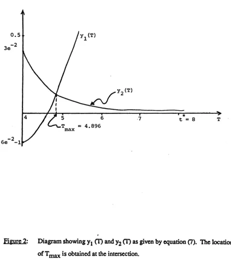
-T/2}.

The critical point is given by the intersection of the curves

-4

T/2 -T/2

y₁

(T)

=

6e e

-landy

₂

(T)=(l+T/2)e

for4STS8.

(7)

The

diagram

in Figure 2 shows a sketch of these curves and their intersection gives

0.5

3e-2

4 6

=

4.896

*

t

=

8 T

Figure 2: Diagram showing

y

_{1 (T)} and

y

_{2 (T)} as given

by

equation (7). The location

-7-Substitution of T max= 4.896 into equation (5) gives (with ex =0.5) the maximum possible

reliability at t* = 8 , given that only one inspection is performed, as ri2> (8) = 0.5124. max

Similarly, r.T<2> (10) = 0.327 where T = 6.637 and we notice that the reliability is

~x mu

lower since it relates to a later time oft*= 10.

4. NUMERICAL SOLUTION OF

rr>(t)

Before proceeding to the solution of the converse problem as represented by equation (3)

we investigate the numerical solution of equation (1) for general densities f (h) and g (y).

Christer (1987] solved equation (1) for f (h) = cxe-cxh and g (y) uniform on (0,10].

We may notice from equation (1) that the evaluation

ofr~m)(t)

at t = (m - 1 + A.)T where

0 SA.

s

1 requires all previous

r~)(t)

fork= (m-1), (m-2), ... , 1 as can be seen from

m-1

r¥11) ( (m-l+A.)T) =

:2,

Kj(T)

r~m-j)

( (m-j-l+A.)T) +BT ( (m-l+A.)T), 0

SA.~

1. (8)

j=l

The ri\t) should be evaluated in the order k = 1, 2, ... , (m-1) since successive terms

depend on all previous tenns. It should further be noted that

A

=

0 represents the

evaluation at the left of an inspection interval and A. = 1 corresponds to the right.

The expression for BT ((m-1

+

A )

1) needed in (8) and given in (2)

may be written in the following form: m-1

BT ( (m-l+A.)T) = 1-

:2,

j=l

JT (m-l+A)T

f

g(y)dy-

f

g(y)F ( (m-l+A.)T-y)dy.

(j-l)T (m-l)T

-8-Thus the numerical evaluation of (8) with (9) involves the evaluation of integrals over an

interval of at most of length T. This gives the ability to control the accuracy of integration.

It may further be observed that A. =

0

corresponding to the evaluation on the left hand side of an

inspection interval, eliminates the second integral tenn in (9) and simplifies the working. This

fact allows for

a

fast determination of the behaviour of the reliability by evaluation at an

inspection point

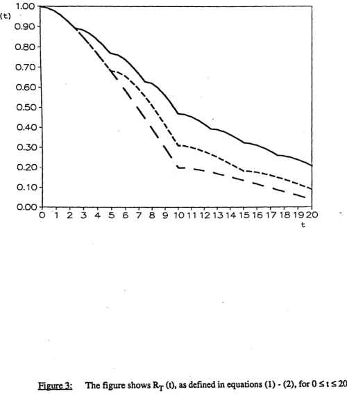
Figures 3, 4 and 5 show the numerical solution of

r~m)(t)

for 0 St S 20 with T = 10, 5

and 2.5 using

a

variety of densities as indicated in the captions. Equispaced points with

A.=

0.5

were taken to produce the.figures however a variable A. to take into account the

behaviour of

r~m)(t)

could possibly be used.

Figure

3

uses the densities f (h) =a e -ah, a= 0.5 and g(y) is uniform on [0,10] for

which

a

closed form expression was obtained by Christer [1987] which has enabled a

comparison with the numerical procedure.

The

behaviourofr~\t)

for (m-l)T St S mT shown in Figures 3-5 may be expected intuitively.

The monotonic behaviour

may

also be shown from the differentiation of equation (1) to

obtain

m-1

r~m)(t)

=

L

~(T) r~M·J\t-jT)

-b,-(t) ' (m-1) St S mT, (10)

j=l

where

t

b.r(t) = -

BT

(t) =

J

g(y) f (t-y) dy .

R.r(t}

0.90

0.80

0.70

0.60

0.50

0.40

0.30

0.20

0.10

'\:,

'

'

,

...

,

'

\

',

'

\

',

_\

\

',

'

\

"'--

...

...

'

"-

--

...

...._

_{...._}

----

--

-

_...

...

...._

0.00+--.--.--r~.---r--r-~-.---.----.~---~~~---'

0 1 2 3 4 5 6 7 8 9 1 0 1 1 1 2 13 14 15 1 6 1 7 1 8 1 9 20

t

Figure 3: The figure shows RT (t), as defined in equations (1) - (2), for 0 St S 20

and T

=

10 ( - -), T =5 (- - -) and T = 2.5 ( _ ). The densities are

0.80

0.70

0.60

0.50

0.40

0.30

0.20 I

~

--

---

-

--

...

---

_{- -==}

--0

.

10

-.::-

-0.00+--,.--.-~--.~.---~-.-~~--~~~~~~---~~

0 1 2 3 4 5 6 7 8 9 1 0 1 1 12 1 3 14 1 5 1 6 1 7 1 8 1 9 20

t

Figure 4: The figure shows RT (t) for 0 St S 20 and

T

= 10 ( - - ),

T

= 5 (- - -) and

1

1.

3 -

2

RT(t)

1.00

0.90

0.80

0.70

0.60

0.50

0.40

0.30

0.20

0.10

O.OQ+--,.---.---.---...--r---.-~-.--.---...-..---.--r--~~--..--.,._.~

0 1 2 3 4 5 6 7 8 9 10 1 1 12 1 3 14 15 16 1 7 18 1 9 20 t

Fieure 5. The graphs depict R,-(t) for _Ost s 20 and T

=

10 ( - - ), T

=

5 (- - -) and T

=

2.5 ( _ _ ). The densities are f(h)

=

0.5 e • O.Sh and

-9-We may deduce from equation (10) that

r~m)(t)

is a continuous monotonically

decreasing function oft with a zero right hand slope at t

=

(m-1) T with possible discontinuities

of derivatives at multiples of T.

We may notice that the graphs in Figure 4 decrease at a faster rate than those in Figure 3

since it takes on average shorter delay time for a fault to become serious enough for action

to be taken on the unit. The delay time density f(h)

in

Figure 4 is Weibull with the shape

parameter~= 1.5

and the characteristic life T\

=

1.0 rather that f (h)

=

0.5e·

0.5h

used to

produce Figure 3. Further, the graphs is Figure 5 also decrease at a faster rate than those in

Figure 3 where the delay time density is the same but g(y)

=

0.25e

-0.25y

rather than uniform on

[0, 10] so that failures are occuring more frequently on average.

5.

SOLUTION OF

THE

GENERAL CONVERSE PROBLEM

Returning now to the solution of equation (3) we note that in order to evaluate

•

•

(m) • t t

rT

(t )

for

'iii

.s

T

<

m-l

we need

r~k)

(t • -

(m - k)T)

fork= l, 2, ... , m-1.

Thus we may use the procedure outlined in the previous section to evaluate.

r~l

(t)

=

~

1)

(T)

r~·J)

(t -jT)

+

B,-(t) (11)

j=l

• . • (m) •

at

t

=

t -

(m-k)T for k

=

1,2, ... m to give rT

(t ).

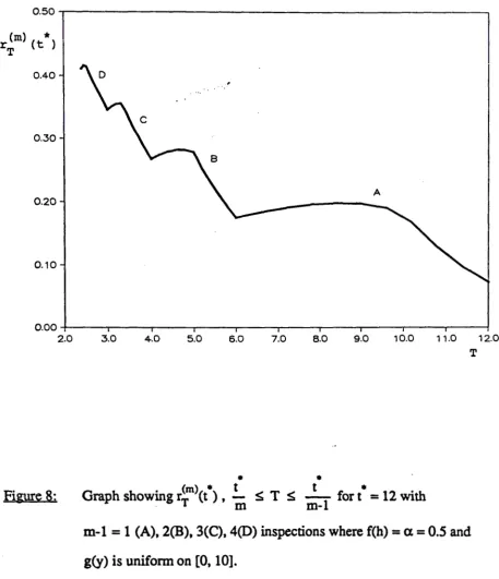
-10-Figure 6 - 8 are based on the exponential delay time density f(h) = cxe-<Xh, ex=

0.5

and

g (y) is uniform on [0, 10]. The three figures show the reliability at t• = 8, 10, 12

respectively with varying inspection interval T for one inspection (A) through to four inspections

(D). The possible range of T clearly depends upon t• and m.

In each of the sections of the

graphs A-D we notice that there is a point T max• depending on the number of inspections, which

results in the maximum reliability at= t•.

There are a number of observations that can be made from Figures 6-8. We may notice

the effect of the uniform density on [0, 10] coming through in Figure 8 in which a defect

exisiting in an original component will lead to a renewal if it has not caused a component failure.

This effect does not manifest itself in either Figure 6 or 7 since t•

<

10.

Further, it is interesting to note that the inspection pericxl Tmax occurs closer to the left of the

interval [

i_,

i__]

the smaller t• is. We may also observe that T migrates towards

m ~1 mu

•

the left hand side of the interval of interest, namely towards

~

, which increasing m. m

This observation begs the question as to how many inspections are needed prior to

4.m)

ct>

being as close as we wish to r<r:>

ci*>.

max t

m

We use two measures Lm and ~ to demonstrate the approach of T max towards

•

t

Lm shows the relative difference between these values and Rm shows

-·

_m

•

the relative effect on the reliability at t=t if the inspection period was taken

•

t

as -

_m

rather than T .

0.65

0.60

0.55

0.50

0.45

0.40

0.35

0.30 +----....---..----,...---~---,.---r----1

1.0

Fi&nre 6:

2.0 3.0 4.0 5.0 6.0 7.0 8.0

T

•

(m) •

t•

t

•

Graph showing r.T (t ) , - S T S

-1 , for t = 8

m

m-with m-1=1(A),2(B), 3(C), 4(0) inspections where f(h) = ae-ah, a= 0.5

0.50

0.45

0.40

0.35

0.30

0.25

0.20

0.15

0.10+-~~-r~~---.,...--~~...--~~-r-~~-.-~~---..~~~~~----l

2.0

Fitmre

7:

3.0 4.0 5.0 6.0 7.0 8.0 9.0 10.0

T

•

•

Graph showing

r~m)(t•),

t ~ T ~ -t •

1 fort = 10 with

m

0.50 . - - - .

0.40

0.30

A

0.20

0.10

0.00 +---.----.---...---.---~----.,----r---r---r----1

2.0

Figure 8:

3.0 4.0 5.0 6.0 7.0 8.0 9.0 10.0 11.0 12.0

T

•

•

(m) • t t •

Graph showing tT (t ) , - S T S - fort

=

12 with

. Ill

Dl-1

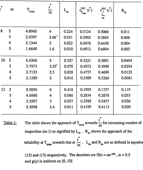
-11-Table 1 shows Lm the ratio of the distance between Tmax and t*/m to the total

length of the interval of observation

D

_m viz

•

Tmax

t

m

L _m

₌

D _m

•

where t

m(m-1) ·

The table also shows

~

=

m

•

demonstrating that the maximum reliability at t = t very quickly approaches from

•

the right T

=

~

the smaller

t

is and the greater the number of inspections m-1.

m

(12)

(13)

Dete~g the value ofTmax is more crucial the larger t• and the fewer number

of inspections required.

It is interesting to observe the effect of inspections on

r~m>

ct)

from Table 1

mu

fort*= 8, 10 and 12. These may be compared with the reliability values of 0.3963, 0.1986

and 0.0731 respectively when no inspection takes place. These values correspond to the

•

t m

8 2

3 4

5

10 2

3 4

5

12 2

3 4 5 Table 1:

-12-•

t

r.(m) (t•) r(~)

ct)

T _max

-

L

_R

m m _{Tmu t} m

-

m

4.8960 4 0.224 0.5124 0.5066 0.011

2.9397 2.66° 0.051 0.5902 0.5865 0.006 2.1344 2 0.022 0.6476 0.6450 0.004 1.6640 1.6 0.010 0.6912 0.6894 0.003

6.6368 5 0.327 0.3221 0.3091 0.0404

3.7973 3.33. _{0.070 0.4072 0.3989} 0.0204 2.7133 2.5 0.028 0.4757 0.4699 0.0122 2.1280 2 0.016 0.5309 0.5266 0.0081

8.5056 6 0.418 0.1995 0.1757 0.119

4.6880 4 0.086 0.2834 0.2678 0.055 3.3507 3 0.037 0.3588 0.3457 0.036 2.5098 2.4 0.011 0.4199 0.4113 0.020

•

The table shows the approach of T . towards

!_

for increasing number of

max

m

inspection (m-1) as signified by

Lm

•

Rm

shows the approach of the

•

reliability at T towards that at

!_ .

L and R are as defined in equations max

m

m m

(12) and (13) respectively. The densities are f(h) = ae-Oh, a= 0.5

-13-It may further be observed from Figures 6 on, that:

(i)

•

•

(ii) rT ( t ) (m) • = r..:.. ( (m) t ) for some -• t ~

T

t

1,

T

2, ~ - ,

i -r2 m m-1

•

•

(iii) r(m:

ct)

<

r~m)

(t.) for some

.!_.

t

m

t

<T<

m-1 '

-

m-1

•

•

(iv) r;m+l\t•)

~

r.T(m) (t•) for some

B

>

0,

!._ -

5

S 't S

!._

- m m m m

The first observation states that if the best possible inspection period is chosen then

increasing the number of inspections improves the reliability. Increasing the number of

inspections in itself, is not reasonably enough to guarantee an improvement in the

reliability as demonstrated by obervation (iv). Point (ii) follows immediately from the fact

that since there is an optimal impection interval

Tmax

then there are points

T

₁ and

T

₂ with

which the reliability at t

*

is equal. This point only holds provided

T

max does not occur at

an end point. (It will be shown subsequently that this situation arises when both densities

are exponential). Observation (iii) results from the fact that the last inspection is made at

0.40 .---~

r <,rn) (t *)

'I: 0.35

0.30

0.25

0.20

A

0.15

0.10

0.05

0.00 ----.---.---..---.---...----~--....---t

2.0 3.0 4.0 5.0 6.0 7.0 8.0 9.0 10.0

T

•

•

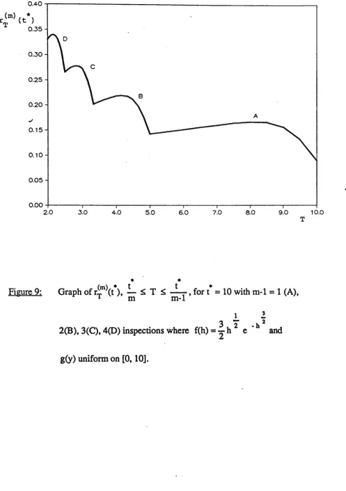
Figure 9: Graph ofr.T (t ), -(m) • t S T S -t •

1 , fort = 10 with m-1=1 (A),

m

m-1

!

3 -

2

2(B), 3(C), 4(0) inspections where f(h)

=

2

h 2

e -h and

-14-We now return to looking at the converse problem corresponding to the densities

used to produce Figures 4 and 5. The future point of interest t•

=

10 is used to produce

Figure 9 demonstrating when compared with Figure 7, the effect of a change to a Weibull

delay time density which has a shortening of the average delay time when compared to the

exponential density with

ex=0.5. The optimal inspection intervals Tmax are further to the right in

[ f .

~:1]

.

•

Figure 10 shows the graph of

r~m)

(t)

for t

m

•

t •

S T S

-1

with t

=10

m-and m

=

2, 3, 4, 5 where

both

densities are exponential. We notice that the optimal

inspection interval occurs at the left hand limit, namely

•

t

(14)

--

_m

.

That is, the maximum reliability is obtained

if

we choose T in such a way that an

inspection is due at our point of interest t

=

t• but is not carried out. This is due to the

memoryless property of the exponential.

It is interesting to demonstrate equation (14) analytically when the densities are both

0.50 .,---~

r(m) (t*) .

T

0.45 _D

0.40 I

0.35

0.30

0.25

0.20

0.15

0. 10 +----r---r----.----,.---...----.----...---1

2.0

Figure 10:

3.0 4.0 5.0 .

•

Graph

ofr~>

(t),

-in

~

T

~

6.0 7.0 8.0 9.0

T

•

t •

-1, fort

=

10 with m-1=1 (A),

m-2(B ), 3(C), 4(0)

inspections

where f(h) = ae-ah, a= 0.5 and g(y)

=

13e-Ph,

p

=

0.25.

-15-6.

CONCLUSION

The paper has addressed the problem of detenning the optimal regular inspection

period for maximum reliability at some future point in time for a given number of

inspections. The general reliability model developed by Christer, which includes the

notion of delay time, has been solved in principle for any two densities of delay time and

time to failure from new. The numerical method used has been further developed to allow

a solution of the converse problem stated above and the approach of

Tmax

towards

t•

/m for

increasing number of inspections m-1 has been demonstrated.

The work may

be

developed to take into account the use of cost models giving a

trade-off between cost of mission failure and inspection cost. Such a cost model may be to

determine m • and

~

such that

K • •

m ,T

min

=

_m,

_T

K _m,T

with

c being the inspection cost and C the cost of mission failure.

(15)

Equation (15) may

be

written in a slightly different form from which a number of

observations may

be

made easily.

Viz,

-16-Firstly, we note that (m-l)c

<

C so that the cost of m-1 inspections is less than the

cost of mission failure making the term in the square brackets negative. This observation

gives us a bound on the number of inspections and so

m-1=I,2, ···{;]. (17)

with [ ; ] meaning the smallest integer part of ; .

A second observation which may be made is that since the term in square brackets in

equation (16) is negative, then for fixed m we have that ~Tis minimal

(m) • • • • (m) • •

where rT (t ) 1s maximal. That 1s at r.T (t ) so that T = T .

mu max

A search through m as given by equation ( 17) into equation (16) with T =

T*

=

T max will give m •. T max does of course change with m even though it is not explicity

shown.

Thus the problem of solving (15) becomes that of finding m • in

~

{ c+[Cm-l)c-C]

r~':<t'>},

m=2,3, ...

[~]

+I. (18)

As a simple example consider the problem with t• =12, c =1 and C = 3.5 then, using

the data in Table 1, m• = 2 and

T*

(corresponding to m=2) = 8.5056. H C=4.5 then,

m*=3 and~= 4.6880.

7. ACKNOWLEDGEMENT

The author wishes to thank Professor A.H. Christer for introducing him to the area

and for the many useful discussions and comments. The work was initiated while on leave

-17-APPENQIX: The Double Exponential Problem

•

We wish to show that

r~m)

(t) is maximal when T

=-in

if both densities are exponential.

Suppose the delay time density to

be

f(h) = ae -Oh and the time to the appearance

of a fault from new to be governed by g(y)

=

~e ·PY then, from (1), (2)

with

and

B ( )

T t - -

_

1 [

cx.e

-

p

t

- ..,e

A. -

a

t

• e

(a-P)

(m-l)T]

.

cx.-f3

. 1

1C(1) =

lCBJ-J

1C

=

1C (T)

= _JL

(B-A]

1

cx.-f3

-aT -~T

A=e

, B=e

.

Now from (3) and (Al) we obtain

•

( 1)

R .. -at (a-~) (m-l)T

- m-

I-""

e

,

•

•

t t

S T S

-m m-1

where u

=

t* - jT.

•

T t .

Evaluation of (A2) at

= -

gtves

m

dr~)

ct> -

~

[lC·. (T) tT(m-j) ({m-j)

~))

- j lC. (T) f.T(m-J) ((m-j) {__)].

dT

£.J

J

m

J

m

.

j=l

R m-1

- (m-1) .., a B

(Al)

(A2)

-18-ex

B -

AA

where a

= ___

..,_

ex-~

' j-1 •

Kj (T) =

~

B [A -

J

x:)

•

and A, B and Kare given in (Al) with T =

!.. .

m

We now notice that to evaluate (A3) we need

•

•

r<!) (

k

!__)

and

r~)

(

k

!__)

for

k

=

1,2, .... , m-l.

t m t m

m m

•

(A4)

To this end putting T =

~

in equation (3) and using (Al) we obtain the recurrence

m

relation

•

Bj-l

u

.

+

a

Bm-l m-J

where

u

=

r<r:>

(m.!._) =

r(~)

(t•).

m t m t

m m

Equation (A5) can be shown to have a solution given by

m

u

_m

=

a

with a= K

+

B from (Al) and (A4).

(A5)

(A6)

Further, differentiating equation (1) with respect tot, using equation (Al) and putting

•

t • .

T = - and t=t weobtam

m

m-1

v

= 1' ~ Bj-l

v

.

- ex

KBm-l

m ~ m-J

which has solution

m-1

v

_m = -

ex Ka

•

with

v

=

r

(~)

(

m.

~)

=

r(~)

(t.) .

m t m t

m m

-19-(A7)

Substitution of (A4), (A6) and (A7) into equation (A3) gives after some algebra

__..!._ (t > =

J3A

L

Bj-l am-j-l [a -j (a-B)] -

(m-1)

Bm-l

dr.(m) • { m-1 }

dT j=l

-o

-

.

dr.(m) • •

Thus __..!._ (t >

=

O when T

=

~

and so is a critical point. It remains to show

dT

m

that it is maximal. To this end, we need to show that

r<~>

ct>

>

r<m}

ct>.

t t

m m-1

Now, from (A6) and using (Al) and (A4) we obtain

(m) • m

r.

(t)

=

a

=

t

m

ex-

J3

(A8)

-20-•

Frth _{u er, usmg equation (3) and (Al) with T} . . _{= -}t _{results in}

m-1

satisfying

which has solution

w = r(m)

m •

t

-

m-1

m-1

Wm= 1C

L

j=l

•

. t

((m-1). - ) m-1

Bj-1 w.+ Bm-1

m-J

m-1

w

_m =a

•

t• t

- a -

-~-with

a

given by (A4) and A = e m-l , B = e m-l

Thus,

(m)

r •

t

m-1

•

(t) =

cx-(3

(AlO)

The inequality given by (A8) can be shown to hold since from equation (A9) and (AlO) we

•

•

have with D =

e -

p

t and C =

e -

at

1 1

-

-cxD

m -

f3

Cm

1 1

-

-a

₀ m-1 _

f3

Cm-1

1 1

-•

t

Hence the maximum occurs when T = - if

both

densities are exponential.

-21-REFERENCES

Birolini, A., (1985),

"On the Use of Stochastic Processes in Modelling Reliability

Problems",

Springer - Verlag.

Christer, A.H., (1987)

"Delay Time Model of Reliability of Equipment Subject to

lmspection Monitoring",

J.

Opl. Res. Soc.

33, 723 - 732.

Christer, A.H., and Waller, W.M., (1984a)

"Reducing Production Downtime Using

Delay Time Analysis"

J.

Op/. Res. Soc.

35, 6, 499 - 512.

Christer, A.H., and Waller, W.M., (1984b),

"An O.R. Approach to Planned Maintenance: