Fully Secure and Succinct Attribute Based Encryption for Circuits
from Multi-linear Maps
Nuttapong Attrapadung AIST, Japan
Abstract
We propose new fully secure attribute based encryption (ABE) systems for polynomial-size circuits in both key-policy and ciphertext-policy flavors. All the previous ABE systems for circuits were proved only selectively secure. Our schemes are based on asymmetric graded encoding systems in composite-order settings. The assumptions consist of the Subgroup Decision assumptions and two assumptions which are similar to Multi-linear Decisional Diffie-Hellman assumption (but more complex) and are proved to hold in the generic graded encoding model. Both of our systems enjoy succinctness: key and ciphertext sizes are proportional to their corresponding circuit and input string sizes. Our ciphertext-policy ABE for circuits is the first to achieve succinctness, and the first that can deal with unbounded-size circuits (even among selectively secure systems). We develop new techniques for proving co-selective security of key-policy ABE for circuits, which is the main ingredient for the dual-system encryption framework that uses computational arguments for enforcing full security.
Keywords. Attribute-based encryption for circuits, Full security, Multi-linear maps, Dual system encryption, Ciphertext-policy, Key-policy, Succinctness
1
Introduction
Attribute-based encryption (ABE), introduced by Sahai and Waters [25], is an important paradigm that generalizes traditional public key encryption. Instead of encrypting to a target recipient, a sender can specify in a more general way about who should be able to view the message. There are two variants of ABE: Key-Policy [18] and Ciphertext-Policy [4]. In a key-policy ABE system, a ciphertext encrypting message M is associated with attribute x. A secret key, which is issued by an authority, is associated with policy f which is a boolean function from some class F. The decryption on a ciphertext associated with xby a secret key associated with f will succeed if and only if f(x) = 1. In a ciphertext-policy ABE system, the roles of f and x are exchanged: they are associated to ciphertext and secret key respectively.
The standard security requirement for ABE is adaptive security which is also dubbed as full security. However, all the available ABE systems for circuits [9, 17, 12] were proved only in a weaker model called selective security. Such a notion requires the adversary to announce a target stringx? upfront before seeing the public key, after then, he can ask for secret keys forf such that
f(x?) = 0. This is in contrast with full security where the adversary receives the public key first and can adaptively ask for secret keys and choose a target string in any order. There is a trivial method to generally bootstrap selective security to full security calledcomplexity leveraging. In this approach, the reduction algorithm would guess which string will be chosen asx? and simulate the security games from it. Hence, the reduction cost to the underlying hard problem will be reduced by factor 2−n, where n is the length of string x, which the probability that the guess is correct. Constructing ABE for circuits with polynomial reductions in all parameters (includingn) to some underlying problems has been an important open problem.
Our Contributions. We propose new fully secure ABE systems for circuits with polynomial reduction (these are the first such schemes, along with concurrent and independent work, see below). We provide both key-policy and ciphertext-policy variants. Both of our ABE systems allow circuits with unbounded size and unbounded fan-out (but bounded depth and bounded input-size), which is exactly the same property as obtained by the KP-ABE of GGHSW [9]. In particular, our CP-ABE is the first scheme (even among selectively-secure ones) that allows unbounded-size circuits. The CP-ABE of GGHSW allows only bounded-size circuits due to their use of universal circuits.
Both of our ABE systems enjoy succinctness, meaning that, for the key-policy variant, the size of a key for circuit f is proportional to the size of circuit f, and the size of a ciphertext for boolean stringxis proportional to the number of 1’s inx. Our CP-ABE system also has analogous efficiency; in particular, to the best of our knowledge, it is the first to achieve succinctness (even among selectively-secure ones). We discuss this in §8.
Our ABE systems are based on multi-linear maps. More precisely, we use composite-order asymmetric graded encoding systems. Such systems was proposed by Coron et al. [7] and was recently extended by Gentryet al.[13] to the composite-order setting. In our schemes for circuits of bounded depth `, we require 3`-multi-linear maps. We introduce some new assumptions on graded encoding: two subgroup decision assumptions which are extended naturally from the case of bilinear maps, and two assumptions which are similar to the Multi-linear Decisional Diffie-Hellman Assumption (MDDH) [6,7]. One of the MDDH-related assumptions is parameterized and quite complex, but we prove that they hold in the generic graded encoding model. The parameters for the assumption depend only on the size and depth of a circuit in one query (and not on the number of key queries). The reduction cost to these assumptions is O(q1) where q1 is the number of pre-challenge key queries (and hence we obtain polynomial reduction as desired).
As another independent work, Waters [31] recently proposed fully-secure functional encryption
(FE) for circuits based on indistinguishability obfuscation (IO) [10,14]. His result is thus stronger than both ours and GGHZ. However, the current security proof of IO under a polynomial-size set of assumptions requires complexity leveraging and hence exponential loss in reduction [14].
1.1 Difficulties and Our Approaches
Applying Dual System Frameworks. Dual system encryption techniques, introduced by Wa-ters [29], have been successful approaches for constructing fully-secure ABE (for simple classes). Our attempt will be to apply this approach to an existing (selectively-secure) KP-ABE for circuits, namely the GGHSW scheme. Until recently, dual system approaches had been considered as se-curity proof “techniques”, where many technical subtle details are buried deep inside the proof, and sometimes this makes it hard to understand. To this end, Wee [32] and Attrapadung [1] in-dependently proposed generic frameworks for dual system approaches. They introduce sufficient primitives (called predicate encoding in [32], and pair encoding in [1]), defined for a predicate, that imply fully-secure ABE for that predicate via generic constructions. Both works describe abstrac-tions of information-theoretic arguments which seem to be essential but were implicit in previous dual-system based schemes. Moreover, the framework of [1] describes also ancomputational analog, which generalizes the technique in the ABE (for boolean formulae) of Lewko and Waters [22].
Difficulties in the Case of ABE for Circuits. We examine our canonical scheme, the GGHSW ABE, using the framework of [1]. It turns out that the underlying structure of GGHSW does not possess information-theoretic security required for the dual-system framework. We believe that an intuitive reason for this can be described as follows. As emphasized by Garg et al.themselves [9], an essential attack that needs to be prevented when considering general circuits is the so-called “backtracking attack”. This attack exploits the distinctive feature of circuits over formulae in that circuits can have gates with fan-out more than one. The attack would occur at an OR gate by somehow “tracking backward”. Therefore, to prevent this was the reason why Garget al.essentially used graded multi-linear maps so that the information can flow only forward (towards the output gate). Now, if we would consider their underlying structure in an information-theoretic sense,i.e.,
without encoding in multi-linear groups, the countermeasure to backtracking will then essentially be lost. Hence, this is the reason why the dual system framework that uses information-theoretic argument would not work for GGHSW. We indeed elaborate checking it concretely in §D.
Applying Computational Approach. The framework of [1] provides a variant of dual system framework that uses computational arguments as ingredients, and was generalized from the ABE for formulae by Lewko and Waters [22]. It was applied to ABE systems in which the information-theoretic structure underlies does not possess required security, such as the ABE for regular lan-guages of Waters [30], the short-ciphertext ABE for formulae of [3], the unbounded ABE for for-mulae of [21, 24]. Fully secure variants of these primitives were then successfully obtained via the framework of [1]. We would like to do the same to ABE for circuits of GGHSW. To work in this framework, it is quite surprising that the requirement is roughly that the considering ABE is both selectively secure and co-selectively secure at the same time. (There is a caveat, see below). Co-selective security is a dual notion to (the more widely-known) selective security. Instead of an-nouncing a target stringx? for ciphertext upfront as in the selective security game, the adversary
A would announce a circuit f upfront, the challenger then gives the public key and a key for f, after that, Athen asks for a challenge ciphertext for any stringx? as long as f(x?) = 0.1 There is a caveat that it is not exactly this requirement of selective and co-selective security of ABE itself,
1
we will actually need the analogous notions but of its underlying pair encoding of ABE. The two analogous notions are called selective and co-selective master-key hiding. Nevertheless, by using techniques similarly to [22, 1], we can convert selective security of ABE to selective master-key hiding of pair encoding almost all the time. It is worth noting that proving co-selective security of KP-ABE is likely to be similar to proving selective security of CP-ABE due to its dual nature. The Missing Piece: Co-selectively Secure KP-ABE for Circuits. The GGHSW KP-ABE is already selectively secure. However, the proof of co-selective security for KP-ABE (of GGHSW or other schemes) or selective security proof of CP-ABE (without using universal circuits) is not known. The main technical novelty in this paper is essentially to prove the co-selective security of (a variant of) the GGHSW KP-ABE. (We will indeed prove the full security of our KP-ABE directly, but the co-selective proof structure is essential).
Difficulties for Constructing Co-selectively Secure KP-ABE for Circuits. The first evi-dence that constructing co-selectively secure KP-ABE for circuits, or somewhat equivalently, selec-tively secure CP-ABE for circuits, can be hard is that the selecselec-tively secure CP-ABE scheme for formulae by Waters [28] is proved under an already more complex assumption than the KP-ABE counterpart [18], namely the Parallel BDHE assumption.2
Our goal is to generalize the selective security proof of Waters’ CP-ABE (or equivalently, we may think of co-selective security of its dual KP-ABE) to the case of general circuits. This poses two main issues. First, the output of a gate can be wired as an input to another gate (we call this a hierarchy issue). Second, and more essentially, the output of a gate (or a circuit input) can be wired as inputs of many gates (this is called multi-fanout). In the Waters’ CP-ABE, these two issues were not problematic since the scheme can be thought of using one big gate (multi-fan-in) that can express a linear secret-sharing scheme.
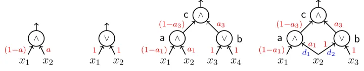
Dealing with Hierarchy. We explain the technical difficulty of this issue via a toy example of circuitf2in Figure1. We would like to apply the simulation for CP-ABE with one gate (e.g.,fAND
in Figure 1) to any gate of f2 in a modular way. In the co-selective proof, the reduction simulates a key for circuit f2 first, gives SKf2,PK to the adversary, and receive a target string x. Suppose that x? = 1100 (so that f2(x?) = 0). The reduction is in the situation where at the AND gate a, the output of ais evaluated to 1 (denoted fa2(x?) = 1). However, if we only use the “stand-alone” proof technique for single gate to this gate a, we will not be able to simulate, since the restriction was that the output of the gate must be 0! We resolve this issue by simulating the key for f2 in such a way that the key elements for lower gates (e.g., gate a) are embedded with all information of the gates (e.g., gate b) that are on their path to the output. Therefore, we effectively chain all the information on the path aggregated to one element. To make the chaining technique work, we have to have a mechanism that identifies gate w such that f2
w(x?) = 0. We do this by providing
“individual randomness” from the assumption to each gate. We elaborate more details in§2.
Dealing with Multi-fan-out. We explain the technical difficulty of this issue via a toy example of circuitf3 in Figure1. The above discussion suggests to simulate a key element atx2 by combining all information from all the paths from it to the output gate,i.e.,both the path throughaand the one throughb. The combined information would cease the “stand-alone” proof technique since the information from each path would interfere the simulation of each other. To solve this, we must distinguish each path; we do this by introducing another set of “individual randomness” from the assumption and dedicate each to each outgoing wire. Another problem that arises when considering multi-fan-out is that we may have many paths from a certain gate to the output gate: it can be exponential size in the depth of circuits. Hence, we cannot afford to have the size of assumption to be as large so as to prepare for any possible chains. We resolve this by decomposing any of possible
Figure 1: Toy Examples: circuitfAND, fOR, f2, f3 respectively. (Texts in colors are related to simulation).
∧
x1 x2 (1−a) a
∨
x1 x2
1 1
∧
c
∧
a ∨ b
x1 x2 x3 x4 (1−a3) a3
(1−a1) a1 1 1
∧
c
∧
a ∨ b
x1 x2 x3
(1−a3) a3
(1−a1) d1
a1
d2 1
1
chains to multiplicative combinations via the use of multi-linear maps in a confined manner so that only required combinations can be produced and no more. We end up with 3`-multi-linear maps for ABE that allows circuits of bounded depth `. We also must find an algorithm for producing the chain information on the fly since the number of all paths can be exponential. We solve this by providing sophisticated recursive algorithms that run in poly-time in the number of gates.
1.2 Other Related Work
Boneh et al. [5] proposed ABE for arithmetic circuits by extending the GVW system. They also proposed KP-ABE for boolean circuits with constant-size ciphertexts. Their systems are selectively secure. Goldwasseret al.[15,16] proposed ABE and FE systems for Turing Machines that are secure against bounded collusions. Our ABE systems are fully secure against unbounded collusions.
2
Toy Examples and Intuition in Technical Details
Before describing formal details, we describe the intuition of our scheme. Readers may skip this in the first read. We illustrate how we solve the difficulties of proving co-selective security of ABE for circuits, mentioned above. We use toy examples for concreteness. We describe these using multi-linear maps in algebraic group setting like in bimulti-linear pairings, which we assume that readers are familiar with. For every system here, we would like prove its co-selective security. In this notion, the adversaryAgives the circuitf that it wants to query, the challenger then gives thePK,SKf to
A, who will then ask for the challenge ciphertext for any stringx of its choice as long asf(x) = 0. In the discussion below, decryption is not important here and we refer to §D.
Toy Example 1: Single-gate Circuit. We first consider a toy ABE system that allows only one gate. Our toy scheme has public keyPK= (gh1
1 , g
h2
1 , e(g1, g2)α), and master keyMSK=α. Keys for
AND,ORareSKAND= (g2α+h1`+h2r, g`2, gr2),SKOR= (g2α+h1`, g
α+h2r
2 , g`2, gr2), resp. (The variable `, r is random and specific to each key). Forx∈ {0,1}∗, letAx ={j|xj = 1}. We define a ciphertext forx∈ {0,1}2 asCT
x= (M e(g1, g2)αs, g1s,{g
shj
1 }j∈Ax). We prove its co-selective security under an assumption stating that given g1, gc11, g
c1a 1 , gz1, g
z a 1, g
zc1 a 1 , g
zc1a
1 , g2, g2c1, g
c2 2 , g
c1a
2 , it is hard to decide if
Z =e(g1, g2)c1c2z or Z ∈RGT. This extends the Bilinear-DH assumption (in asymmetric groups)
with additional elements involving a. The proof is as follows. We consider the case where A chooses to obtainSKAND. The reduction programsα=c1c2,h1 =c1(1−a), h2=c1aby settingPK asgh1
1 =g
c1 1 g
−c1a 1 , g
h2 2 =g
c1a
2 , e(g1, g2)α=e(g
c1 1 , g
c2
2 ). Here, we neglect re-randomizing parameters,
e.g.,definingh2 =c1a+h02for some known randomh02, for simplicity. The reduction then programs
` = −c2, r = −c2 by setting SKAND as g2α+h1`+h2r = g
c1c2−c1(1−a)c2−c1ac2
2 = 1 (when parameters are re-randomized, this implies that it is computable), and g2` = gr2 = g−c2
2 . Simulating in this manner allows us to produce a challenge ciphertext for every case: x= 10 or x= 01. Ifx= 10, we
programss=z(1 + 1a) by setting gs1 =gz1g
z a 1,g
sh1
1 =g1z(1+ 1
a)c1(1−a)=g zc1
a 1 g
−zc1a
mask as Z·e(g
zc1 a 1 , g
c2
2 ). If x= 01, we simply program s=z by setting gs1 =g1z,g
sh2 1 =g
zc1a 1 , and the message mask as Z. An important point here is that in both cases, an unknown critical term
gzc1
1 is canceled out: theg
shj
1 terms only haveg
zc1x
1 for somex6= 1. We may say that (1 +1a) acts as
a “selector” that triggers canceling 1 in (1−a). The case forORis similar but more straightforward as the “coefficients” for the left child and right child become both 1 (that is, h1 =c1, h2=c1).
Toy Example 2: Depth-two Circuit. Next, we show how to deal with hierarchy by considering a toy circuit with depth two. The idea is to construct ABE for this class by using the single-circuit scheme at each gate. We use asymmetric graded 3-linear mapsG1×G2×G3→GT. Letgibe a
gener-ator in each group. Denoteg12=e(g1, g2), and so on. This toy scheme hasPK= (g1h1, . . . , g1h4, g123α ),
MSK=α. For the circuit f2 in Figure1,SKf = (Ka, Kb, Kc) where Ka = (g2αa+h1`a+h2ra, g
`a
2 , g
ra
2 ),
Kb = (g2αb+h3`b, g
αb+h4rb
2 , g
`b
2 , g
rb
2 ), and Kc = (g
α+αa`c+αbrc
23 , g
`c
3 , g
rc
3 ). Note that αw for gate w is randomness dedicated to only this key. We defineCTx= (M g123αs, g1s,{g
shj
1 }j∈Ax). In 3-linear map, the problem instance becomes to to distinguish gzc1c2c3
123 with random. The explanation from §1.1 translates to the following: we will need an information embedded in h1, h2 so that the “selector” at gate c can enable canceling even at the different gate a. We resolve this as follows. First, in order to identify which gate where the selector was chosen, we prepare individual randomnessain the assumption dedicated for every AND gate. (OR gates use coefficient 1). In this example, our assumption would involve a1, a3 (instead of only one a) dedicated to gate a,c, respectively. Then, the reduction programs h1, h2 by “chaining” the information from both gate a and c: it defines
h1 =c1(1−a1)(1−a3) andh2 =c1a1(1−a3). Here, for the left child node, we use (1−a), and for the right child node we usea, as in the first toy example. (We illustrate this with red-colored texts in Fig.1). Moreover, to simulateSKf2, the reduction programs αa=c1c2(1−a3) and`a, ra=−c2,
so that gαa+h1`a+h2ra
2 =g
c1c2(1−a3)−c1c2(1−a1)(1−a3)−c1c2(1−a1)(a3)
2 = 1. Now to simulate CT1100, the
reduction definess=z(1 +a1
3) by settingg
sh1 1 =g
z(1+a1
3)c1(1−a1)(1−a3)
1 . Now, we have canceled out an unknown critical term gzc1
1 by the term (1 +a13)(1−a3). We can afford to put g
zc1x
1 for x6= 1
that is a residue from the “gate mismatch”, e.g., gzc1
a1 a3 1 , g
zc1a1a3
1 in a new assumption, as long as they do not help distinguishgzc1c2c3
123 from random.
Toy Example 3: Fan-out-two Circuit. Next, we show how to deal with multi-fan-out. A key
SKf3 for circuit f3 is exactly the same as SKf2 except that now Kb= (g2αb+h2`b, g2αb+h3rb, g2`b, g2rb). Due to the fan-out two of the second input, the difficulty arises ash2 must contain the “chaining” information forboth paths from it to the output gate. A flawed attempt is to programh2as the sum of both chains: h2 =c1a1(1−a3) +c1·1·a3(1 due tobbeingORgate). However, this would fail the
cancelation when simulating key as: gαa+h1`a+h2ra
2 =g2c1c2(1−a3)−c1c2(1−a1)(1−a3)−c1c2 a1(1−a3)+a3
=
gc1c2a3
2 results in a critical term (since it can be used to break the assumption ase(g
z/a3 1 , g
c1c2a3 2 , g
c3 3 ) =
gzc1c2c3
123 ). We cannot afford modifying αa, h1 altogether to accommodate the path that passes through gateb, since the chaining mechanism would not work anymore. To this end, we introduce a technique so as to distinguish each outgoing wire and makes a mismatch term whenever that wire does not correspond to a gate in consideration. This can be done by preparing individual randomness dedicated for each outgoing wire: in our toy system we used1, d2 for the two wires. We now programh2=c1a1(1−a3)d1+c1a3d2 forPK. Then for gatea, we programra= cd21 and thus set
g2αa+h1`a+h2ra =g2
c1c2(1−a3)−c1c2(1−a1)(1−a3)−c1dc2
1 a1(1−a3)d1+a3d2
=g2
c1c2a3dd2
1. Now we can afford
to put the term occurred from the “outgoing-wire mismatch”,g2c1c2a3 d2
d1, to a new assumption.
First, the chaining mechanism requires terms of formgc1a
e1 1 d1a
e2
2 d2···ae`` d`
1 , one term per one path, to be given in the assumption, where each ai is dedicated to one gate on the path from an input
gate to the output gate,ei ∈ {0,1}, and eachdi is dedicated to one outgoing wire on that path. The problem is that since fan-out can be more than one, the number of possible paths from an input gate to the output gate can be of exponential size in the number of circuit depth (`). Hence, the size of the given terms in the assumption would grow exponentially. We resolve this by using
multi-linearity insideG1also. That is, we defineG1=G01×· · ·×G0`, prepareg10
c1a e1 j1dj1, g0
2
ae2
j2dj2, . . . , g0
` ae`j`dj`
in separate groupsG0i, and let the reduction computes pairing on the fly. This solves the problem of
the assumption size, but then poses another problem that the reduction might run in exponential time due to an exponential number of chains. To this end, we propose a sophisticated polynomial-time recursive algorithm for the reduction to compute chains. See the detail in the proof in§7.3.
Second, the residue from cancellation,e.g.,remaining terms ing1shj from “gate mismatch”, such as g1
zc1a e1 j1a
e2 j2
1 aj3
ae4 j4···ae`j`
, must also be decomposed to groups inside G1 due to the same reason as
above. However, this time if we decompose in a “freedom” manner,e.g., tog01zc1a e1 j1, g0
2
ae2 j2, . . . , g0
` ae`j`
, we would end up having a combination that leads togzc1
1 (by choosing allei = 0), which is a critical term that leads to break the assumption. (We temporarily neglect di terms now for simplicity).
We need to decompose in a restricted way so that all allowed combination must have a1
ji for some
ji. We resolve this by using multi-linearity with one more dimension: G1 =G01× · · · ×G0`+1, and
prepare not only g0iaeiji for alli∈[1, `] but also e(g0
i, g0`+1)
zc1aj1
i for alli∈[1, `]. In this way, to get an element inG1, one must use exactly one element from the latter.
In our ABE, it turns out that we use G1, . . . ,G`+1 for defining the scheme as in [9], and we will decompose G1,G2 respectively to `+ 1 and ` level of multi-linearity for utilizing the assumption. Hence, we will use 3`level of multi-linearity in total. (Due to lengthy discussions here, we postpone one more technique to §D).
3
Definitions
Circuit Notation. A circuit consists of six tuplesf = (`, n,{mi}i∈[2,`],L,R,GateType). We first note that it is wlog that we consider only monotone and layered circuits. (We refer to [9] for the discussion). We let ` be the number of layers, n be the number of inputs, and mi be the number of gates in the i-th layer for i∈ [2, `]. We also define m1 = n for notational consistency. We define Inputs ={w1,1, . . . , w1,n}, and for i ∈[2, `], Gatesi ={wi,1, . . . , wi,mi}. We let Gates =
S
i∈[2,n]Gatesi, and letNodes=Inputs∪Gates. Since we consider only one output gate, we have that
m` = 1, and thatw`,1 is the output gate, which we also denote it aswtop. We defineDepth(wi,j) =i
and Num(wi,j) =j. Since we consider a layered circuit, each of the two inputs of gates in Gatesi
is wired from the output of gates in Gatesi−1. The two functions L:Gates→ Gatesr{wtop} and R:Gates→ Gatesr{wtop} identify those two gates; that is, L(wi,j), R(wi,j) have outputs wired
to wi,j as the first input (left input) and the second input (right input), respectively. We require
that Num(L(wi,j))<Num(R(wi,j)). We note that Depth(L(wi,j)) =Depth(R(wi,j)) =i−1. The functionGateType :Gates→ {OR,AND} specifies the type of gate as eitherOR orAND gate. We also defineGatesORas the set of allORgates, and similarly for GatesAND. We abuse notation and denotef(x) as the output of circuitf evaluated with input stringx. Forw∈Gates, we also denote
fw(x) to be the evaluation of stringx at the output of gate w.
ABE for Circuits: Syntax. Consider a circuit familyFn,` that consists of all circuits with input
• Setup(1λ, n, `)→(PK,MSK): takes as input a security parameter 1λ, the lengthnof input strings to circuits, and the bound ` on the circuit depth, and outputs a public key PK and a master secret keyMSK.
• Encrypt(PK, x, M)→CT: takes as input the public keyPK, a stringx ∈ {0,1}n, and a message M ∈ {0,1}λ. It outputs a ciphertextCT.
• KeyGen(MSK, f) → SK: takes as input the master keyMSK and a circuit description f ∈Fn,`.
It outputs a secret key SK.
• Decrypt(CT,SK)→ M: takes as input a ciphertext CT and the decryption key SK. It attempts to decrypt and outputs a messageM if successful; otherwise, it outputs a special symbol⊥.
Correctness. Consider all messagesM ∈ {0,1}λ, stringx∈ {0,1}n, and circuitf ∈
Fn,` such that f(x) = 1. If Encrypt(PK, x, M) → CTand KeyGen(MSK, f) → SK where (PK,MSK) is generated from Setup(1λ, n, `), thenDecrypt(CT,SK)→M.
Security Notion. An attribute based encryption scheme for circuits is fully secure if no prob-abilistic polynomial time (PPT) adversary Ahas non-negligible advantage in the following game between A and the challenger C. For our purpose of modifying games in next sections, we write some texts in the boxes. Let q1, q2 be the numbers of queries in Phase 1,2, respectively.
1 Setup: C runs(0) Setup(1λ, n, `)→(PK,MSK) and hands the public key PK toA.
2 Phase 1:Amakes aj-th key query for a circuitf(j)∈Fn,`. Creturns(1) SKj ←KeyGen(MSK, f(j)) .
3 Challenge: Asubmits equal-length messages M0, M1 and a target string x? ∈ {0,1}n with the restriction that f(j)(x?) = 0 for allj ∈[1, q1]. Cflips a bit b
$
← {0,1} and returns the challenge ciphertext (2) CT?←Encrypt(PK, x?, Mb) .
4 Phase 2: A continues to make a j-th private key query for f(j) ∈
Fn,`, under the restriction
f(j)(x?) = 0. Creturns(3) SKj ←KeyGen(MSK, f(j)) .
5 Guess: The adversary A outputs a guess b0 ∈ {0,1} and wins if b0 = b. The advantage of A against the ABE scheme for circuits in Fn,` is defined as Adv
(n,`)-KPABE
A (λ) :=|Pr[b=b0]−12|.
4
Graded Encoding
Our scheme will use asymmetric graded encoding systems in composite-order setting. Graded encoding systems were proposed by Garg et al. [8] (GGH) and subsequently by Coron et al. [7] (CLT) as cryptographically secure multi-linear maps. The main difference with bilinear pairings in algebraic groups is that the encoding ofa(which isgain algebraic group setting) is not deterministic. We work on the CLT system since it was shown to extend to composite-order settings by Gentryet al.[13]. We recall their abstraction in this section and introduce some notations for it.
Definition 1 (Asymmetric Graded Encoding System). Aκ-Asymmetric Graded Encoding System for a ringR is a set system nES(a)⊂ {0,1}∗
a∈R, S ⊆[1, κ] o
, with the following properties:
1. For every setS ⊆[1, κ], every distincta1, a2 ∈R, we have ES(a1)∩E(Sa2)=∅.
2. There are a binary operation ‘+’ and an unary operation ‘−’ on {0,1}∗ such that for every
a1, a2∈R, every S⊆[1, κ], everyu1 ∈E(Sa1), u2∈E(Sa2), it holds thatu1+u2 ∈E(Sa1+a2) and
that−u1 ∈E(
−a1)
3. There is an associative binary operation ‘·’ on {0,1}∗ such that for every a
1, a2 ∈ R, every
S1, S2 ⊆[1, κ] such thatS1∩S2=∅, everyu1 ∈E(Sa11), u2 ∈E(Sa22), it holds thatu1·u2 ∈E(a1
·a2)
S1∪S2, wherea1·a2 is multiplication in R.
Bracket Notation. For a∈R and S⊆[1, κ], we call an element in E(Sa) as a level-S encoding of
a and denote it as [a;r]S, where r is the internal randomness (or noise) of this encoding. Let N
be the set of all possible noises. That is, E(Sa) = {[a;r]S|r ∈N}. From the definition, we have
that for every a1, a2 ∈R,r1, r2 ∈N, there existsr0, r00∈N such that
[a1;r1]S+ [a2;r2]S = [a1+a2;r0]S, [a1;r1]S1·[a2;r2]S2 = [a1·a2;r
00]
S1∪S2. (1)
For simplicity, from now on, unless noises are significant in the context, we abuse the notation by suppressing implicit noises and denoting an encoding simply by [a]S. Hence we have
[a1]S+ [a2]S= [a1+a2]S, [a1]S1 ·[a2]S2 = [a1·a2]S1∪S2. (2)
Composite-Order Setting. We will use a composite-order variant of graded encoding system where the encoding space is a direct product of subrings: R=ZN1× · · · ×ZNν, where eachNi is a composite number with (non-public) large prime factors. In our ABE, we use ν= 3.
For a∈Rand V ⊆[1, ν], we denote [a]VS := [a0]S,where we seta0 ∈R to be such thata0 ≡a
(modNi) for all i∈V and a0 ≡0 (mod Ni0) for all i0 6∈V. Hence we have [a]V
S = [amodNV ]VS,
whereNV := Q
i∈V Ni. We sometimes abuse the notation as [a]
{i}
S = [a]iS and [a]
{i,j}
S = [a] i,j S . In
the composite setting we have some useful properties. First, due to Chinese-Remainder Theorem (CRT), we have that for V1 ∩V2 = ∅ and every a ∈ R, [a]VS1∪V2 can be decomposed uniquely as [a]V1∪V2
S = [amodNV1]
V1
S + [amodNV2]
V2
S . We call [amodNV1]
V1
S the NV1 component of [a]V1∪V2
S . Second, we have orthogonality: forS1∩S2 =∅,V1, V2⊆[1, ν],a1, a2∈R, it holds that
[a1]VS11 ·[a2]VS22 = [a1·a2]SV11∪∩SV22.
In particular, we have [a1]iS1·[a2]S2 = [a1·a2]
i
S1∪S2, [ 1 ]
i
S·[a]∅= [a]iS, [a1]∅·[a2]VS = [a1·a2]VS.
Noise. In all the current schemes of graded encoding systems, noise will grow after operations are done on encodings, e.g., in Equation (1), we have r0, r00 > r1, r2. To deal with noises abstractly, we use a notion of noise level. Namely, we consider a sequenceN1 ⊂N2 ⊂ · · · ⊂Nσ =Nfor some σ ∈Nthat progressively contains larger elements. We call Nj the set of possible noises of levelj.
The noise level will be utilized in the re-randomization algorithm below.
Procedures. A graded encoding system comes equipped with some further procedures:
• InstGen(1λ, κ, ν)→ (param,esk). Instance Generation algorithm takes a security parameter λ, a multi-linearity levelκ, and a subring dimensionνas inputs, and outputs public parameterparam
and encoding secret key esk.
• PrivEncode(param,esk, S, V, a) → [a]VS. Private Encoding algorithm takes param,esk, a level-index set S ⊆[1, κ], a subring-index setV ∈[1, ν], anda∈Ras inputs, and outputs [a]VS.
• Samp(param) → [a]∅. Ring Sampling algorithm takes param as an input, and outputs a level-∅
encoding of a uniformly random elementa∈RR.
• Encode(param,[ 1 ]V
• ReRand(param, η, S,[a;r]S) → [a;r0]S. Re-randomization algorithm takes param, a noise level η ∈[1, σ], a level-index set S ⊆[1, κ], and an encoding [a;r]S, wherer ∈Nj for somej < η, as
inputs. It outputs another encoding [a;r0]Sof the same element, wherer0∈Nη. We require that
if ReRand(param, η, S,[a;r1]S) → [a;r01]S and ReRand(param, η, S,[a;r2]S) → [a;r20 ]S, then r01 and r02 distribute statistically identically.
• IsZero(param,[a][1,κ]) → {0,1}. Zero-Test algorithm takes param and a level-[1, κ] encoding [a][1,κ], and outputs 1 if and only ifa= 0.
• Ext(param,[a][1,κ])→K∈ {0,1}λ. Extraction algorithm takesparam and a level-[1, κ] encoding [a][1,κ], and outputs a uniformly random string K ∈ {0,1}λ. We have two properties. First, for anyr1, r2∈N, it holds thatExt(param,[a;r1][1,κ]) =Ext(param,[a;r2][1,κ]). Second, for any
a∈Randi∈[1, ν], it holds that ifb∈RZNi thenExt(param,[a][1,κ]+ [b]
i
[1,κ]) is almost uniform.
Remark on the Encoding Procedure. We note that, unless possessing esk, without [ 1 ]VS, one cannot encode to level-S for subring element moduloNV. We will explicitly publish these elements
exactly for required levels and subrings in the public key for our ABE schemes.
Remark on the Re-randomization Procedure. We also remark thatReRandcan re-randomize encodings for any level S. This is due to “re-randomizers” ξi =
ξi,j = [ 0;ri,j]{i}
j∈[1, υ]
for all i ∈ [1, κ] internally presented in param, for some sufficiently large υ. To re-randomize [a;r]S, one simply adds it with the product of random subset-sum for each singleton level in S: Q
i∈S P
j∈[1,υ]bi,jξi,j. But this might be inefficient and may require more sophisticated distribution
of the random coefficients bi,j than the original CLT construction. A more efficient and ready-to-use method is to directly publish also a “pre-computed” re-randomizer set for level-S: ξS = {ξS,j = [ 0;rS,j]S|j∈[1, υ]}. In our schemes and assumptions, we assume that whenever [ 1 ]VS
appears, we also implicitly have a re-randomizer set for levelS (e.g., inPK).
Simplifying Noise Levels. In every algorithm of ABE, we will re-randomize the encodings of elements by artificially adding noise to a certain pre-defined level. This is to enforce the distributions of elements in the scheme and the simulation to be the same. For simplicity of exposition, we use only two levels: N1 forPK,MSKand N2 forCT,SK.
5
Assumptions
In this section, we introduce new assumptions. All are non-interactive and falsifiable assumptions.
Definition 2 (SD1). Let InstGen(1λ,3`,3)→ (param,esk). Let z, c←$ R. The Subgroup Decision Assumption 1 states that the following distributions are computationally indistinguishable:
D, Z = [z]1[1,`+1] and D, Z = [z]1[1,2,`+1],
whereD=
param,n[ 1 ]1{i},[ 1 ]3{i}o
i∈[1,3`], B= [b] 1,2 [`+2,3`]
.
Definition 3 (SD2). Let InstGen(1λ,3`,3) → (param,esk). Let a, b, c ←$ R. For i ∈ [`+ 2,3`], let zi
$
← R. The Subgroup Decision Assumption 2 states that the following distributions are computationally indistinguishable:
D, Z =n[zi]1{,i2} o
i∈[`+2,3`]
and
D, Z =n[zi]1{,i2},3 o
i∈[`+2,3`]
,
whereD=
param,n[ 1 ]1{i},[ 1 ]3{i}o
i∈[1,3`], A= [a] 1,2
[1,`+1], B= [b] 1,2
[`+2,3`], C = [c] 2,3 [`+2,3`]
The above two assumptions are naturally generalized from Subgroup Decision assumptions in bilinear groups (the First and Second assumptions in [20]). Its generic hardness should be immediate. The next two assumptions are similar to the Multi-linear DDH assumption (MDDH) [6, 8,7] but with more given elements. We first describe the simpler of the two:
Definition 4 (`-EMDDH2). Let InstGen(1λ,3`,3) → (param,esk). Sample z, c1,· · ·, c`+1, and
ζ from R. The Expanded Multi-linear Decisional Diffie-Hellman Assumption 2 states that the following distributions are computationally indistinguishable:
D, Z = [c1· · ·c`+1z]2[`+2,3`]
and
D, Z = [ζ]2[`+2,3`]
,
whereD consists of: param,n[ 1 ]1
{i},[ 1 ]2{i},[ 1 ]3{i}
o
i∈[1,3`] and [z] 2
[1,`+1],[c1z]2[`+2,3`],
[c1]2[1,`+1],[c1]2[`+2,2`+1],[c1]2{2`+2}, . . . ,[c1]2{3`}, [c2]2[`+2,2`+1],[c3]2{2`+2}, . . . ,[c`+1]2{3`}.
The EMDDH2 assumption extends the regular Multi-linear DDH (in asymmetric settings)3 by giving out one more element [c1z]2[`+2,3`]. We can see that this would not help attacking since it cannot be multiplied with availablec2, . . . , c` as they are all encoded in level ⊂[`+ 2,3`].
Definition 5 ((`, m)-EMDDH1). LetInstGen(1λ,3`,3)→(param,esk). Sampleb, z, v, c1,· · · , c`+1,
µ1,· · · , µ`, ν1,· · ·, ν`, ω1,· · · , ω`,{ai,j, di,j}i∈[1,`],j∈[1,m],andζfromR.4 The (`, m)-Expanded Multi-linear Decisional Diffie-Hellman Assumption 1 states that the following distributions are computa-tionally indistinguishable:
D, Z = [c1· · ·c`+1b]2[`+2,3`]
and
D, Z = [ζ]2[`+2,3`]
,
whereD consists of: param,
[ 1 ]1S,[ 1 ]2S,[ 1 ]3S,
S∈S=[1,`+1],[`+2,2`+1],{2`+2},{2`+3},...,{3`} (also with
re-randomizers for level index inS), [zb ]2[1,`+1],[v]2[1,`+1],[v]2[`+2,3`],[vb]2[`+2,3`],[c1···c`+1
v ]2[`+2,3`],and
∀e∈{0,−1} [µiaei,j]2{i}, [
1
µ1· · ·µ`
z]2{`+1},
∀e∈{0,1} [νiaei,jdi,j]2{i}, [
1
ν1· · ·ν`
c1]2{`+1},
∀e∈{0,−1} [ωiaei,j]2{i}, [
1
ω1· · ·ωi−1ωi+1· · ·ω` zv 1
ai,j ]
2
{i,`+1},
∀(e,e0)∈E [
aei,j
ae0
i,j0
di,j]2{i}, ∀(e,e0)∈E? [zc1
aei,j
ae0
i,j0
di,j]2{i,`+1},
∀i∈[2,`]∀e∈{0,1} [aei,jdi,j]2{`+1+i},
∀e∈{0,1} [c1· · ·ciaei,jdi,j]2[`+2,`+1+i]∪
[2`+2,2`+i]
, ∀e∈{0,1} [c1· · ·ci+1aei,j di,j di,j0 ]
2
[`+2,`+1+i]∪
[2`+2,2`+i]
,
[ c2
d1,j
]2[`+2,2`+1], ∀i∈[2,`] [ci+1
di,j
]2{2`+i},
where the range for all subscripts (when appears and is not stated otherwise) is: for all i∈[1, `],
j ∈ [1, m], and j0 ∈ [1, m] such that j0 6= j (note that if j0 appears, j also appears). We denote
E={(0,0),(0,1),(1,0),(1,1),(−1,0)} and E?=E\ {(0,0)}={(0,1),(1,0),(1,1),(−1,0)}. 5
3More precisely, we should say a variant of MDDH since the target element is in level [`+ 2,3`], not the whole [1,3`]. 4
The probability that a random element has no multiplicative inverse is negligible sinceRhas large primes factors. 5
We prove the generic hardness of the EMDDH1 Assumption in Lemma 10 in§A. We note that our assumption (EMDDH1) is complex, but this is in the same vein as assumptions already used for
selectively secure ABE forsimpler classes (such as boolean formulae [24] or regular languages [30]). Contrastingly, we will use our assumption forfully-secure ABE for the class ofany poly-size circuits. An Interpretation of the EMDDH1 Assumption. The EMDDH1 assumption is defined in such a way that only confined multiplicative combinations would be “useful”. We observe first that the “generators” (the encodings of 1) are not given out for all singleton levels; only “bundled” levels [1, `+ 1],[`+ 2,2`+ 1] are given out among level 1 to 2`+ 1. Therefore, intuitively, encodings of which levels are subset of these must be combined to the whole bundle to make them useful. Such useful combinations are completely listed as follows, where i ∈ [1, `], j1, . . . , j`, j10, . . . , j0` ∈ [1, m]
such thatj10 6=j1, . . . , j`0 6=j`:
∀e1,...,e
`∈{0,−1} [za
e1 1,j1· · ·a
e`
`,j`] 2 [1,`+1], ∀e1,...,e
`∈{0,1} [c1a
e1 1,j1· · ·a
e`
`,j`d1,j1· · ·d`,j`] 2 [1,`+1],
∀e1,...,ei−1,ei+1,...,e`∈{0,−1} [zvae11,j1· · ·aei−i−11,ji−1 1
ai,ji
aei+1
i+1,ji+1· · ·a
e`
`,j`] 2 [1,`+1],
∀(ei,e0
i)∈E?∀{(ek,ek0)}k∈[1,`]r{i}∈E`−1 [zc1
ae1 1,j1
ae
0 1 1,j0
1 · · ·a
e`
`,j`
ae
0 `
`,j`0
d1,j1· · ·d`,j`] 2 [1,`+1],
∀ei,...,e`∈{0,1} [c1· · ·ciaei,jii· · ·a
e`
`,j`di,ji· · ·d`,j`] 2
[`+2,2`+i],
∀ei,...,e
`∈{0,1} [c1· · ·ci+1a
ei
i,ji· · ·a
e`
`,j` 1
di,j0 i
di,ji· · ·d`,j`] 2
[`+2,2`+i]
(3)
Now, to grasp a quick intuition for its hardness, we may see that
Z·[z
b ]
2
[1,`+1], [z] 2
[1,`+1],[c1d1,j1· · ·d`,j`] 2
[`+2,2`+1],[
c2
d1,j1
]2[`+2,2`+1],[ c3
d2,j2
]2{2`+2}, . . . ,[c`+1
d`,j` ]2{3`}
forms a variant of the`-MDDH assumption. Here, the second and third element are from the first and fifth line of (3), respectively. There are also other tuples that form the MDDH-like assumption, hence we may think of it as a parallel version of MDDH (`a la the Decisional Parallel BDHE [28]). The combinations in List (3) come separately from each line of the assumption, except that both line 5 and 6 come from combinations of line 5 and 6 of the assumption. For example, from the first line of the assumption, we have [µ1ae11,j1]2{1}· · ·[µ`ae`,j``]
2
{`}·[µ1···1µ`z] 2
{`+1} = [za
e1 1,j1· · ·a
e`
`,j`] 2 [1,`+1]. The first four lines are essentially the only combinations that take place in level [1, `+ 1]. For these first four lines, it is clear that we can only combine terms from the same line, since we must cancel all “local” variables, such asµion the first line, by the last element on the same line. On the fourth line, we do not have any local variable but they must be combined together anyway since we do not have [ 1 ]2{i} fori∈[1, `+ 1] available. (We only have the bundle [ 1 ]2[1,`+1]). For the third and the fourth line, we must pick exactly one level-{i, `+ 1}term (on the right) to obtain level`+ 1. This forcefully prevents further picking another level-{i} term (on the left), for the same i. Effectively, this enforces including a “hard” term, such asaei,j/aei,j00 where (e, e0)6= (0,0) on the fourth line, into all combinations (of this line). Intuitively, this kind of hard term will be useful for the “mismatch” techniques for the security proof of ABE (see for intuition in §2). For combinations that contain the second bundled level, [`+ 2,2`+ 1], the assumption defines the elements on the sixth line in such a way that there is a “hole” set of levels that must be filled in so as to obtain the bundle.
Definition 6. For an assumptionX, we define the advantage functionAdvXA(λ) for adversary Ain the standard manner: it is the distance AdvXA(λ) :=|Pr[A(D, Z) = 1]−Pr[A(D, Z0) = 1]|, where
Z, Z0 refer to the termZ in each distribution in the definition of the assumptionX.
6
A Fully Secure Key-Policy ABE Scheme for Circuits
We describe our KP-ABE for circuits in this section. It is based on the selectively-secure KP-ABE of GGHSW [9]. Our scheme can be thought of their variant that is implemented in asymmetric
and composite-order multi-linear maps (graded encoding systems) with some additional terms. Moreover, while the GGHSW implements on (`+ 1)-multilinear maps, ours requires 3` -multi-linearity: instead of using all singleton levels{1}, . . . ,{`+1}, we implement the scheme on encodings of level [1, `+ 1],[`+ 2,2`+ 1],{2`+ 2}, . . . ,{3`}. In the scheme description, each of the first two “bundled” levels will be always used as a whole bundle. We only decompose them in the simulation to accommodate the assumption. Additional terms or modified terms that are different from GGHSW are those “head” elements: in a ciphertext, these comprise T1, T2, while in a key, these comprise D1, D2, defined below. These are for accommodating the embedding of (implicit) master-key hiding in the semi-functional space in the proof. Our scheme description is as follows.
• Setup 1λ, n, `
→ (PK,MSK). Set κ = 3` and ν = 3. Run InstGen(1λ, κ, ν) → (param,esk).
Sample α, h1, . . . , hn, φ1, φ2 $
← R. By using PrivEncode(esk,·,·,·) and then re-randomizing by
ReRand(param,1,·,·), it outputs:
PK=param,[ 1 ]1[1,`+1],[α]1[1,3`],[h1]1[1,`+1]. . . ,[hn]1[1,`+1],[φ1]1[1,`+1],[φ2]1[1,`+1]
,
MSK=
param,[ 1 ]1S,[ 1 ]3S
S∈S=[1,`+1],[`+2,2`+1],{2`+2},...,{3`} ,
[α]1[`,+22 ,3`],[h1]1[`+2,2`+1]. . . ,[hn]1[`+2,2`+1],[φ1]1[`+2,3`],[φ2]1[`+2,3`]
.
• Encrypt PK, x∈ {0,1}n, M ∈ {0,1}λ
→CT. LetAx ={j∈[1, n]|xj = 1}. Sample [t]∅,[s]∅← Samp(param). Output a ciphertext CT= C0, C,{Cj}j∈Ax, T1, T2
where the message is masked asC0 =Ext(param,[αt]1[1,3`])⊕M, and
C= [s]1[1,`+1], Cj = [hjs]1[1,`+1], T1 = [t]1[1,`+1], T2 = [φ2t+φ1s]1[1,`+1].
All these encodings are re-randomized via ReRand(param,2,·,·).
• KeyGen MSK, f ∈ Fn,`
→ SK. Sample [r]∅ and [αw]∅ for all w ∈ Nodes from Samp(param),
and set
D01= [α]1[`,+22 ,3`]+ [φ2r]1[`+2,3`], D
0
2 = [r]1[`+2,3`], D
0
3 = [φ1r−αwtop]
1 [`+2,3`].
Compute the key elementKw for eachw∈Nodesas follows.
1. For each input node w ∈ Inputs (i.e., Depth(w) = 1), sample [vw]∅ ← Samp(param). Let
j=Num(w). ComputeKw0 = (Uw0 , Kw0 ) as
Uw0 = [vw][1`+2,2`+1], K
0
w= [αw+hjvw]1[`+2,2`+1].
2. For each gate w ∈ Gates (i.e., Depth(w) > 1), sample [`w]∅,[rw]∅ ← Samp(param). Let
i=Depth(w). Compute
L0w = [`w]1{2`+i}, R0w = [rw]1{2`+i}.
− If GateType(w) =OR, then set K0w= (L0w, R0w, Kw,0 1, Kw,0 2) where
Kw,0 1 = [αw+αL(w)`w]1[`+2,2`+i], K
0
w,2 = [αw+αR(w)rw]1[`+2,2`+i].
− If GateType(w) =AND, then set K0w = (L0w, R0w, Kw0 ) where
Kw0 = [αw+αL(w)`w+αR(w)rw]1[`+2,2`+i].
Then for each element X0 in SK0 := {K0w}w∈Nodes, D01, D02, D30
, the algorithm adds a ran-dom mask from the subring ZN3 as follows. Let SX0 be the set index of X
0. It samples
[γX]∅ ← Samp(param) and sets X := X0 + [γX]3SX0. All these encodings are re-randomized via ReRand(param,2,·,·). Output the key asSK:= {Kw}w∈Nodes, D1, D2, D3
.
• Decrypt(SK,CT) →M. Assume thatf(x) = 1, so that the decryption is possible. Compute at each node w such that fw(x) = 1 in the bottom-up manner as follows. More precisely, we show how to compute Ew := [αws]1[1,2`+i], wherei=Depth(w), by induction oni from 1 to`.
1. For each input node w∈Inputs= [1, n] such thatfw(x) = 1, we havexw = 1. Compute6
Ew=C·Kw−Cw·Uw
= [s]1[1,`+1]·[αw+hjvw]1[`+2,2`+1]−[hjs]1[1,`+1]·[vw]1[`+2,2`+1] = [αws]1[1,2`+1],
where j=Num(w). This effectively proves the base case of the induction statement. 2. For each gate w∈Gates such thatfw(x) = 1, consider the following two cases.
− If GateType(w) = OR, then fL(w)(x) = 1 or fR(w)(x) = 1. Wlog, we can assume that
fL(w)(x) = 1. Hence, EL(w) = [αL(w)s]1[1,2`+i−1] by the induction hypothesis, where we note that Depth(L(w)) =i−1. Then, compute
Ew =C·Kw,1−EL(w)·Lw
= [s]1[1,`+1]·[αw+αL(w)`w]1[`+2,2`+i]−[αL(w)s][11,2`+i−1]·[`w] 1
{2`+i} = [αws]1[1,2`+i].
− If GateType(w) = AND, then fL(w)(x) = 1 and fR(w)(x) = 1. Hence, we have EL(w) = [αL(w)s]1
[1,2`+i−1] and ER(w)= [αR(w)s]1[1,2`+i−1], by the induction hypothesis. Then com-pute
Ew=C·Kw− EL(w)·Lw+ER(w)·Rw
= [s]1[1,`+1]·[αw+αL(w)`w+αR(w)rw][1`+2,2`+i]
−[αL(w)s]1[1,2`+i−1]·[`w]1{2`+i}+ [αR(w)s]1[1,2`+i−1]·[rw]1{2`+i}
= [αws]1[1,2`+i].
This concludes the induction. Finally, at the top gatewtop, in which Depth(wtop) =`, we obtain Ewtop = [αwtops]
1
[1,3`]. From this, it computes
Ewtop+C·D3+T1·D1−T2·D2
= [αwtops]
1
[1,3`]+ [s] 1
[1,`+1]·[φ1r−αwtop]
1
[`+2,3`]+ [t] 1
[1,`+1]·([α] 1,2
[`+2,3`]+ [φ2r] 1 [`+2,3`]) −[φ2t+φ1s]1[1,`+1]·[r]
1 [`+2,3`] = [αt]1[1,3`],
and computes the message maskExt(param,[αt]1[1,3`]) and obtainsM from C0.
6
Properties of Our KP-ABE for Circuits. In our KP-ABE, the size of a ciphertext for string
xis proportional to the number of 1’s in x, the size of a key for circuitf is proportional to the size of circuit f (the number of nodes). Hence, the scheme is said to be succinct. Moreover, it has no bound on circuit size and fan-out,i.e.,we can setup a fixed system, and keys for circuits of any size and fan-out can be constructed (as long as they are polynomial sizes, since the key size is linear to the circuit size). Putting it in other words, the public key PK does not depend on circuit size and fan-out. We only require bounds on input length n and depth `. We remark that, however, the assumption will be parameterized by the maximum number of (internal) gates per layer (and hence the circuit size and the maximum fan-out) of circuits for which the adversary issues key queries. We emphasize that this number is not bounded at the system setup. This is analogous to previous ABE systems with unbounded nature [30,24,1], of which underlying assumptions are parameterized by sizes of attributes related to the challenge or key queries made by the adversary.
7
Security Proof
We define semi-functional algorithms to be used in the security proof as follows.
• SFSetup 1λ, n, ` → (PK,MSK,PKc,MSK[base,MSKaux[ ). This is exactly the same as the Setup
algorithm albeit it additionally outputs also PKc,MSK[base,MSK[aux defined as
c PK=
[ 1 ]2[1,`+1],[α]2[1,3`],[ ˆh1]2[1,`+1]. . . ,[ ˆhn]2[1,`+1],[ ˆφ1][12,`+1],[ ˆφ2]2[1,`+1]
,
[
MSKbase=
[ 1 ]2S
S∈S=[1,`+1],[`+2,2`+1],{2`+2},...,{3`}
,
[
MSKaux=
[ ˆh1]2[`+2,2`+1]. . . ,[ ˆhn]2[`+2,2`+1],[ ˆφ1]2[`+2,3`],[ ˆφ2]2[`+2,3`]
,
where it samples ˆh1, . . . ,ˆhn,φˆ1,φˆ2 ←$ R. Again, all these encodings can be obtained using
PrivEncode(esk,·,·,·) and then re-randomized usingReRand(param,1,·,·).
• SFEncrypt PK, x ∈ {0,1}n, M ∈ {0,1}λ, c
PK → CT. Let Ax = {j ∈[1, n]|xj = 1}. Sam-ple [t]∅,[s]∅,[ ˆt]∅,[ ˆs]∅ ← Samp(param). Output a semi-functional ciphertext CT = C0, C, {Cj}j∈Ax, T1, T2
where C0 =Ext(param,[αt]1[1,3`]+ [αtˆ]2[1,3`])⊕M, and
C= [s]1[1,`+1]+ [ ˆs]2[1,`+1], Cj = [hjs]1[1,`+1]+ [ ˆhjˆs]2[1,`+1],
T1 = [t]1[1,`+1]+ [ ˆt]2[1,`+1], T2 = [φ2t+φ1s]1[1,`+1]+ [ ˆφ2tˆ+ ˆφ1sˆ]2[1,`+1].
All these encodings are re-randomized via ReRand(param,2,·,·).
• SFKeyGen MSK, f ∈ Fn,`,MSK[base,MSK[aux,type ∈ {1,2,3},[β]∅
→ SK. It takes additional
inputs MSKbase[ ,MSKaux[ ,type and [β]∅, which is a level-∅ encoding of some β ∈ R. Sample
[r]∅,[ ˆr]∅ ←Samp(param). It then sets
D01=
[α]1[`,+22 ,3`]+ [φ2r]1[`+2,3`]+ [ φˆ2rˆ]2[`+2,3`] iftype=1,
[α]1[`,+22 ,3`]+ [φ2r]1[`+2,3`]+ [β+ ˆφ2rˆ][2`+2,3`] iftype=2,
[α]1[`,+22 ,3`]+ [φ2r]1[`+2,3`]+ [β ]2[`+2,3`] iftype=3.
Next, we consider the two following cases:
− Iftype=1or2, then we compute the remaining elements as follows. It samples [αw]∅,[ ˆαw]∅← Samp(param) for all w∈Nodes. It sets
D20 = [r]1[`+2,3`]+ [ ˆr]2[`+2,3`], D30 = [φ1r−αwtop]
1
[`+2,3`]+ [ ˆφ1rˆ−αˆwtop]
2 [`+2,3`].
Compute the key elementKw for each w∈Nodes as follows.
1. For each input nodew∈Inputs(i.e.,Depth(w) = 1), sample [vw]∅,[ ˆvw]∅ ←Samp(param).
Let j=Num(w). ComputeKw0 = (Uw0 , Kw0 ) as
Uw0 = [vw]1[`+2,2`+1]+ [ ˆvw]2[`+2,2`+1], K
0
w = [αw+hjvw]1[`+2,2`+1]+ [ ˆαw+ ˆhjvˆw]2[`+2,2`+1].
2. For each gate w ∈ Gates (i.e., Depth(w) > 1), sample [`w]∅,[rw]∅,[ ˆ`w]∅,[ ˆrw]∅ from Samp(param). Let i=Depth(w). Compute
L0w= [`w]1{2`+i}+ [ ˆ`w]2{2`+i}, Rw0 = [rw]1{2`+i}+ [ ˆrw]2{2`+i}.
− IfGateType(w) =OR, then set K0w= (L0w, R0w, Kw,0 1, Kw,0 2) where
Kw,0 1 = [αw+αL(w)`w]1[`+2,2`+i]+ [ ˆαw+ ˆαL(w)`wˆ ]2[`+2,2`+i],
Kw,0 2 = [αw+αR(w)rw]1[`+2,2`+i]+ [ ˆαw+ ˆαR(w)rˆw]2[`+2,2`+i].
− IfGateType(w) =AND, then set K0w = (L0w, R0w, Kw0 ) where
Kw0 = [αw+αL(w)`w+αR(w)rw]1[`+2,2`+i]+ [ ˆαw+ ˆαL(w)`ˆw+ ˆαR(w)ˆrw]2[`+2,2`+i].
Then for each element, the algorithm does exactly the same as in KeyGen: it adds a random mask from the subring ZN3 and re-randomizes using ReRand(param,2,·,·).
We say that semi-functional keys withβ = 0 are ofcorrelated type, and those with randomβare of
uncorrelatedtype. Here, we consider the correlation to the message mask element of semi-functional ciphertext: if β is random, it masks αmodN2 in the keys. Consequently, type-1 is classified as correlated, while type-2,3 is uncorrelated.
We note that in computing type 3 semi-functional keys, MSKaux[ is not required as input and that in computing type 1 semi-functional keys, [β]∅ is not required as inputs. In the proof, we
often refer to the additional part in semi-functional elements as semi-functional components and denoted the element with hat,e.g., Cˆ = [ ˆs]2[1,`+1] is semi-functional component of C.
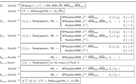
Figure 2: The sequence of games in the security proof.
G0 :Modify(0) SFsetup(1λ, n, `)→(PK,MSK,PKc,MSK[base,MSK[aux) .
Modify(2) CT?←SFEncrypt(PK, x?, Mb,PK) .c
Gk,1 :Modify(1) [βj]∅←Samp(param), SKj←
SFKeyGen(MSK, f(j),MSK[base, − ,3,[βj]∅) ifj < k SFKeyGen(MSK, f(j),MSK[
base,MSK[aux,1, − ) ifj=k
KeyGen(MSK, f(j)) ifj > k
Gk,2 :Modify(1) [βj]∅←Samp(param), SKj←
SFKeyGen(MSK, f(j),MSK[
base, − ,3,[βj]∅) ifj < k SFKeyGen(MSK, f(j),MSK[base,MSK[aux,2,[βj]∅) ifj=k
KeyGen(MSK, f(j)) ifj > k
Gk,3 :Modify(1) [βj]∅←Samp(param), SKj← (
SFKeyGen(MSK, f(j),MSK[base, − ,3,[βj]∅) ifj≤k
KeyGen(MSK, f(j)) ifj > k
Gq1+1:Modify
(3)
SKj← SFKeyGen(MSK, f(j),MSK[base,MSK[aux,1, − )
Gq1+2:Insert [β]∅ ←Samp(param) at the begin of Phase 2.
Modify(3) SK
j← SFKeyGen(MSK, f(j),MSK[base,MSK[aux,2,[β]∅ )
Gq1+3:Modify
(3) SK
j← SFKeyGen(MSK, f(j),MSK[base, − ,3,[β]∅ )
Gfinal:Modify(2) M ← {0$ ,1}λ,CT?←SFEncrypt(PK, x?, M,PK) .c
7.1 Security Theorem and Proof Overview
We obtain the following security theorem for our KP-ABE for circuits. We recall that Fn,` is the
class of polynomial size circuits with bounded input-size nand bounded depth`.
Theorem 1. Suppose that the SD1,SD2,EMDDH1,EMDDH2 Assumptions hold. Then our KP-ABE for circuits is fully secure. More precisely, for any PPT adversary A that attacks our KP-ABE for circuits in Fn,`, there exist PPT algorithms B1,B2,B3,B4, whose running times are that
of A plus some polynomial times, such that for any λ,
AdvA(n,`)-KPABE(λ)≤AdvSDB11(λ) + (2q1+ 2)AdvSDB22(λ) +q1Adv(B`,m3 )-EMDDH1(λ) +Adv`-BEMDDH4 2(λ),
whereq1 is the number of key queries byAin phase 1, andm is the maximum number of (internal)
gates per layer of circuits for which A issues key queries in phase 1.
Security Proof Structure for Theorem 1. We use a sequence of games in the following order:
Greal G0 G1,1
· · ·
Gk−1,3 Gk,1 Gk,2 Gk,3
· · ·
Gq1,3 Gq1+1 Gq1+2 Gq1+3 Gfinal
SD1
12
SD2
13
EMDDH1
3
SD2
14
SD2
15
EMDDH2
16
SD2
17
=
18
where each game is defined as follows. Greal is the actual security game, and each of the following game is defined exactly asits previous game in the sequence except the specified modification that is defined in Fig. 2. For notational purpose, let G0,3 := G0. In the final game, the advantage of
Outline for the Proof of Each Lemma. We first consider the proofs for game transitions that are based on subgroup decision assumptions (SD1,SD2): which are the game pair Greal/G0,
Gk−1,3/Gk,1,Gk,2/Gk,3,Gq1,3/Gq1+1,Gq1+2/Gq1+3. Although some of these proofs are lengthy, they all share the same idea. We thus summarize their proof sketch together below (§7.2) and postpone each of the full proofs to §B(Lemma 12,13,14,15,17 respectively).
The most non-trivial proofs are indistinguishability of Gk,1/Gk,2 and of Gq1+1/Gq1+2. Both transitions switch semi-functional keys from type-1 (the correlated type) to type 2 (an uncorrelated type). When the switching occurs in the phase 1 (corresponding to game Gk,1/Gk,2), we will
essentially use the co-selective security techniques. We will not, however, explicitly show it in a modular manner here. Instead, we reduce the indistinguishability directly to the assumption (EMDDH1). Nevertheless, the proof will exhibit clearly the nature of co-selective type of proof. That is, the adversary A first announces circuit f, the reduction algorithm B then simulates parameters (in semi-functional space) and SKf. The key is then returned to A. After then, Ain
the challenge phase will ask for ciphertext for x?, and B simulates it in the consistent way with SKf based on the simulated parameters. The proof for co-selective security of ABE for circuits is
the main novelty in this paper. Hence, we show the full proof in the paper body below in §7.3. On the other hand, if the switching occurs in the phase 2 (corresponding to gameGq1+1/Gq1+2), we will essentially, but again implicitly, use the selective security techniques, and hence we can follow from the selective security proof of the GGHSW KP-ABE [9], upon which our scheme is constructed. We prove it directly to the`-EMDDH2 assumption. We postpone this proof to§B.5.
Finally, it is easy to see that Gq1+3 is the same as Gfinal, due to the fact that all the semi-functional keys become those of uncorrelated type. We clarify the detail in Lemma18 in§B.7.
We define GjAdvA(n,`)-KPABE(λ) to be the advantage ofAin the gameGj.
7.2 Sketch of Proofs for Subgroup-Decision Based Transitions
Lemma 2 (informal). Consider pairs of games: Greal/G0, Gk−1,3/Gk,1, Gk,2/Gk,3, Gq1,3/Gq1+1,
Gq1+2/Gq1+3. If there exists an adversaryAthat has non-negligible difference in advantage between the two games in question, then we can construct an algorithm B that breaksSD1 in the first case, and SD2 in all the other four cases.
Proof Sketch. The algorithm B obtains an input (D, Z) from the underlying assumption (SD1 in the first case,SD2 in all the other cases). Bwill use the adversaryAagainst either of the two games in question as subroutines to answer whetherZ hasZN2 component being zero or random. All the proofs simulate the setup phase in exactly the same way. First, B samples [ ˜α]∅ ← Samp(param)
and sets [α]1[`,+22 ,3`]= [ ˜α]∅·[b]1[`,+22 ,3`]forMSK, and [α]1[1,3`]= [α][1`,+22 ,3`]·[ 1 ]1[1,`+1]forPK. The other
terms in PK are trivially computed: for each variable y in H := {h1, . . . , hn, φ1, φ2}, B samples [ ˜y]∅ ← Samp(param) and computes [y]1S = [ ˜y]∅ ·[ 1 ]1S for every needed term in PK,MSK. Note
that [ 1 ]1S is computable from [ 1 ]1{i},[ 1 ]3{i} for alli∈[1,3`]. On the other hand,Bcannot simulate
c
PK,MSK[base,MSK[auxsince it does not possess any [ 1 ]2S. However, weimplicitly define [ ˆy]2S= [ ˜y]∅·
[ 1 ]2Sfor each variable ˆy∈Hˆ :={ˆh1, . . . ,ˆhn,φˆ1,φˆ2}. Due to CRT,y= ˜ymodN1 and ˆy= ˜ymodN2 is independent as required. This allows B to simulate ciphertexts and keys by multiplying [ ˜y]∅
with, say F being [X]1S or [X]1S,2 (for some X). If F = [X]1S, then [ ˜y]∅·F = [yX]1S produces
Table 1: Summary of proofs for subgroup-decision based transitions (for Lemma2).
Between Difference Assumption MSK SKjin phase 1 CT SKjin phase 2
(j<k) (j=k) (j>k) (∀j)
Greal /G0 CT = normal/semi SD1 B X Z X
Gk−1,3/Gk,1 SKk = normal/semi-1 SD2 B C Z X A X
Gk,2 /Gk,3 SKk = semi-2 /semi-3 SD2 B C Z, C X A X
Gq1,3 /Gq1+1 SK∀j= normal/semi-1 SD2 B C A Z
Gq1+2/Gq1+3 SK∀j= semi-2 /semi-3 SD2 B C A Z, C
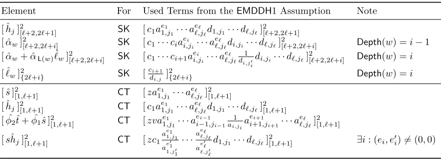
Table 2: Overview for Simulation of Elements in Lemma3
Element For Used Terms from theEMDDH1 Assumption Note
[ ˆhj]2[`+2,2`+1] SK [c1ae11,j1· · ·a e`
`,j`d1,j1· · ·d`,j`]
2
[`+2,2`+1] [ ˆαw]2[`+2,2`+i] SK [c1· · ·ciaei,jii· · ·a
e`
`,j`di,ji· · ·d`,j`]
2
[`+2,2`+i] Depth(w) =i−1 [ ˆαw+ ˆαL(w)`ˆw]2[`+2,2`+i] SK [c1· · ·ci+1aei,jii· · ·a
e`
`,j`
1 di,j0
i
di,ji· · ·d`,j`]
2
[`+2,2`+i] Depth(w) =i
[ ˆ`w]2{2`+i} SK [cdi+1
i,j ]
2
{2`+i} Depth(w) =i
[ ˆs]2
[1,`+1] CT [za
e1
1,j1· · ·a e`
`,j`]
2 [1,`+1] [ ˆhj]2[1,`+1] CT [c1ae11,j1· · ·a
e`
`,j`d1,j1· · ·d`,j`]
2 [1,`+1] [ ˆφ2ˆt+ ˆφ1sˆ]2[1,`+1] CT [zva
e1
1,j1· · ·a ei−1 i−1,ji−1
1 ai,jia
ei+1
i+1,ji+1· · ·a e`
`,j`]
2 [1,`+1]
[sˆhj]2[1,`+1] CT [zc1 ae1
1,j1 ae
0 1 1,j01
· · ·a
e` `,j`
ae
0
` `,j0`
d1,j1· · ·d`,j`]
2
[1,`+1] ∃i: (ei, e
0
i)6= (0,0)
how we use elementsZ, A, B, C from the assumptionSD1,SD2 to simulate what elements in the five game transitions that is based onSD1,SD2. Xmeans that we can trivially compute. We note that type-3 keys are exactly like normal keys but with additional [β]2`+2,3` inD1; this can be simulated using C. Also note that transitions of keys in phase 2 differ from those of phase 1 in that instead switching one key at a time, all key queries (in phase 2) are changed altogether at once.
7.3 Proof for Transition of Type-1 to Type-2 Semi-functional Key in Phase 1
Lemma 3 (Gk,1 toGk,2). For any adversaryAthat makes thek-th key query for a circuit of which
the maximum number of (internal) gates per layer ism, there exists an algorithmB that breaks the
(`, m)-EMDDH1 with |Gk,1Adv
(n,`)-KPABE
A (λ)−Gk,2Adv
(n,`)-KPABE
A (λ)| ≤AdvB(`,m)-EMDDH1(λ).
Proof Overview. The algorithmBobtains an input (D, Z) from the (`, m)-EMDDH1 Assumption. DenoteZ = [δ+c1· · ·c`+1b][2`+2,3`]. Its task is to guess whetherδ = 0 orδ ∈RR. The idea is that
B will define βk = δ in the simulation for the k-th key, so that ifδ = 0, it will be a type-1
semi-functional key, otherwise δ is random, and it will be a type-2 semi-functional key. B will construct the normal component as in the scheme while it will simulate all the semi-functional components by using the assumption. B will not define all the hatted variables (and hence, PKc,MSK[aux) until