R E S E A R C H
Open Access
Iterative robust adaptive beamforming
Yang Li
1,2*, Hong Ma
2and Li Cheng
1,2Abstract
The minimum power distortionless response beamformer has a good interference rejection capability, but the desired signal will be suppressed if signal steering vector or data covariance matrix is not precise. The worst-case performance optimization-based robust adaptive beamformer (WCB) has been developed to solve this problem. However, the solution of WCB cannot be expressed in a closed form, and its performance is affected by a prior parameter, which is the steering vector error norm bound of the desired signal. In this paper, we derive an approximate diagonal loading expression of WCB. This expression reveals a feedback loop relationship between steering vector and weight vector. Then, a novel robust adaptive beamformer is developed based on the iterative implementation of this feedback loop. Theoretical analysis indicates that as the iterative step increases, the performance of the proposed beamformer gets better and the iteration converges. Furthermore, the proposed beamformer does not subject to the steering vector error norm bound constraint. Simulation examples show that the proposed beamformer has better performance than some classical and similar beamformers.
Keywords: Array signal processing, Robust adaptive beamforming, Steering vector error, Diagonal loading
1 Introduction
The minimum variance distortionless response (MVDR) beamformer is capable of maximizing the output signal to interference-plus-noise ratio (SINR). The MVDR requires using the interference-plus-noise covariance matrix; how-ever, in many applications, it is impossible to obtain it. When the training data contains the desired signal com-ponent, the MVDR beamformer becomes the minimum power distortionless response (MPDR) beamformer [1, 2]. The MVDR beamformer maximizes the output SINR by minimizing the total beamformer output power, subject to a distortionless constraint for the desired signal. However, due to the desired signal component, even small error in the steering vector or covariance matrix can lead to severe performance degradation [3], this phenomenon is often called desired signal cancellation. In practice, many fac-tors can lead to steering vector estimation errors, such as inaccurate signal model [4], direction of arrival (DOA) estimation error [5], array perturbations [6], and calibra-tion errors [7]. Finite sample snapshots [8] lead to an inaccurate data covariance matrix. Therefore, a robust
*Correspondence: [email protected]
1School of Electrical and Information Engineering, Wuhan Institute of
Technology, 693 Xiongchu Avenue, Wuhan 430073, China
2School of Electric Information and Communications, Huazhong University of
Science and Technology, 1037 Luoyu Road, Wuhan 430074, China
technology is required to overcome these problems. We refer to adaptive beamformer that attempts to preserve good performance in the presence of steering vector or covariance matrix error as robust adaptive beamformer (RAB).
In the past two decades, many technologies have been developed to improve the robustness of the MPDR beam-former against the steering vector error. For example, the class of diagonal loading technology [9, 10] aug-ment the data covariance with a constant improves the robustness; the worst-case performance optimization-based beamformer (WCB) [11, 12] restrains the gain in signal uncertainty range that is larger than one; the covariance fitting-based beamformer [13, 14] solves a new steering vector which is fitting for the sample covariance matrix to avoid desired signal cancellation; the magnitude response constraints method [15, 16] improves the robust-ness by restraining the main beam pattern; the covariance matrix reconstruction approach [17, 18] eliminates the signal component from the data covariance matrix to prevent desired signal cancellation.
The classical WCB [11] minimizing the total beam-former output power, subject to the gain in desired signal steering vector’s uncertainty set, is larger than one. The
WCB has a good robustness performance, but it has two inherent drawbacks. On the one hand, the constrained optimization equation of WCB is a nonconvex NP-hard problem; although there exists many methods [12, 19] to solve it, there is no closed-form solution until now. On the other hand, the performance of WCB is highly affected by the prior value of steering vector error norm bound. Unfortunately, the optimum bound value [20, 21] cannot be obtained in practice, and if the prior value is not big enough, the performance of WCB will decrease significantly.
To solve these two problems of WCB, we propose a novel beamformer; its idea and way are as follows. Firstly, we propose an approximate diagonal loading expression of WCB under certain conditions. Then, we build a feed-back loop relationship between steering vector and weight vector based on this expression. At last, a novel RAB is developed based on the iterative implementation of this feedback loop.
The outline of this paper is as follows. The data model and background on adaptive beamforming are provided in Section 2. The proposed beamformer and its implemen-tation are developed in Section 3. The simulation results are presented in Section 4. Finally, a brief conclusion appears in Section 5. In the paper,E[],()H,()−1,, and ⊥ denote the expectation, Hermitian transpose, inverse, the two-norm, and orthogonal, respectively; superscriptˆ denotes the estimated value.
2 Problem formulation
2.1 The MPDR beamformer
Considering a uniform linear array (ULA) withM
omni-directional sensors, one desired signal andLinterference signals impinging upon the array from different direc-tions, and the source is in the far-field of the array. The received array signal can be expressed as
x(k)=aSsS(k)+ L
i=1
aisi(k)+n(k) (1)
where x(k), a, and n(k) are M× 1 complex vector, k denotes the snapshot number, andai,i=S, 1,. . .,Lis the actual steering vector of thei-th signal.si(k)is zero-mean stationary i-th signal;n(k) denotes the noise. Assuming that each signal and noise are statistically independent, the data covariance matrix of the array output is given by
R=E[x(k)xH(k)]=PSaSaHS + L
i=1
PiaiaHi +PNI (2)
wherePS,Pi, andPN denote the power of desired signal, i-th interference, and noise, respectively.
The beamformer output signal can be written as
y(k)=wHx(k) (3)
where wis the weighing vector of the beamformer. The
MPDR beamformer is mathematically equivalent to the problem
min
w w
HRws.t.wHa
S=1 (4)
The solution of MPDR is often called optimum weight
wMPDR= R
−1a S
aHSR−1a S
(5)
However, we cannot achieve the optimum weight in practice due to two inaccurate parameters. On the one hand, since data covariance matrixRis unknown in
prac-tice, it is replaced by K snapshots sample covariance
matrixRˆ = K1
K
k=1
x(k)xH(k). On the other hand, steering vectoraSrelates to signal frequency, direction of arrival, sensors locations, coupling effect, as well as other factors, any inaccurate of these factors can lead to steering vector error.
If the signal-to-noise ratio (SNR) of desired signal is high, even slight error of Ror aS will cause the MPDR beamformer suppresses the desired signal as an inter-ference, which leads to a severe degradation of the per-formance [3]. This effect is often called desired signal cancellation.
This paper only concerns about the error of steering vector, so we use actual covariance matrixRin all of the following formulas.
2.2 The worst-case performance optimization-based beamformer
The WCB [11] minimizing the total beamformer output power, subject to the gain in desired signal steering vec-tor’s uncertainty set, is larger than one. In rank-one signal and spherical uncertainty set case [22], the WCB can be expressed as
min
w w
HRw
s.t.wH(aˆS+a)≥1, for all a ≤ε
(6)
whereaˆSis the assumed steering vector of desired signal (obtained from estimated DOA and nominal array man-ifold). The prior known positive constant ε [20] can be explained as a norm bound of the unknown error between
aSandaˆS.
min
w w
HRw
s.t.wHaˆS−εw =1
(7)
There are many methods to solve the problem above, such as, the convex optimization tools solve method [11], the eigen-decomposition root-searching method [19], the diagonal loading method [23], the recursive implementa-tion [12], etc.
2.3 Approximate diagonal loading solution of the WCB
Using the Lagrange multiplier method, problem (7) can be written as
F(w,λ)=wHRw−λ(wHaˆS−εw −1) (8) whereλis the Lagrange multiplier. Differentiating (8) with
wand equating the result to zero, we obtain the following equation:
Rw+λε w
w =λˆaS (9)
Using the fact that multiplying the weight vector by any arbitrary constant does not change the output SINR, we can transform (9) to
Rw+ε w
w = ˆaS (10)
So that (10) does not contain the Lagrange multiplier anymore. Then, (10) can be written as
w=
R+ ε
wI
−1 ˆ
aS (11) It can be seen from (11) that the WCB belongs to the class of diagonal loading. Taking the norm squared of the both sides of (11), and defining the diagonal loading level ρ=ε/w, we obtain
ε
ρ
2
=(R+ρI)−1aˆS2 (12)
In the following, we will solve (12). The solve idea takes reference to [9, 23], and [24]. Using Woodbury formula of matrix inverse, we have
(R+ρI)−1
= PSaSaHS +(RIN+ρI)
−1
=(RIN+ρI)−1−
PS(RIN+ρI)−1aSaHS(RIN+ρI)−1 1+PSaHS(RIN+ρI)−1aS
(13)
whereRIN=Li=1PiaiaHi +PNIis interference-plus-noise covariance matrix.RIN can be expressed in eigen decom-position form as
RIN=UIIUIH+UNNUHN= L
i=1
γiuiuHi +PN M
i=L+1
uiuHi (14)
where γi and ui are the eigenvalues and corresponding eigenvectors of RIN, eigenvalues are sorted in
descend-ing order, γ1 ≥ . . . ≥ γL γL+1 = . . . =
γM = PN,UI =[u1,. . .,uL] spans the interference sub-space,UN =[uL+1,. . .,uM] spans the noise subspace, and
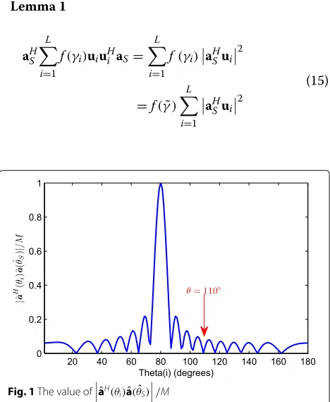
UIUHI +UNUHN=I,span{ai} =span{ui},i=1, 2,. . .L[7]. When DOA separation between signal and interference is larger than a beam width,aHSai/M 1,i = 1,. . .,L [25] (Fig. 1 gives an example). Assuming this condition always holds, we can make the approximationaHSui2 MandaHSUIUHI aS M, which can be further expanded toaHSUNUHNaS =aHS(I−UIUHI )aS =M−aHSUIUHI aS≈ M, andUHIaS2UHNaS2.
It is well known that the desired signal’s steering vector aS is orthogonal to the noise subspace of data covariance matrix R. The result aHSUNUHNaS ≈ M
reveals a new property: aS approximately belongs to
the noise subspace of interference-plus-noise covariance
matrix RIN. The precondition is that the DOA
sepa-ration between desired signal and interference is larger than a beam width; this condition holds under normal conditions.
The following Lemma 1 is used in this paper:
Lemma 1
aHS
L
i=1
f(γi)uiuHi aS= L
i=1
f(γi)aHSui2
=f(γ )˜ L
i=1
aHSui2
(15)
where f(·)is a monotonic function in this paper, andγ1> ˜
γ > γLPN always holds. Lemma1is obvious, and it is easy to be proved, so we use this lemma directly.
Using Lemma 1, and definingf(γ )=1/(γ+ρ), we have can be simplified as
aHS(RIN+ρI)−1aS≈ M, which can be further extended to
aHS(RIN+ρI)−1aˆS≈ ˆaHS(RIN+ρI)−1aˆS≈ M PN+ρ =κ
(18)
Similar to (16) and (17), we can obtain the following approximations
According to (13), (18), (19), and (20), the following approximation holds
The approximate diagonal loading level can be solved by using (12) and (21) as
ρ≈ ε (MP√ S+PN)
M−ε (22)
Finally, the weight vector of WCB is
wWCB=(R+ρI)−1aˆS (23)
Equation (22) indicates that the diagonal loading level relates to the desired signal’s powerPS, noise powerPN,
and steering vector error norm bound ε. The premise
behind (22) is the Eqs. (18), (19), and (20). If aˆS = aS, (18), (19), and (20) are strictly true and (22) is reliable. If there exists error betweenaˆSandaS, the following iter-ative method will reduce this error step by step so as to make (22) reliable.
3 The proposed beamformer
The key problem of (22) is how to obtain the accurate value ofMPS+PN, or reliable approximate value, and how to set a suitableε. The idea of the proposed beamformer is to use iterative implementation. Firstly, we estimate an approximate value ofMPS+PN, and a prior value ofε, to obtain the weight vector. Then, we estimate a more accurate value of MPS + PN by using this weight vec-tor. Repeating this process, it is maybe possible that the updatedMPS+PNapproaches to its actual value.
3.1 Feedback loop relationship between steering vector and weight vector
Under the condition that the interferences are absent, the data covariance matrix becomesR = PSaSaHS +PNI. Its inverse is calculated by
R−1= 1
Equation (25) reveals the relationship between steering vectoraSandMPS+PN.
In practice,aSis replaced byaˆSfor MPDR beamformer in (5). For a weight vector obtained by WCB or other beamformers, we can define an “equivalent steering vec-tor” for MPDR beamformer. For example, by combining (5) and (23), we can establish the following relationship
α(R+ρI)−1aˆS=αwWCB=wWCB−MPDR=
where α is a constant, a˜S is an equivalent steering vec-tor for MPDR beamformer, and we guess thata˜Sis more accurate thanaˆSifwWCB(obtained by (23)) is better than
wMPDR(obtained by (5) withaˆS).
It is easy to expressa˜SbyRandwfrom (26) [26] ˜
aS=αRwWCB (27) whereα =αa˜HSR−1a˜S. The equivalent steering vectora˜S should be scaled by the fact that the norm ofa˜S equals √
Henceforth, we obtain the feedback loop relationship between steering vectoraS, diagonal loading levelρ, and weight vectorwthrough (22), (23), (25), and (28).
3.2 Iterative implementation
If thea˜Sobtained by (28) is closer to actual value thanaˆS, we preliminary think that the following iteration imple-mentation will obtain a better steering vector and simul-taneously obtain a better weight vector, step by step.
Initialization:a(0)= ˆaS for k=1, 2,. . .
τ =Mε/√M−ε, p(k)=1/a(k−1)HR−1a(k−1)
w(k)=R+τp(k)I−1a(k−1) a(k)=Rw(k),a(k)=√Ma(k)/a(k)
We call this iterative implementation as iterative robust adaptive beamformer (IRAB).
3.3 The performance proof of IRAB
The following two properties hold for the proposed IRAB:
Property 1a(k)−aS
ProofThe data covariance matrix Rcan be written in eigen-decomposition form as
where ri and qi are the eigenvalues and corresponding eigenvectors of R, eigenvalues are sorted in descending
order r1 ≥ . . . ≥ rL+1 rL+2 = . . . = rM =
The weight vector ofk-th iterative step can be expressed byaanda⊥as
where μ1 is a constraint constant which subject to
We can obtain the following result from (29) and (30)
From (31), (34), and (35), we can obtain
a(k)=μ1 steering vector per iterative step is
steering vector is obtained.
Property 2 SINR(k)>SINR(k−1)for each iterative step, and SINR has an upper bound.
Proof
Similar to Lemma 1, we have
w(k)HRw(k)
3.4 Some remarks on the IRAB
3.4.1 The setting of prior parameter
Equation (22) indicates that not onlyMPS+PN but also the prior parameterεcan affect the diagonal loading level.
Many existed RABs use the constraint conditiona ≤
ε, so they face the same problem: how to set a suitableε? Jian Li suggest thatεshould be chosen as small as pos-sible butε ≥ ε0=min
φ aˆSe
jφ−a
S[20]. If ε < ε0, the
desired signal will be suppressed as interference. Ifε is chosen much larger thanε0, the ability of beamformer to suppress interferences that are close to the desired signal will degrade.
The parameter τ is defined in the implementation of
IRAB in Section 3.2. It can be seen from (37) that, ifτ >0, the two properties of IRAB will always hold, which indi-cates that the iteration will always converge ifε < √M. Therefore, theεdoes no longer subject to the constraint ε≥ε0; any 0< ε <
√
Mis suitable for IRAB. Notice that the value of ε0(k)=min
φ a
(k)ejφ−a S will
decrease and approach to zero as the iterative step increases and theεis better to be decreased as the itera-tion time increases. An experiential way is to reduceεby half per iterative step. Thus, the proposed IRAB can be modified as follows
3.4.2 The stopping criterion
The iteration should be stopped under certain criterions, and the performance should not deteriorate on special occasions. On the one hand, three parameters are updated as the iterative step increases, thep(k),w(k), anda(k). The p(k) relates toa(k−1), thew(k) relates top(k), anda(k−1), thea(k)relates tow(k). Therefore, we can make the stop-ping criterion only by the parametera. Ifa(k)changes less than a threshold, such as a very smallδ, with respect to
a(k−1), we consider the iteration converges. Wei Jin uses
a(k)−a(k−1) ≤ δ as the stopping criterion [26]. How-ever, because the phase rotate ofadoes not affect the per-formance of beamformer, using min
φ a
(k)−a(k−1)ejφ≤ δis better, but the amount of calculation is increased.
As the norm ofa(k)anda(k−1)are both equal to√M, the stopping criterion 1 of IRAB is as follows
a(k)Ha(k−1)/M≥0.999999 (43)
It is obvious that the smaller difference between a(k)
anda(k−1) is, the larger of the value of a(k)Ha(k−1)is; the maximum value ofa(k)Ha(k−1)equals toMifa(k) = a(k−1)ejφ; the phase rotate ofadoes not affect the value of
a(k)Ha(k−1).
On the other hand, two scenes should be considered. Firstly, when SNR of desired signal is very low, the updated steering vector cannot be able to converge to its actual value, even if it may converge to interferences or noise peaks. To avoid the desired signal’s steering vector devi-ating its actual value too large, we add the following stopping criterion 2 [27]
whereθSˆ is the prior DOA of desired signal andθW is the uncertainty range. Stopping criterion 2 is based on the fact that, if|θi−θS| is larger,aˆH(θi)ˆa(θS)ˆ is smaller (Fig. 1 shows an example, ignore the ripple). Therefore, the iter-ation stops when the corresponding DOA ofa(k)is out of uncertainty range.
However, these two stopping criterions have a defect. When angular separation betweenθiandθSˆ is larger than a beam width, aˆH(θi)aˆ(θS)ˆ M, i = 1,. . .,L. At some specific angles, aˆH(θi)aˆ(θS)ˆ approaches to zero.
Using a ULA withM=16 as example, we plot the value
happens to be equal to 110◦, [a(k)+ ˆa(110◦)]Haˆ(θS)ˆ ≈
a(k)Haˆ(θS)ˆ , thus the stopping criterion 2 may not work, and it does not affect the stopping criterion 1, which fur-ther means the updated steering vector may converge to the sum of desired signal and interferences. To deal with this special case, we add the following stopping criterion 3
a(k)− ˆaθSˆ >maxa(k)− ˆa
ˆ θS+θW
2
,a(k)− ˆa
ˆ θS− θW
2
(45)
Stopping criterion 3 is based on the fact that ifθi− ˆθS
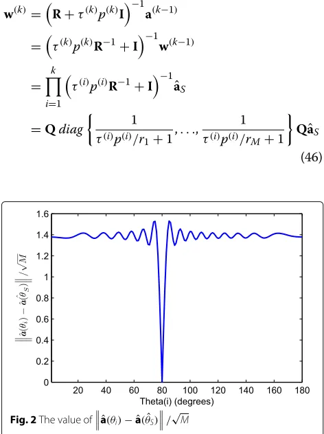
is larger than a threshold,aˆ(θi)− ˆa(θS)ˆ is large. Figure 2 shows the value ofaˆ(θi)− ˆa(θS)ˆ /√M,θSˆ = 82◦,θi = 1 : 180◦ for a ULA with M=16. Once the interferences component ina(k)surplus threshold, the iteration stops. 3.4.3 The IRAB does not belong to the class of diagonal
loading
When the iteration stops atk-th step, the weight vector of IRAB is
w(k)=
R+τ(k)p(k)I
−1
a(k−1)
=τ(k)p(k)R−1+I−1w(k−1)
= k
i=1
τ(i)p(i)R−1+I−1aˆ S
=Qdiag
1
τ(i)p(i)/r1+1,. . .,
1 τ(i)p(i)/rM+1
QaˆS (46)
Fig. 2The value ofaˆ(θi)− ˆa(θˆS)/
√ M
where the columns of Qcontain the eigenvectors of R. Therefore, the IRAB does not belong to the class of diag-onal loading.
3.4.4 The computational complexity
The computational complexity of IRAB is determined by the inversion of aM×Mmatrix, which is equal toO(M3), per iterative step.
3.4.5 Relationship between the IRAB and some similar beamformers
Notice that the proposed IRAB relates to the follow-ing three beamformers: the DLWCB in [23], the IWCB in [26], and the IRCB2 in [24]. Their similarities and differences are as follows: (1) the equivalent diagonal load-ing levels of IRAB, DLWCB, and IRCB2 are the same, which is derived from the method in [9]; (2) DLWCB cannot be implemented in practice while IRAB is easy to be implemented; (3) although the equivalent steer-ing vectors of IRAB and IWCB have the same form, which are deriving from Appendix B in [13], their solv-ing methods per iterative step are quite different; (4) although the equivalent diagonal loading levels of IRAB and IRCB2 are the same, and their proof methods are sim-ilar, they are based on two different methods ([11] and [13]); and (5) the stopping criterion of IRAB is different to others.
4 Simulation results
In the following simulation examples, a ULA withM=16 antennas and half-wavelength antenna spacing is consid-ered. Assume each antenna is omni-directional, the array has been calibrated and omit the coupling effect. The desired signal and interferences are stationary Gaussian random process, and the additive noise is a spatially white Gaussian process. There are two interferences with DOAs and interference-to-noise ratios (INR) of [55◦, 20 dB] and [115◦, 30 dB], respectively. One desired signal is impinging on the array from 80◦, but its prior DOA is
82◦, except example 5. The DOA uncertainty range of
desired signal is θW = 8◦. The actual norm bound
of the error between aS and aˆS is calculated by ε0 = min
φ aS− ˆaSe
jφ. 1000 runs are performed except for
example 2. The number of snapshots is 200 except for example 6.
The proposed IRAB is contrasted with some classical and similar RABs; they are as follows:
OPT: The MPDR beamformer of (5) with actualRand
aS.
Fig. 3SINR versus SNR with differenceεfor WCB
DLWCB: The diagonal loading approach of WCB, which is proposed in [23]. Its diagonal loading level has the same form with (22). Notice that the DLWCB cannot be imple-mented in practice, actualPSandPNare used to calculate the diagonal loading level in the simulations. The norm bound of steering vector error is set asεDLWCB=1.1×ε0, except for example 5.
IWCB: The iterative implementation of worst-case performance optimization-based beamformer [26]. The norm bound of steering vector error is set asεIWCB=0.1.
4.1 SINR versus steering vector error bound
The first example simulates the SINR performance affected by norm bound of steering vector error. We set
a group of different ε for WCB and IRAB. The actual
norm bound of steering vector error corresponding to
2◦ pointing error is about ε0 = 1.96. The input SNR
of desired signal changes from−20 to 40 dB. Figures 3 and 4 show the results of WCB and IRAB, respectively. Results indicate that, when εis set smaller thanε0, the SINR performance of WCB decreases rapidly, while the performance of IRAB always keep stable. The theoretical analysis in Section 3.4 that theεdoes no longer subject to the constraintε≥ε0is verified. Figure 4 also shows that,
Fig. 4SINR versus SNR with differenceεfor IRAB
Fig. 5The convergence properties of IRAB and IWCB: steering vector
error versus iterative steps
theεIRABshould be set appropriately, not too small or too large. An experience value is setεIRAB = √M/2; we use this setting in all the following examples.
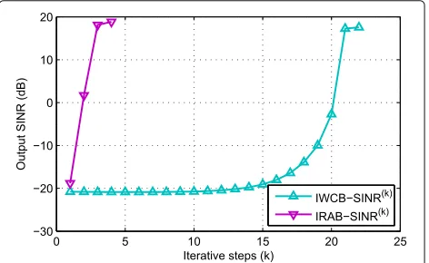
4.2 Iterative convergence property
The second example evaluates the convergence properties of IRAB and IWCB, SNR=25 dB. Figure 5 shows the norm bound error between the updated steering vector and actual steering vector per iterative steps. Figure 6 shows the updated SINR per iterative steps. Results show that as the iterative step increases, the error of updated steering vector grows smaller, and the updated SINR increases to a stable value. Additionally, the proposed IRAB has a faster convergence speed than IWCB.
4.3 Output SINR performance
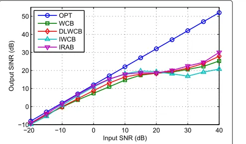
The third example evaluates the output SINR perfor-mance versus input SNR. The result in Fig. 7 shows that the proposed IRAB outperforms other RABs almost at any input SNR.
Fig. 6The convergence properties of IRAB and IWCB: SINR versus
Fig. 7Output SINR versus input SNR
4.4 Array beam pattern gain
The fourth example presents the array beam pattern gain of four RABs, SNR=25 dB. The results of Fig. 8 show that the main beam peak of IRAB and IWCB nearly points to the actual DOA of desired signal, while the WCB and DLWCB do not. The theoretical result of (37) indicates that, as the iterative step increases, theη(k)approaches to zero, thea(k)gets closer to actual value, and therefore the main beam peak points to the actual DOA. For this reason, the IRAB and IWCB have better SINR performance than
WCB and DLWCB, especially at SNR<20 dB, as shown
in Fig. 7.
4.5 SINR versus pointing error
The fifth example evaluates the SINR versus pointing
error, SNR=25 dB. SettingεWCB = εDLWCB = 2, which
corresponds to about 2◦ pointing error. The results in Fig. 9 show that the SINR performance of WCB decreases greatly when pointing error exceeds 2◦; the IRAB and IWCB exhibit stable performance in the DOA uncer-tainty rangeθW = 8◦; the DLWCB has a wilder pointing
Fig. 8Array beam pattern gain
Fig. 9Output SINR versus pointing error
error range and does not subject to the 2◦pointing error constraint.
4.6 SINR versus snapshots
We use actual data covariance matrix Rin the theoreti-cal analysis; the affect of finite sample effect with different snapshots is simulated in the sixth example, SNR=25 dB. The results in Fig. 10 show that as the snapshots increase from 16 to 400, the output SINR of WCB, DLWCB, IWCB, and IRAB increases about 7.5, 5.5, 8.0, and 7.0 dB respectively. The SINR performance of IRAB outperforms other RABs and goes to stable when snapshots number surplus 200.
4.7 SINR versus DOA separation and array size
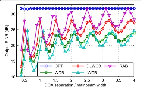
As declared in Section 2.3, the effectiveness of the proposed algorithm requires “DOA separation between desired signal and interference is larger than a beam width”. In this section, we simulate the SINR performance versus different DOA separations between desired signal and interference and versus different array size. In the sim-ulations, three arrays with element number M=10, 15, 20 are used; their mainbeam width are about 24◦, 16◦, and
Fig. 11SINR versus DOA separation: M=10, mainbeam width=24◦
12◦, respectively (calculated by conventional beamformer with weight vector equals to the steering vector of desired signal). The SNR of desired signal is 20 dB. There is only one interference with INR=15 dB. The DOA separation between desired signal and interference varies from 0.4 to 5 times of main beam width. Other parameters are the same with the parameters declared in the beginning of Section 4.
The results in Figs. 11, 12, and 13 show that there are some ripples; they are caused by the nulls of beam pattern; the performance of IRAB is better than others in most cases; the proposed IRAB can work even when DOA sep-aration between desired signal and interference is smaller than a mainbeam width (The IRAB can work with DOA separation larger than half a mainbeam width); and as the DOA separation increases, the performance of IRAB gets better.
5 Conclusions
We have derived an approximate diagonal loading solu-tion of the WCB in this paper. A novel beamformer named
Fig. 12SINR versus DOA separation: M=15, mainbeam width=16◦
Fig. 13SINR versus DOA separation: M=20, mainbeam width=12◦
IRAB have been proposed based on this solution. Theo-retical analysis indicates that the proposed IRAB has three properties: the iteration will converge; the performance gets better as the iterative step increases; the IRAB does not subject to the steering vector error norm bound con-straint and exhibits stable performance through a wide steering vector error bound range. Simulation results not only verify these properties but also show that the pro-posed IRAB outperforms other contrasted RABs under the set parameters.
Acknowledgements
The authors wish to thank the Handling Editor and Reviewers for their detailed review, which helped improve this manuscript. This work is supported by the scientific research foundation of Wuhan Institute of Technology (No. K201768).
Authors’ contributions
YL provided the idea and wrote the manuscript. HM guided this paper. LC gave some improvement suggestions. All authors read and approved the final manuscript.
Authors’ information
Yang Li received the B.S. and M.S. degrees from Wuhan University of Technology, Wuhan, China, in 2006 and 2010, respectively, and received the Ph.D. degree in Electromagnetic Field and Microwave Technology from Huazhong University of Science and Technology, Wuhan, China, in 2016. Now, he is a lecturer of School of Electrical and Information Engineering, Wuhan Institute of Technology, Wuhan, China. His current research interests include array signal processing, adaptive filtering, and radio wave propagation. Hong Ma received the B.Eng., M. Eng., and Ph.D. degrees in Electromagnetic Field and Microwave Technology from Huazhong University of Science and Technology in 1988, 1992, and 1998, respectively. He is currently a Professor of School of Electronic Information and Communications, Huazhong University of Science and Technology. His research interests include radar system, electromagnetic and microwave technology, and nonlinear system theory. Li Cheng received the B.Eng. degree in Electronic Information Engineering from Hubei University in 2002 and the M. Eng. degree in Communication and Information System from Wuhan University of Technology in 2005. Now, she is presently working on her Ph.D. degree in Electromagnetic Field and Microwave Technology in Huazhong University of Science and Technology. She is currently an associate professor of School of Electrical and Information Engineering, Wuhan Institute of Technology. Her research interests include wireless communication, radio wave propagation model, and radar signal processing.
Competing interests
Publisher’s Note
Springer Nature remains neutral with regard to jurisdictional claims in published maps and institutional affiliations.
Received: 11 January 2017 Accepted: 4 August 2017
References
1. L Harry, V Trees, Optimum array processing: part IV of detection, estimation, and modulation theory (2002). http://onlinelibrary.wiley.com/ book/10.1002/0471221104. doi:10.1002/0471221104
2. L Ehrenberg, S Gannot, A Leshem, E Zehavi, inElectrical and Electronics Engineers in Israel (IEEEI), 2010 IEEE 26th Convention Of. Sensitivity analysis of MVDR and MPDR beamformers (IEEE, 2010), pp. 000416–000420. http:// ieeexplore.ieee.org/document/5662190/. doi:10.1109/EEEI.2010.5662190 3. M Wax, Y Anu, Performance analysis of the minimum variance
beamformer in the presence of steering vector errors. Signal Processing, IEEE Transactions on.44(4), 938–947 (1996). doi:10.1109/78.492546 4. A Pezeshki, BD Van Veen, LL Scharf, H Cox, ML Nordenvaad, Eigenvalue
beamforming using a multirank mvdr beamformer and subspace selection. Sig. Process. IEEE Trans.56(5), 1954–1967 (2008). doi:10.1109/TSP.2007.912248
5. W Zhang, J Wang, S Wu, Robust capon beamforming against large doa mismatch. Signal Process.93(4), 804–810 (2013). doi:10.1016/j.sig-pro.2012.10.002
6. JH Lee, CC Wang, Adaptive array beamforming with robust capabilities under random sensor position errors. Radar, Sonar and Navigation, IEE Proc.152(6), 383–390 (2005). doi:10.1049/ip-rsn:20045018
7. C-Y Tseng, DD Feldman, LJ Griffiths, Steering vector estimation in uncalibrated arrays. Signal Proc. IEEE Trans.43(6), 1397–1412 (1995). doi:10.1109/78.388853
8. X Mestre, MA Lagunas, Finite sample size effect on minimum variance beamformers: Optimum diagonal loading factor for large arrays. Signal Proc. IEEE Trans.54(1), 69–82 (2006). doi:10.1109/TSP.2005.861052 9. F Vincent, O Besson, inRadar, Sonar and Navigation, IEE Proceedings.
Steering vector errors and diagonal loading, vol. 151 (IET, IET, 2004), pp. 337–343. doi:10.1049/ip-rsn:20041069
10. Y Selén, R Abrahamsson, P Stoica, Automatic robust adaptive beamforming via ridge regression. Signal Process.88(1), 33–49 (2008). doi:10.1016/j.sigpro.2007.07.003
11. SA Vorobyov, AB Gershman, Z-Q Luo, Robust adaptive beamforming using worst-case performance optimization: a solution to the signal mismatch problem. Signal Process. IEEE Trans.51(2), 313–324 (2003). doi:10.1109/TSP.2002.806865
12. A Elnashar, Efficient implementation of robust adaptive beamforming based on worst-case performance optimisation. IET Signal Process.2(4), 381–393 (2008). doi:10.1049/iet-spr:20070162
13. J Li, P Stoica, Z Wang, On robust Capon beamforming and diagonal loading. Signal Process. IEEE Trans.51(7), 1702–1715 (2003). doi:10.1109/TSP.2003.812831
14. A Hassanien, SA Vorobyov, KM Wong, Robust adaptive beamforming using sequential quadratic programming: an iterative solution to the mismatch problem. Signal Process. Letters IEEE.15, 733–736 (2008). doi:10.1109/LSP.2008.2001115
15. ZL Yu, MH Er, W Ser, A novel adaptive beamformer based on semidefinite programming (sdp) with magnitude response constraints. Antennas Propag. IEEE Trans.56(5), 1297–1307 (2008). doi:10.1109/TAP.2008.922644 16. D Xu, R He, F Shen, Robust beamforming with magnitude response
constraints and conjugate symmetric constraint. IEEE Commun. letters.
17(3), 561–564 (2013). doi:10.1109/LCOMM.2013.011513.122688 17. Y Gu, A Leshem, Robust adaptive beamforming based on interference
covariance matrix reconstruction and steering vector estimation. Signal Process. IEEE Trans.60(7), 3881–3885 (2012).
doi:10.1109/TSP.2012.2194289
18. Z Zhang, W Liu, W Leng, A Wang, H Shi, Interference-plus-noise covariance matrix reconstruction via spatial power spectrum sampling for robust adaptive beamforming. IEEE Signal Process. Letters.23(1), 121–125 (2016). doi:10.1109/LSP.2015.2504954
19. K Zarifi, S Shahbazpanahi, AB Gershman, Z-Q Luo, Robust blind multiuser detection based on the worst-case performance optimization of the
mmse receiver. Signal Process. IEEE Trans.53(1), 295–305 (2005). doi:10.1109/TSP.2004.838932
20. P Stoica, Z Wang, J Li, Robust capon beamforming. Signal Process. Letters IEEE.10(6), 172–175 (2003). doi:10.1109/LSP.2003.811637
21. JP Lie, W Ser, CMS See, Adaptive uncertainty based iterative robust capon beamformer using steering vector mismatch estimation. Signal Process. IEEE Trans.59(9), 4483–4488 (2011). doi:10.1109/TSP.2011.2157500 22. RG Lorenz, SP Boyd, Robust minimum variance beamforming. Signal
Process. IEEE Trans.53(5), 1684–1696 (2005). doi:10.1109/TSP.2005.845436 23. J-r Lin, Q-c Peng, H-z Shao, On diagonal loading for robust adaptive
beamforming based on worst-case performance optimization. ETRI journal.29(1), 50–58 (2007). doi:10.4218/etrij.07.0105.0186
24. Y Li, H Ma, D Yu, L Cheng, Iterative robust capon beamforming. Signal Process.118, 211–220 (2016). doi:10.1016/j.sigpro.2015.07.004 25. L Chang, C-C Yeh, Performance of dmi and eigenspace-based
beamformers. Antennas Propag. IEEE Trans.40(11), 1336–1347 (1992). doi:10.1109/8.202711
26. W Jin, W Jia, M Yao, S Zhou, Robust adaptive beamforming based on iterative implementation of worst-case performance optimisation. Electron. letters.48(22), 1389–1391 (2012). doi:10.1049/el.2012.1718 27. SE Nai, W Ser, ZL Yu, H Chen, Iterative robust minimum variance