Digital image compression on parallel computer architectures

ON PARALLEL COMPUTER

ARCHITECTURES

SAVITRIDEVI BEVINAKOPPA

A thesis submitted in fulfillment of the requirements for the

Degree of Doctor of Philosophy in Science

VICTORIA °

UNIVERSITY

_/^^"''o^^

^ f - LiaRAr.Y ;•

\ ^ _{r • y}

° \'^'^ .^"./

-^

Department of Computer and Mathematical Sciences

Faculty of Science

Victoria University of Technology

Melbourne

30001005117116 .

Bevinakoppa. Savitndevi G

Digital image compression on

parallel computer

Certified that the dissertation entitled "Digital Image Compression on

Parallel Computer Architectures", which is being submitted by Savitridevi

Bevinakoppa in fulfilment for the award of the Degree of Doctor of

Philosophy in Science of the Victoria University of Technology, is a

record of the student's own work carried out by her under our joint

supervision and guidance. The matter embodied in this dissertation has not

been submitted for the award of any other Degree or Diploma.

Q^^Lh^

Victoria University of Technology

Main aim of this project is to investigate the application of parallel processing

techniques to digital image compression. Digital image compression is used to reduce

the number of bits required to store an image in computer memory and/or transmit it

over a communication link. Over the past decade advancements in technology have

spawned many applications of digital imaging, such as photo videotex, desktop

publishing, graphics arts, colour facsimile, newspaper wirephoto transmission, medical

imaging. For many other contemporary applications, such as distributed multimedia

systems rapid transmission of images is necessary. Dollar cost as well as time cost of

transmission and storage tend to be directly proportional to the volume of data.

Therefore, application of digital image compression techniques become necessary to

minimise costs.

A number of digital image compression algorithms have been developed and

standardised. With the success of these algorithms, research effort is now directed

towards improving implementation techniques. Joint Photographic Experts Group

(JPEG) and Motion Photographic Experts Group (MPEG) are international

organisations which have developed digital image compression standards. Hardware

(VLSI chips) which implement the JPEG image compression algorithm are available.

Such hardware is specific to image compression only and can not be used for other

image processing applications. A flexible means of implementing digital image

compression algorithms is still required. An obvious method of processing different

imaging applications on general purpose hardware platforms is to develop software

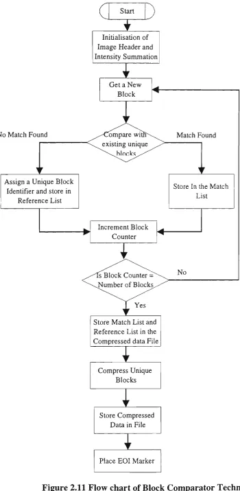
These blocks are processed sequentially. There is always a possibility of having similar

blocks in a given image. If similar blocks in an image is located, then repeated

compression of these blocks is not necessary. By locating similar blocks in the image,

speed of compression can be increased and the size of compressed image can be

reduced. Based on this concept an enhancement to the JPEG algorithm is proposed,

called Block Comparator Technique (BCT).

Most of the current implementation of JPEG and MPEG compression methods are in

sequential form. Parallel processors are becoming more affordable and are likely to be

used quite extensively in the near future. Therefore various options for implementing

digital image compression algorithms were investigated on parallel computer

ACKNOWLEDGMENTS

First and foremost I would like to express my appreciation and my sincere gratitude to my supervisors Dr. Nalin K. Sharda and Dr. Hema Sharda, without whose constant support and help this thesis could not have been completed. Their inspiration, enthusiasm and encouragement have made this research successfiil.

I wish to thank my husband Gangadhar and my daughters Megha and Manisha for their love and support over the years. My special thanks to my father V. B. Nandi who encouraged me to undertake this research which was both challenging and rewarding.

I would like to thank the Department of Computer System Engineering, RMIT, Melbourne for providing the Mercury system, Defence Science and Technology Organisation (DSTO), Adelaide for their contribution to the Shiva system installed in the Department of Computer and Mathematical Sciences, Victoria University of Technology. I would also like to thank Dr. Vijay Bhatkar, Sampath, Suhas and other staff members at Centre of Development of Advanced Technology (C-DAC), Pune, India for their support and assistance carrying out the comparitive studies on the Param supercomputer.

CONTENTS - BRIEF

Abstract i Acknowledgement iii

List of Figures xi List of Tables xvi List of Notations xxi

1 INTRODUCTION

1.1 Introduction 2 1.2 Problem Statement 2

1.3 Literature Review 3 1.4 Research Objectives 7 1.5 Thesis Outline 8

2 DIGITAL IMAGE COMPRESSION TECHNIQUES

2.1 Introduction 11 2.2 Digital Image Compression Techniques 11

2.3 JPEG Standard 15 2.4 Block Comparator Enhancement to the JPEG Algorithm 29

2.5 Summary 63

3 PARALLEL PROCESSING PLANS FOR DIGITAL IMAGE

COMPRESSION TECHNIQUES

3.1 Introduction 65 3.2 Parallel Computer Architectures 65

3.3 Parallel Processing Plans for Digital Image Compression Techniques 72

3.4 Implementation of Plans on Parallel Computer Architectures 76

3.5 Performance Measures 83

3.6 Summary 84

4 IMPLEMENTATION OF JPEG ALGORITHM ON PARALLEL

COMPUTERS

4.1 Introduction 86 4.2 Implementation of the JPEG Algorithm on the Mercury System 86

4.3 Implementation of the JPEG Algorithm on the Shiva System 94 4.4 Implementation of the JPEG Algorithm on the Param System 104

4.5 Performance Comparison of Parallel Computers I l l

5.1 Introduction 124 5.2 Simulation Procedure 124

5.3 Simulation Results of Digital Image Compression Techniques 144

5.4 Performance Comparison of Parallel Architectures 155

5.5 Summary 165

6 CONCLUSIONS

6.1 Introduction 167 6.2 Block Comparator Technique Enhancement to the JPEG Algorithm 167

6.3 Implementation of the Digital Image Compression Algorithm 171

6.4 Simulation of Digital Image Compression 172

6.5 Directions for Future Research 175

REFERENCES 177

CONTENTS - DETAILED

Abstract i Acknowledgement iii

List of Figures xi List of Tables xvi List of Notations xxi

1 INTRODUCTION

1.1 Introduction 2 1.2 Problem Statement 2

1.3 Literature Review 3 1.3.1 Digital Image Compression Techniques 3

1.3.2 Performance Improvement 5

1.4 Research Objectives 7 1.5 Thesis Outline 8

2 DIGITAL IMAGE COMPRESSION TECHNIQUES

2.1 Introduction 11 2.2 Digital Image Compression Techniques 11

2.2.1 Wavelet Transform 12 2.2.2 Fractal Image Compression 13

2.2.3 Vector Quantisation 13 2.2.4 Discrete Cosine Transform 14

2.3 JPEG Standard 15 2.3.1 DCT-Based JPEG Algorithm 15

2.3.1.1 DCT-based Compression Steps 16 2.3.1.1a Input File and Parameters 19 2.3.1.1b Colour Space Conversion 19

2.3.1.1c MCU Extraction 19 2.3.1. Id Edge Expansion 20 2.3.Lie Discrete Cosine Transform (DCT) 21

2.3.1.If Quantisation 21 2.3.1.1g Huffman Encoding 21

2.3.1.1h JPEG Compressed File 22

2.3.2 JPEG Hardware 22 2.3.3 DCT-based JPEG Software 24

2.3.4 Compressed JPEG Data Structure 26 2.3.4.1 Quantisation Table Specification 26

2.3.4.3 Frame Header 28 2.3.4.4 Scan Header 28 2.4 Block Comparator Enhancement to the JPEG Algorithm 29

2.4.1 Comparison of the JPEG Algorithm and Block Comparator

Technique Execution Times 33 2.4.1.1 Computation Time for the JPEG Algorithm 34

2.4.1.2 Computation Time Taken for Block Comparator

Algorithm 36 2.4.1.3 Comparison of Computation Time for the Non-Block

Comparator Technique and the Block Comparator

Technique 43 2.4.2 Comparison of the Non-Block Comparator Technique and Block

Comparator Technique Image Compression Ratio 49 2.4.2.1 Image Compression Ratio for the Non-Block Comparator

Technique 49 2.4.2.2 Image Compression Ratio for the Block Comparator

Technique 50 2.4.2.3 Comparison of Image Compression Ratios 54

2.5 Summary 63

3 PARALLEL PROCESSING PLANS FOR DIGITAL IMAGE

COMPRESSION TECHNIQUES

3.1 Introduction 65 3.2 Parallel Computer Architectures 65

3.2.1 Shared Memory Architecture 66 3.2.2 Distributed Memory Architecture 67 3.2.3 Parallel Programming Languages 71 3.3 Parallel Processing Plans for Digital Image Compression Techniques 72

3.3.1 Image Compression Technique (ICT) 72

3.3.2 Block Dependency (BD) 73 3.3.3 Image Partitioning Method (IPM) 73

3.3.4 Memory Architecture (MA) 74 3.3.5 Memory Organisation / Network Topology (NT) 75

3.3.6 Number of processors (NP) 75 3.4 Implementation of Plans on Parallel Computer Architectures 76

3.4.1 Implementation of Digital Image Compression Plans on Parallel

Computers 76 3.4.2 Simulation of Parallel Processing Plans for Image Compression 77

3.4.2.2 Model Building 78 3.4.2.3 Data Collection 78 3.4.2.4 Model Translation 79 3.4.2.5 Model Verification 81 3.4.2.6 Model Validation 81 3.4.2.7 Experiment Planning 82 3.4.2.8 Experimentation 82 3.4.2.9 Analysis of Results 82 3.4.2.10 Documentation 82

3.5 Performance Measures 83

3.6 Summary 84

4 IMPLEMENTATION OF JPEG ALGORITHM ON PARALLEL

COMPUTERS

4.1 Introduction 86 4.2 Implementation of the JPEG Algorithm on the Mercury System 86

4.2.1 Mercury System Architecture 87 4.2.1.1 Hardware Architecture 87 4.2.1.2 Helios Parallel Programming Environment 88

4.2.1.3 Component Distribution Language (CDL) 90

4.2.1.4 Parallel Programming Languages 90 4.2.2 Implementation of the JPEG Algorithm on the Mercury System 91

4.2.3 Experimental Results 93 4.3 Implementation of the JPEG Algorithm on the Shiva System 94

4.3.1 Shiva System Architecture 94 4.3.1.1 Hardware Architecture 94 4.3.1.2 Communication Links 97 4.3.1.3 Shiva Programming Environment 99

4.3.2 Implementation of the JPEG Algorithm on the Shiva System 100

4.3.3 Experimental Results 102 4.4 Implementation of the JPEG Algorithm on the Param System 104

4.4.1 Param System Architecture 105 4.4.1.1 Param 8600 Hardware Architecture 105

4.4.1.2 The Paras Parallel Programming Environment 107 4.4.2 Implementation of the JPEG Algorithm on the Param System 109

4.4.3 Experimental Results 111 4.5 Performance Comparison of Parallel Computers I l l

4.5.1 Speedup and Efficiency of the JPEG Algorithm on the Mercury

4.5.2 Speedup and Efficiency of the JPEG Algorithm on the Shiva

System 117 4.5.3 Speedup and Efficiency of the JPEG Algorithm on the Param

System 118 4.5.4 Performance Comparison 120

4.6 Summary 122

5 SIMULATION OF DIGITAL IMAGE COMPRESSION

TECHNIQUES

5.1 Introduction 124 5.2 Simulation Procedure 124

5.2.1 Problem Statement 124 5.2.2 Model Building 125

5.2.2.1 Create Network Topology 125 5.2.2.2 Define System Operation 126 5.2.2.3 Model Verification 135

5.2.3 System Simulation 137 5.2.3.1 Specify Run Parameters 137

5.2.3.2 Run Simulation 137

5.2.4 System Analysis 139 5.2.4.1 Animation 139 5.2.4.2 Plotting 139

5.2.5 Validation 141 5.3 Simulation Results of Digital Image Compression Techniques 144

5.3.1 Plans Selected for Simulation 144 5.3.1.1 Plans for Non-Liter-Processor Communication (NIPC)

Method 144 5.3.1.2 Plans for the Inter-Processor Communication (IPC)

Method 146 5.3.2 Execution Times Obtained 147

5.3.2.1 Comparison of Execution Times for the NIPC Plans 148 5.3.2.1a Comparison of Execution Times for the NBCT Plans 148 5.3.2.1b Comparison of Execution Times for the BCT Plans 149

5.3.2.1c Speed Improvement Factor 150 5.3.2.2 Comparison of Execution Times for the IPC Plans 152

5.3.2.3 Comparison of Execution Times for Different Block

Dependency Method (NIPC and IPC) 154 5.3.2.4 Comparison of Execution Times for Plan P l l with

5.4.1 Comparison of Speedup 156 5.4.1.1 Comparison of Speedup for the NCPC Plans 156

5.4.1.1a Comparison of Maximum Speedup for the NBCT Plans 156 5.4.1.1b Comparison of Maximum Speedup for the BCT Plans 157 5.4.1.1c Comparison of Speedup for the NBCT and BCT Plans 158

5.4.1.2 Comparison of Speedup for the IPC Plans 158 5.4.1.3 Comparison of Speedup for Different NSB 159

5.4.2 Comparison of Scaleup 160 5.4.2.1 Scaleup Comparison for the NIPC Plans 160

5.4.2. la Scaleup Comparison for the NBCT Plans 160 5.4.2. lb Scaleup Comparison of the BCT Plans 161 5.4.2.1c Scaleup Comparison of the NBCT and the BCT Plans 162

5.4.2.2 Scaleup Comparison of the IPC Plans 162

5.4.3 Comparison of Efficiency 163 5.4.3.1 Efficiency Comparison of the NIPC Plans 163

5.4.3.2 Efficiency Comparison of the IPC Plans 164

5.5 Summary 165

6 CONCLUSIONS

6.1 Introduction 167 6.2 Block Comparator Technique Enhancement to the JPEG Algorithm 167

6.2.1 Speed of Operation 168 6.2.2 Image Compression Ratio 169

6.3 Implementation of the Digital Image Compression Algorithm 171 6.3.1 Performance Comparison of Digital Image Compression on Three

Parallel Computer Architectures 171 6.4 Simulation of Digital Image Compression 172

6.4.1 Execution Times 172 6.4.1.1 Execution Times Obtained for Non-Inter-Processor

Communication 173 6.4.1.2 Execution Times for Inter-Processor Communication 173

6.4.1.3 Execution Times for the BCT with Different NSB values 173

6.4.2 Performance Comparison 174 6.4.2.1 Speedup Comparison 174 6.4.2.2 Scaleup Comparison 174 6.4.2.3 Efficiency Comparison 174

6.5 Directions for Future Research 175

LIST OF FIGURES

Figure No. Description Page No.

Figure 2.1 Digital image compression techniques 12

Figure 2.2 Non-interleaved data ordering 16

Figure 2.3 Interleaved image data ordering 17

Figure 2.4 Modified JPEG algorithm 18

Figure 2.5 Encoding the DC coefficient 21

Figure 2.6 Zig-zag encoding order 22

Figure 2.7 JPEG compressor chip (CL550) 23

Figure 2.8 JPEG software routines 25

Figure 2.9 Sequential processing and storage of image blocks in the JPEG

compression standard 31

Figure 2.10 Block comparator enhancement to the JPEG compression algorithm 31

Figure 2.11 Flow chart of Block Comparator Technique 32

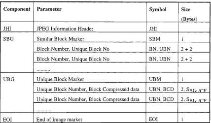
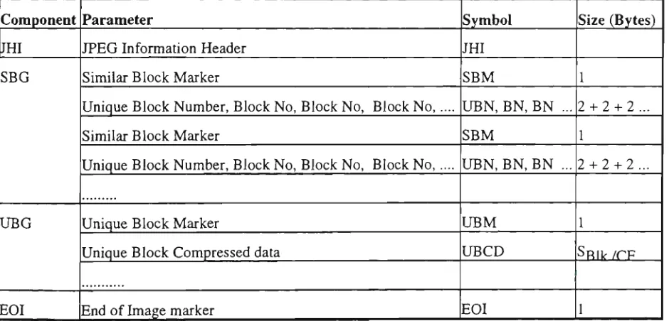
Figure 2.12 Compressed data file structure in Block Comparator Technique 33

Figure 2.13 Additional steps required in the Block Comparator Technique 37

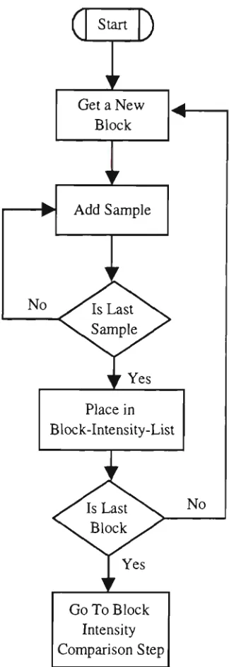
Figure 2.14 Flow chart for summation step 38

Figure 2.15 Flowchart for block intensity comparison step ,39

Figure 2.16 Selection Sort example 40

Figure 2.17 Divide and Conquer Sort example 41

Figure 2.18 Flowchart for Sample-by-Sample Comparison step 42

Figure 2.19 SIF Vs NSB for the Selection Sort method 48

Figure 2.20 SIF Vs NSB for the Divide and Conquer Sort method 48

Figure 2.21 SIF Vs NSB for the Sample-by-Sample Comparison method 48

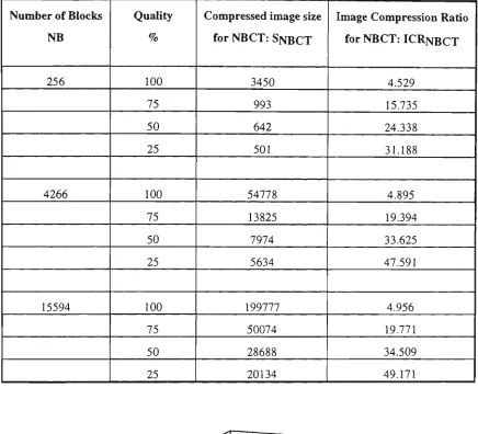
Figure 2.22 ICR Vs quality for NBCT 57

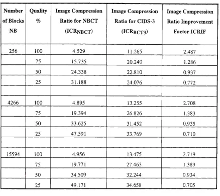
Figure 2.23 ICR Vs quality for CIDS-3 (NSB = 10%) 58

Figure 2.24 ICR Vs quality for CIDS-3 (NSB = 30%) 59

Figure 2.25 ICR Vs quality for CIDS-3 (NSB = 50%) 60

Figure 2.26 ICR Vs quality for CIDS-3 (NSB = 75%) 61

Figure 2.27 ICRIF Vs quality 62

Figure 3.2 Tree topologies 69

Figure 3.3 Mesh topologies 69

Figure 3.4 Pyramid topologies 70

Figure 3.5 Cube topology architecture 71

Figure 3.6 Classification of Image Compression Technique 72

Figure 3.7 Classification of Block Dependency 73

Figure 3.8 Classification of Image Partitioning Method 74

Figure 3.9 Classification of Memory Architecture 74

Figure 3.10 Classification of Memory Organisation / Network Topology 75

Figure 3.11 Classification of Number of Processors 75

Figure 3.12 Speedup graph 83

Figure 3.13 Speedup graph showing scaleup 83

Figure 4.1 Interconnection topology of the Mercury system 88

Figure 4.2 (T805) Transputer architecture 88

Figure 4.3 Flow diagram of implementation procedure on the Mercury system 92

Figure 4.4 Path graph for distribution and composition of image parts 92

Figure 4.5 Master and Slave units and datapaths 95

Figure 4.6 Shiva system with ParaT or NAB Slave units 95

Figure 4.7 Intel i860 processor architecture 96

Figure 4.8 Shiva system organisation 97

Figure 4.9 Rates of data transfer with respect to message size 98

Figure 4.10 Implementation procedure of the JPEG algorithm on the three processor

Shiva system 101

Figure 4.11 Task graph for three processors 102

Figure 4.12 Gantt chart of JPEG algorithm on a three transputer network 103

Figure 4.13 Param system architecture 106

Figure 4.14 Architecture of a Param 8600 node 108

Figure 4.15 i860 node architecture 108

Figure 4.16 Three nodes connection in Tree topology 109

Figure 4.17 Flow diagram of implementation procedure on the Param system 110

Figure 4.19a Graph of speedup on the Mercury system using POSIC communication

routines 113

Figure 4.19b Graph of efficiency on the Mercury system using POSIC communication

routines 113

Figure 4.20a Graph of speedup on the Mercury system using MPP communication

routines 114

Figure 4.20b Graph of efficiency on the Mercury system using MPP communication

routines 115

Figure 4.21a A comparison of speedup obtained on the Mercury system using the

POSIC and the MPP communication routines 116

Figure 4.21b A comparison of efficiency obtained on the Mercury system using the

POSIC and the MPP communication routines 116

Figure 4.22a Graph of speedup on the Shiva System 118

Figure 4.22b Graph of efficiency on the Shiva System 118

Figure 4.23a Graph of speedup on the Param system 119

Figure 4.23b Graph of efficiency on the Param system 120

Figure 4.24a Speedup graph for three parallel computers 122

Figure 4.24b Efficiency graph for three parallel computers 122

Figure 5.1 Graphical representation of Plan Pj 125

Figure 5.2a Host processor specification form 127

Figure 5.2b PE-1 specification form 127

Figure 5.3a TD-1 specification form 129

Figure 5.3b TD-2 specification form 129

Figure 5.4 SD-1 specification form 130

Figure 5.5 Module 1: "Processlmg on Host" 134

Figure 5.6 Module 2: "Processlmg on PE" 134

Figure 5.7 Module 3: "Send Complmg to SD" 135

Figure 5.8 Modules Diagram 136

Figure 5.9a Run parameter form 138

Figure 5.9b Utilisation graph of the host processor and the PE-1 at run time 138

Figure 5.10 Animation parameter specification menu 140

Figure 5.12 Time-line status graph 142

Figure 5.13 aUtilisation graph of host processor 142

Figure 5.13 bUtilisation graph of PE-1 143

Figure 5.13 c Utilisation graph of PE-2 143

Figure 5.14 SIF graph for Plans P2 and P8 151

Figure 5.15 Utilisation of TD-1 in Shared Memory Architecture 152

Figure 5.16 Utilisation of transfer devices on Distributed Memory Architecture with

Pyramid Topology 152

Figure 5.17 Speedup graph for Plans P6 and P11 for different NSB values 160

Figure A. la Speedup graph for Plan P2 A.9

Figure A.lb Efficiency graph for Plan P2 A.9

Figure A.2a Speedup graph for Plan P3 A. 10

Figure A.2b Efficiency graph for Plan P3 A.IO

Figure A.3a Speedup graph for Plan P4 A. 11

Figure A.3b Efficiency graph for Plan P4 A. 11

Figure A.4a Speedup graph for Plan P5 A.12

Figure A.4b Efficiency graph for Plan P5 A.12

Figure A.5a Speedup Graph for Plan P6 A.13

Figure A.5b Efficiency Graph for Plan P6 A.13

Figure A.6a Speedup graph for Plan P7 A.14

Figure A.6b Efficiency graph for Plan P7 A.14

Figure A.7a Speedup graph for Plan P8 A.15

Figure A.7b Efficiency graph for Plan P8 A.15

Figure A.8a Speedup graph for Plan P9 A.16

Figure A.8b Efficiency graph for Plan P9 A.16

Figure A.9a Speedup graph for Plan PI A.17

Figure A.9b Efficiency graph for Plan PI A.17

Figure A. 10a Speedup graph for Plan PI0 A. 18

Figure A. 10bEfficiency graph for Plan PIO A.18

Figure A.l la Speedup graph for Plan P l l A. 19

Figure A. l i b Efficiency graph for Plan P l l A.19

Figure A.12b Efficiency graph for Plan P12 A.20

Figure A.13a Speedup graph for Plan PI3 A.21

Figure A. 13b Efficiency graph for Plan PI3 A.21

Figure A. 14a Speedup graph for Plan P14 A.22

Figure A. 14b Efficiency graph for Plan P14 A.22

Figure A.15a Speedup graph for Plan P15 A.23

Table 4.3 Total time (Ttotal) ^ d transmission rate (R) on the SBus interface for

various message sizes 98

Table 4.4 Execution times of the JPEG algorithm on the Shiva system 104

Table 4.5 Execution times of the JPEG algorithm on the Param system 111

Table 4.6a Speedup on the Mercury system using POSIC communication routines... 112

Table 4.6b Efficiency on the Mercury system using POSIC corranunication

routines 112

Table 4.7a Speedup on the Mercury system using MPP communication routines 114

Table 4.7b Efficiency on the Mercury system using MPP communication routines ... 114

Table 4.8a The speedup comparison between POSIC and MPP communication

routines 115

Table 4.8b Efficiency comparison between POSIC and MPP communication

routines 116

Table 4.9a Speedup of the JPEG algorithm on the Shiva system 117

Table 4.9b Efficiency of the JPEG algorithm on the Shiva system 117

Table 4.10aSpeedup of the JPEG algorithm on the Param system 119

Table 4.10bEfficiency of the JPEG algorithm on the Param system 119

Table 4.11 Execution times of the JPEG algorithm on the three parallel

computers 120

Table 4.12aSpeedup of the JPEG algorithm on the three parallel computers 121

Table 4.12bEfficiency of the JPEG algorithm on the three parallel computers 121

Table 5.1 Comparison of execution times obtained from simulation and

implementation for Plan PI 141

Table 5.2 Least execution times for the NBCT Plans 149

Table 5.3 Least execution times for selected Plans using the Block Comparator

Technique 149

Table 5.4 SIF values for the NBCT Plan P2 and the BCT Plan P8 (on a Shared

Memory Architecture with Global Memory organisation ) 150

Table 5.5 SIF values for various Plans 151

Table 5.6 Least execution times for the IPC Plans Plans using the Block

Comparator Technique 152

Table 5.7 Execution times for NBCT Plan P6 and sequential block comparison

Table 5.9 Maximum speedup comparison for the NBCT Plans 157

Table 5.10 Maximum speedup comparison for the BCT Plans 158

Table 5.11 Maximum speedup comparison for the NBCT and the BCT Plans 158

Table 5.12 Speedup comparison of two architectures 159

Table 5.13 Speedup for the NBCT Plan P6 and the BCT Plan PI 1 with different

NSB 159

Table 5.14 Scaleup comparison for the NBCT Plans 161

Table 5.15 Scaleup comparison for the BCT Plans 161

Table 5.16 Scaleup comparison for the NBCT and the BCT Plans 162

Table 5.17 Scaleup comparison of two architectures 163

Table 5.18 Efficiency Cutoff Point for the NIPC Plans 164

Table 5.19 Efficiency Cutoff Point for the IPC Plans 164

Table A. 1 Execution times for NIPC Plan P2 (NBCT on a Shared Memory

Architecture with Global Memory ) A.l

Table A.2 Execution times for NIPC Plan P3 (NBCT on a Shared Memory

Architecture with Local-plus-Global Memory ) A.l

Table A.3 Execution times for NIPC Plan P4 (NBCT on a Distributed

Memory Architecture with Tree Topology) A.2

Table A.4 Execution times for NIPC Plan P5 (NBCT on a Distributed Memory

Architecture with Torus Topology) A.2

Table A.5 Execution times for NIPC Plan P6 (NBCT on a Distributed Memory

Architecture with Pyramid Topology) A.3

Table A.6 Execution times for NIPC Plan P7 (NBCT on a Distributed Memory

Architecmre with Cube Topology) A.3

Table A.7 Execution times for NIPC Plan P8 (NSB = 10%) (BCT on a Shared

Memory Architecture with Global Memory) A.4

Table A.8 Execution times for NIPC Plan P9 (NSB = 10%) (BCT on a Shared

Memory Architecture with Local-plus-Global Memory) A.4

Table A.9 Execution times for NIPC Plan PI (NSB = 10%) (BCT on a

Distributed Memory Architecture with Tree Topology) A. 5

Table A.IO Execution times for NIPC Plan PIO (NSB = 10%) (BCT on a

Table A.l 1 Execution times for NIPC Plan PI 1 (NSB = 10%) (BCT on a

Distributed Memory Architecmre with Pyramid Topology) A.5

Table A.12 Execution times for NIPC Plan P12 (NSB = 10%) (BCT on a

Distributed Memory Architecture with Cube Topology) A.6

Table A.13 Execution times for IPC Plan P13 (NSB = 10%) (BCT on a Shared

Memory Architecture with Global Memory) A.6

Table A.14 Execution times for IPC Plan P14 (NSB = 10%) (BCT on a

Distributed Memory Architecture with Torus Topology) A.6

Table A.15 Execution times for IPC Plan PI5 (NSB = 10%) (BCT on a

Distributed Memory Architecture with Pyramid Topology) A.7

Table A.16 SIF values for NBCT Plan P3 and BCT Plan P9 (on a Shared

Memory Architecture with Local-plus-Global Memory) A.7

Table A.17 SIF values for NBCT Plan P4 and BCT Plan PI (on a Distributed

Memory Architecture with Tree Topology) A.7

Table A.18 SIF values for NBCT Plan P5 and BCT Plan PIO (on a Distributed

Memory Architecture with Toms Topology) A.8

Table A.19 SIF values for NBCT Plan P6 and BCT Plan PI 1 (on a Distributed

Memory Architecture with Pyramid Topology) A.8

Table A.20 SIF values for NBCT Plan P7 and BCT Plan P12 (on a Distributed

Memory Architecture with Cube Topology) A.8

Table A.21 Speedup for NIPC Plan P2 (NBCT on a Shared Memory Architecmre

with Global Memory ) A.9

Table A.22 Speedup for NIPC Plan P3 (NBCT on a Shared Memory Architecmre

with Local-plus-Global Memory ) A.IO

Table A.23 Speedup for NIPC Plan P4 (NBCT on a Distributed Memory

Architecture with Tree Topology) A . l l

Table A.24 Speedup for NIPC Plan P5 (NBCT on a Distributed Memory

Architecture with Toms Topology) A.12

Table A.25 Speedup for NIPC Plan P6 (NBCT on a Distributed Memory

Architecture with Pyramid Topology) A.13

Table A.26 Speedup for NIPC Plan P7 (NBCT on a Distributed Memory

Architecture with Global Memory) A.15

Table A.28 Speedup for NIPC Plan P9 (NSB = 10%) (BCT on a Shared Memory

Architecture with Local-plus-Global Memory) A.16

Table A.29 Speedup for NIPC Plan PI (NSB = 10%) (BCT on a Distributed

Memory Architecture with Tree Topology) A.17

Table A.30 Speedup for NIPC Plan PIO (NSB = 10%) (BCT on a Distributed

Memory Architecture with Toms Topology) A.18

Table A.31 Speedup for NIPC Plan PI 1 (NSB = 10%) (BCT on a Distributed

Memory Architecture with Pyramid Topology) A.19

Table A.32 Speedup for NIPC Plan PI2 (NSB = 10%) (BCT on a Distributed

Memory Architecture with Cube Topology) A.20

Table A.33 Speedup for IPC Plan P13 (NSB = 10%) (BCT on a Shared Memory

Architecture with Global Memory) A.21

Table A.34 Speedup for IPC Plan P14 (NSB = 10%) (BCT on a Distributed

Memory Architecmre with Toms Topology) A.22

Table A.35 Speedup for IPC Plan P15 (NSB = 10%) (BCT on Distributed

LIST OF NOTATIONS

Notations

Description

T| Efficiency BBIP Block Based Image Partitioning BCF Block Compression Factor BCT Block Comparator Technique BD Block Dependency

BIV Block Intensity Value BN Block Number

BWIP Balanced Workload Image Partitioning CDL Component Distribution Language CIDS Compressed Image Data Stmcture DCT Discrete Cosine Transform

DCuT Distributed Memory Architecture with Cube Topology DMA Distributed Memory Architecture

DPyT Distributed Memory Architecture with Pyramid Topology DToT Distributed Memory Architecture with Toms Topology DTrT Distributed Memory Architecture with Tree Topology EIL Equal Intensity List

EOI End Of Image Marker

HMA Hybrid Memory Architecmre IBD Inter-Block Dependency ICR Image Compression Ratio

I C R B C T Image Compression Ratio for Block Comparator Technique ICRDF Image Compression Ratio Improvement Factor

ICRjsfBCT Image Compression Ratio (ICR) for Non-Block Comparator Technique

ICT Image Compression Technique used for image processing IPC Inter-Processor Communication

IPM Image Partitioning Method

JPEG Joint Photographic Experts Group MA Memory Architecture

MO Memory Organisation

MPEG Motion Photographic Experts Group MPP Message Passing Primitives

NB Number of Blocks

NBCT Non-Block Comparator Technique

NBEEL Number of blocks in Equal Intensity List

NIBD Non-Inter-Block Dependency

NIPC Non-Inter-Processors Communication NL Number of Similar Block Lists in SBG

nl Number of Block Numbers in each Unique Block list NP Number of processors

NSB Number of Similar Blocks NT Network Topology

NUB Number of Unique Blocks Px Plan-x for implementation

PI P(BCT, NIPC, BWIP, DMA, DTrT, NP) P2 P(NBCT, NIPC, BWIP, SMA, SGM, NP) P3 P(NBCT, NIPC, BWIP, SMA, SLgM, NP) P4 P(NBCT, NIPC, BWIP, DMA, DTrT, NP) P5 P(NBCT, NIPC, BWIP, DMA, DToT, NP) P6 P(NBCT, NIPC, BWIP, DMA, DPyT, NP) P7 P(NBCT, NIPC, BWIP, DMA, DCuT, NP) P8 P(BCT, NIPC, BWIP, SMA, SGM, NP) P9 P(BCT, NIPC, BWIP, SMA, SLgM, NP) PIO P(BCT, NIPC, BWIP, DMA,DToT, NP) PI 1 P(BCT, NIPC, BWIP, DMA, DPyT, NP) P12 P(BCT, NIPC, BWIP, DMA, DCuT, NP) PI3 P(BCT, IPC, BWIP, SMA, SlgM, NP) P14 P(BCT, IPC, BWIP, DMA, DToT, NP) P15 P(BCT, IPC, BWIP, DMA, DPyT, NP) PE Processing Element

POSIC Portable Operating Set of Instraction Codes RL Reference List

S Speedup for NP processors

S g c T BCT Compressed image size in Bytes

^BCTl ^ ^ ^ Compressed image size for CIDS-1 in Bytes SBG Similar Block Group

SBlk

S B N F

^Comoime SD

S E O I

SIF

SJHI SLgM

SGM SMA

S N B C T

SOF SOI SOS SSBM ^Srcime SUBM SUBNF Tl

T B C

TCS

TD

T D C T

Tdct ^Enco ^Intcomn TjPEG T N ^Ouan ^samoblock

Size of one block in Bytes Size of the Block Number Field Compressed image data size in Bytes Storage Device

Size of End Of Image marker Speed Improvement Factor

Size of JPEG Header Information in Bytes

Shared Memory Architecture with Local-Plus-Global Memory organisation

Shared Memory Architecture with Global Memory organisation Shared Memory Architecture

NBCT Compressed image size in Bytes Start Of Frame

Start Of Image marker Start Of Scan

Size of the Similar Block Marker Source image data size in Bytes Size of the Unique Block Marker

Size of the Unique Block Number Field Time taken by a single processor

Total number of Base Operations required for Block Comparison Total number of Base operations required for subtraction operation for one 8 x 8 block

Transfer Device

Total number of Base Operations required for DCT step for one 8 X 8 block

Total number of Base operations required for DCT function for one 8 x 8 block

Total number of Base Operations required for Huffman Encoding for one block

Total number of Base Operations for block intensity value comparison

Total number of Base Operations taken by the JPEG algorithm Time taken by N processors

Total number of Base Operations required for Quantisation step for one 8 x 8 block

samocomo

samosum

T

T

^sum

UBG

UBFV

UBN

VQ

Total number of Base Operations for comparing samples of a

block with those of existing Unique Blocks

Total number of Base Operations required for the summation of

sample values in any image block

Total number of Base Operations for summation of samples in all

image blocks

Unique Block Group

Unique Block Intensity Value

Unique Block Number

Chapter 1

INTRODUCTION

Contents

1.1 Introduction 2

1.2 Problem Statement 2 1.3 Literature Re view 3 1.4 Research Objectives 7 1.5 Thesis Outline 8

Abstract

This chapter gives an introduction to the existing digital image compression techniques, parallel processing techniques, the research problem and investigation procedures described in this thesis.

1.1 Introduction

Digital image compression is used to reduce the number of bits required to store an image in computer memory and/or transmit it over a communication link [Jain, 89]. Image compression prior to transmission should reduce the amount of information to be transmitted, thus lowering the bandwidth requirements and cost. The main focus of this research is to enhance the performance of the current digital image compression method. Details of the research problem are given in section 1.2.

A literature review of existing digital image compression standards, and techniques to improve compression parameters such as quality, speedup and compression ratio are discussed in section 1.3.

Research objectives are explained in section 1.4. Outline of thesis chapters is given in section 1.5.

1.2 Problem Statement

Transmission of image data using simple techniques requires a bit rate that is too large for many communications links or storage devices. Digitisation may be desirable for security and/or reliability, but it can cause bandwidth explosion. Hence data compression is required to use the available bandwidth as effectively as possible.

Over the past decade advancements in technology have spawned many applications of digital imaging, such as photo videotex, desktop publishing, graphics arts, colour facsimile, newspaper wirephoto transmission, medical imaging. For many other contemporary applications, such as distributed multimedia systems rapid transmission of images is necessary. Images are used in multimedia for browsing, retrieval, storage and slide show. Research challenge includes developing real-time compression algorithms and guaranteed Quality of Service in multimedia applications [Furht, 94] [Furht, 95]. Dollar cost as well as time cost of transmission and storage tend to be directly proportional to the volume of data. Therefore, application of digital image compression techniques become necessary to minimise these costs.

the JPEG algorithm and a study of techniques for parallel implementation of image compression is presented.

1.3 Literature Review

Literature survey covered similar work reported in journals and conference proceedings. To provide an overview of previous work and to provide a basic theoretical understanding of the subject, the papers presented by various authors are reviewed and quoted in this chapter. The areas covered in the literature survey are: digital image compression techniques, standards such as JPEG, MPEG, PX64, parallel implementations, performance analysis issues.

Digital image compression techniques are discussed in section 1.3.1. Image compression algorithms include optimisation of parameters, such as quality, complexity, compression ratio and speedup of operation. Techniques employed to improve these parameters are discussed in section 1.3.2.

L3.1 Digital Image Compression Techniques

Various digital image compression techniques, hardware, and software are discussed in this section.

Digital image compression techniques can also be classified based on the algorithms used such as Wavelet transform. Fractal image, Vector Quantisation and DCT. The Wavelet transform algorithm is based on basis functions [Koomwinder, 93]. Fractal images are based on Iterated Function Systems (IFS) [Bamsley, 93]. Vector Quantisation is based on vector representation of the image and based on code book design [Cosman, 96] [Gersho, 92]. The JPEG algorithm is based on Differential Pulse Code Modulation (DPCM) and the DCT [Pennebaker, 93].

Wavelet transform can also be used with the JPEG standard in the video industry for on-line editing [Cornell, 93]. The VQ method is complicated by the need for code design. Therefore, coding with Vector Quantisation is slow as compared to coding with the JPEG algorithm. VQ is more efficient when it is combined with other techniques. The JPEG standard is widely used for still imaging applications. The JPEG algorithm is used in the standard developed by the Motion Pictures Expert Group (MPEG), for compressing moving pictures as well. Therefore, the JPEG algorithm was chosen for this research purpose.

Aravind has described a number of digital image compression algorithms and standards, such as the JPEG, the MPEG and PX64 [Aravind, 89]. The JPEG standard is described in sufficient detail in [Nelson, 92a], [Pennebaker, 93] and [Wallace, 92]. A very succinct description of the various techniques used in the JPEG standard is given by William Pennebaker in [Pennebaker, 93]. The MPEG standard is described in [Gall, 91] and [Draft, 90]. The PX64 compression algorithm for video telecommunications is described in [Liou, 91]. PX64 algorithm consists of DCT-based intraframe compression, which is similar to JPEG algorithm and predictive interframe coding based on Differential Pulse Code Modulation (DPCM) and motion estimation. Therefore all these standards use the DCT-based method of compression as a basic step.

Two prominent image compression techniques are predictive technique and DCT-based technique [Pennebaker, 93]. The JPEG was working on still image compression using both techniques. The predictive technique is a lossless compression technique while the DCT - based technique is a lossy technique. The DCT-based method of compression is widely used, as it is suitable for a large number of applications, and also, it is expected that DCT-based technique developed for implementing the JPEG standard can be applied to compressing motion picmres as well; because the MPEG standard is also based on the DCT .

1.3.2 Performance Improvement

In developing digital coders many parameters need to be considered, such as bit rate, quality of output image, complexity of the algorithm, compression ratio, quality of service and speed of operation. Reduced bit rate reduces quality, unless complexity of the coding technique is increased. Complexity raises cost, and in many coding techniques it increases the processing delay as well.

The JPEG algorithm compresses the image based upon a user specified quality factor, where for higher quality of output image lower compression ratio can be achieved and vice verse. In the JPEG compressed data structure block numbers are not specified. If any block is lost during transmission then the output image is not the same as the input image.

Papathanassiadis T. [Papathanassiadis, 92] discussed compressed image data structure with block numbers. This has the potential of improving the quality of service. But, by including block numbers the compression ratio gets reduced.

Roberto Rinaldo [Rinaldo, 95] has discussed block matching technique for fractal image coding technique. The proposed coding scheme consists of predicting blocks in one subimage from blocks in lower resolution subbands with the same orientation. This block prediction scheme is simpler than the iterative scheme adopted in standard fractal block coders and visual quality is better than the other schemes. A drawback of Rinold's scheme is the larger encoding time required in comparison to the time required in coding techniques like JPEG.

The DCT-based methods work on each block of image independently, therefore, the JPEG algorithm can be parallelised by processing each image block on a separate processor. The JPEG algorithm can thus be implemented on parallel computer architectures.

Rapid advances in electronics technology throughout the 1980s has allowed more complex, yet relatively inexpensive computational devices with greatly increased throughput to be developed. New concurrent (or parallel) techniques using fast sequential processing devices, and multi-processing devices are now being applied to digital data compression. Existing parallel implementations of digital image compression are discussed below.

Therefore, on the 64 node MEiKO or the iPSC/2 computers compression algorithm could not achieve real-time compression. Even if the number of processors is increased in the iPSC/2 computer, the minimum compression time that could be obtained is nearly 2 sec/fi-ame [Tmker, 89].

Compact Disc-Interactive (CD-I) fliU motion video encoding algorithm was implemented on Parallel Object Oriented Machine (POOMA). This system was developed at the Philips research laboratories. It is based on the Motorola MC68020 with a loosely coupled MIMD architecture and consists of 100 nodes. Compression algorithm took less than 2 sec/fi-ame on 100-processor nodes [Sijstermans, 91]. For the parallel algorithm used, saturation will occur if more than 100 processors are used. Thus, for real-time applications even this system is not quite adequate.

The HDTV Codec is based on a motion-adaptive DCT algorithm. It consists of a parallel signal processing architecture and LSI gate array [Kinoshita, 92]. This hardware compresses the motion picture at the bit rate of 130 Mb/s, that is, in real-time. This hardware is specific to motion image compression.

S. Srinivasan [Srinivasan, 93] describes the design of a real time image processing system using DSP 56000/96000 family of processors. This system can be used for a variety of image processing and graphic applications which require transform computations. However, it is found that the system is not very eflBcient for coding and decoding part of the image compression algorithm.

John Elliott [Elliott, 89] describes simulation of image compression algorithm on a supercomputer based on the Transputer processor along with the architecture of the Edinberg Concurrent supercomputer. The parallel algorithm used on this supercomputer can process 6 - 7 frames/sec by optimising the code. But for real-time image compression a speed of at least 18-20 fi-ames /sec is required.

M. N. Chong [Chong, 90] describes implementation of the adaptive transform coding technique on a transputer based quadtree architecture. There is a limitation to the degree of parallelism that can be achieved in this implementation. The results obtained on the quadtree structure for various sized networks are given in this paper. The least execution time of 1.538 sec. is obtained on 16 processors. This execution time is higher than that required for real-time image compression.

R. Aravind [Aravind, 89] explains implementation of the DCT-based JPEG decompression algorithm on a Digital Signal Processor (DSP)-based system. This decoder is capable of processing in real-time, at approximately 15 fi-ames/sec with a fi-ame size of 128 x 96.

architecture for a 256 x 256 pixel monochrome still image. The execution time varies

firom 0.61 sec. to 0.12 sec as the number of processors is increased firom one to six. For

a large image size, image compression can be achieved in close to real-time by increasing

the number of DSP processors in the network.

Peter Monnes and Borko Furht [Monnes, 94] explain analysis of parallel JPEG

algorithm on Intel i80286 and i80386 processors. The parallel technique used in this

paper uses parallelisation only for DCT and quantisation part of the JPEG algorithm. The

encoding part is done serially. Therefore there is still opportunity for parallelisation of

JPEG algorithm.

Placement of blocks of image data on different parallel architectures is one of the

many issues that was explored and investigated fiirther. Papathanassiadis T.

[Papathanassiadis, 92] discussed various image partitioning strategies. There are two

main methods used for image partitioning: with interblock dependency and without

interblock dependency. Chung-Ta King [Chung-Ta King, 91] discussed strategies for

partitioning and processing images with interblock dependency on distributed memory

multi-computers. Browne [Browne, 89] discussed the various options of image

processing mapping methods onto Transputer networks.

1.4 Research Objectives

JPEG is one of the most widely used image compression standard. This research is

focused on improving the performance of this standard, and its implementation on

parallel architectures. Hardware (VLSI chips) which implement the JPEG image

compression algorithm are available. Such hardware is specific to image compression

only and can not be used for other image processing applications. A flexible means of

implementing digital image compression algorithms is still required. An obvious method

of processing different imaging applications on general purpose hardware platforms is to

develop software implementations.

enhancing the current JPEG standard is investigated, to reduce the compressed image size and to improve the speed of compression.

One of the primary objectives of this research project was to develop techniques for exploitmg parallel processing systems for real-time image compression and decompression. It is expected that such parallel processing technique will not only reduce the execution time, but will also accomplish other significant performance improvements such as improved quality of compressed image, improved reliability and availability of the system, and better scalability. Therefore various options are investigated for implementing digital image compression algorithms on parallel architectures.

Some of the implementation options were studied by simulating these on computer models. A simulation package called NETWORK n.5 was used for building the computer model and running the required experiments on the same. Simulation results were used to determine speedup, scaleup and efficiency of the techniques developed.

1.5 Thesis Outline

This section gives a brief description of each of the following chapters.

Chapter 2 Digital image compression techniques: In this chapter different digital

image compression techniques, and the JPEG image compression standard are described. Digital image compression techniques are based on algorithms such as Wavelet transform, Fractal images, Vector Quantisation and Discrete Cosine Transform. Digital image compression technique developed by the Joint Photographic Experts Group is based on the Discrete Cosine Transform.

The JPEG technique is applicable to a wide variety of applications and is one of the most widely used technique. Therefore, JPEG technique is chosen as the main focus for our research. Present JPEG compression process is done block-by-block in a sequential manner. An enhancement to the current JPEG compression technique is proposed, to speedup the operation and reduce the compressed image size.

Chapter 3 Parallel processing plans for digital image compression techniques: This

Digital image compression can be performed on parallel computers in a variety of ways. Each uniquely identifiable way of implementation is called a Plan. Each Plan can be specified as a 6-tuple consisting of image compression technique, block dependency, image partitioning method, memory architecture, network topology and the number of processors. Some of these Plans were implemented on available parallel computers and other Plans were simulated using the Network n.5 simulation package.

Model building and simulation involves ten steps, viz. problem formulation, model building, data collection, model translation, model verification, model validation, experiment planning, experimentation, analysis of results, and documentation. Each of these steps are described briefly in this chapter.

Chapter 4 Implementation of the JPEG algorithm on parallel computers: This

chapter describes the hardware architecture and methods used for the implementation of the JPEG algorithm on parallel computer systems such as Mercury, Shiva and Param. The Mercury system has a distributed memory architecture. Shiva system has a shared memory architecture, and the Param system uses hybrid memory architecture.

JPEG algorithm was implemented on these three parallel computers with different image sizes and on various sized networks. This chapter describes implementation of the JPEG algorithm on three parallel computer systems and it gives the experimental results obtained on the same.

Chapter 5 Simulation of digital image compression techniques: This chapter

describes modelling and simulation methods used for investigating parallel processing of image compression techniques, using the Network II.5 simulation package. Image compression Plans have been modelled for different parallel computer architectures using the Network II. 5 simulation package. This chapter describes details of the model building process and the process of running simulation experiments for various Plans. Simulation results for these Plans are compiled to evaluate the performance of these Plans.

Speedup, scaleup and efficiency obtained for each Plan is given and the performance of different Plans are compared.

Chapter 6 Conclusions and future research: This chapter gives the conclusions and

Chapter 2

DIGITAL IMAGE COMPRESSION TECHNIQUES

Contents

2.1 Introduction U 2.2 Digital Image Compression Techniques 11

2.3 JPEG Standard 15 2.4 Block Comparator Enhancement to the JPEG Algorithm 29

2.5 Summary 63

Abstract

This chapter describes digital image compression techniques, and the JPEG image compression standard. Digital image compression techniques are based on algorithms such as the Wavelet transform. Fractal images. Vector Quantisation and Discrete Cosine Transform (DCT). The digital image compression technique developed by the Joint Photographic Experts Group (JPEG) is mainly based on the quantisation of the DCT.

The JPEG technique is applicable to a wide variety of applications and is one of the most widely used technique. Therefore, the JPEG technique is chosen as the main focus for this research. Presently, JPEG compression process is done block by block in a sequential manner. An enhancement to the current JPEG compression technique is proposed. The aim of this enhancement is to speedup the operation and reduce the compressed image size.

2.1 Introduction

Digital image compression techniques can be broadly classified into still image

compression and motion image compression techniques. Still image compression

techniques can be fiirther classified based on the algorithm used for compressing the

image such as Wavelet transform. Fractal images. Vector Quantisation (VQ) and the

Discrete Cosine Transform (DCT). These digital hnage compression algorithms are

described in section 2.2.

The JPEG standard is widely used for still imaging appUcations. The JPEG

algorithm is used in the standard developed by the Motion Pictures Expert Group

(MPEG), for compressing moving pictures as well. Therefore, The JPEG algorithm was

chosen for our research. Section 2.3 describes the JPEG algorithm in detail.

JPEG uses an 8 x 8 block of image samples as the basic element for compression.

These blocks are processed sequentially. There is always a possibility of having similar

blocks in a given image. If similar blocks are located in an image, then repeated

compression of these blocks is not necessary. By locating similar blocks in an image,

speed of compression can be increased and the size of compressed image can be reduced.

The technique used to enhance the JPEG algorithm is called Block Comparator

Technique in this thesis. This Block Comparator Technique (BCT) is described in section

2.4.

2.2 Digital Image Compression Techniques

By using mathematical methods such as Fourier transform, it is possible to represent a

given image in terms of a few basis fiinctions [Hunt, 93]. Recently, mathematicians,

scientists and engineers have been active in seeking new methods for representing signals

or data in terms of basis fijnctions. Because these fijnctions can be analysed, understood

and characterised in a succinct maimer, these methods can be applied to digital image

compression and many other applications.

technique include the Joint Bi-level Image Experts Group (JBIG) algorithm and the JPEG algorithm (predictive technique) [Pennebaker, 93]. Lossy compression techniques are used in applications such as colour facsimile, newspaper wire-photo transmission, medical imaging, graphics arts, photovideotex, desktop publishing, and many other still imaging applications.

Digital Image Compression Techniques

Lossless Compression Technique Lossy Compression Technique

JPEG (Predictive J B I G JPEG (DCT-based Fractal VQ DCT

Technique) Technique) Wavelet

Figure 2.1 Digital image compression techniques

The Wavelet transform algorithm is based on basis fiinctions; these are described in section 2.2.1. Fractal images are based on Iterated Function Systems (IFS); these are described in section 2.2.2. Vector Quantisation is based on vector representation of the image and code book design; this is described in section 2.2.3. The JPEG algorithm is based on the DCT and Differential Pulse Code Modulation (DPCM). The DCT-based method is described in section 2.2.4.

2.2.1 Wavelet Transform

There are two types of Wavelet Transforms ie. Continuous Wavelet Transform and Discrete Wavelet Transform. The Continuous Wavelet Transform was first presented by Grossmann and Morlet in 1984. Thereafi;er it was developed by others, including Holschneider (1988), Ameo'odo et al. (1989), Forge (1992). Daubechies (1986 and 88) was one of the first to work on Discrete Wavelet Transform. Wavelet transformation has a number of applications in signal processing and data compression.

Wavelet basis functions are orthonormal. Therefore, these transformations can be used to remove redundant signals from the original signal, this leads to compression of the original signal.

In Wavelet compression the original multi-resolution image is decomposed into a low resolution signal and a difference signal [Nacken, 93] [Koomwinder, 93]. The low resolution signal is an average of the low frequency signals and is calculated by applying low pass filtering, followed by subsampling. The low resolution signal can be described by a smaller number of samples than the original image. The difference signal is the difference between the low resolution image and the actual image. The difference signal can be coded with a smaller number of bits per pixel. Thus the total number of bits required to encode the image is smaller than the original image.

2.2.2 Fractal Image Compression

Fractal image compression is based on Iterated Function System (IFS) theory and the Collage theorem. Fractal image compression can be achieved via the IFS compression algorithm, which is an interactive image modelling method based on the Collage theorem.

IFS fractals can be obtained through suitable transformation of the image [Bamsley, 93]. Such fractals can be used as approximates for real world images. Real world image is one of many basic shapes, such as a leaf or a letter of the alphabet, or a black and white fem, or a black cat sitting in a field of snow, etc. These fractals have the property that they are themselves models for real world images, and at the same time can be defined by finite strings of zeros and ones. This makes them suitable for image compression.

The Collage theorem says that "to find an IFS whose attractor is close to looks like a given set, one must try to find a set of transformations, contraction mappings on a suitable space within which the given set lies, such that the union, or collage, of the images of the given set under the transformations is close to or looks like the given set" [Bamsley, 93]. The degree to which two images look alike is measured using the Hausdorff metric.

2.2.3 Vector Quantisation

one of a stored set of templates or codewords. In this way the complicated image signal can be replaced by a series of simple table lookups.

The following theorem shows that VQ can at least match the performance of any arbitrarily given coding system that operates on a vector of signal samples or parameters. Theorem is as follows. " For any given coding system that maps a signal vector into one of N binary words and reconstructs the approximate vector from the binary word, there exists a vector quantiser with codebook size N that gives exactly the same performance, ie. for any input vector it produces the same reproduction as the given coding system" [Gersho, 92].

Pattem matching with set of codebooks is done in several ways, such as nearest neighbour quantiser and exhaustic search algorithm [Gersho, 92]. In the nearest neighbour quantiser search algorithm, a vector is represented by the nearest vector stored in the codebook. An advantage of such an encoder is that the encoding process does not require any explicit storage of the geometrical description of the cells. In exhaustic search algorithm, the search is performed sequentially on every code vector in the codebook, keeping track of the "best so far" and continuing until every code vector was tested. This method of pattem matching requires more time but the resulting compression is better than the nearest neighbour quantiser method.

2.2.4 Discrete Cosine Transform

Discrete Cosine Transform is widely used for many digital image compression techniques. Digital image compression technique developed by the Joint Photographic Experts Group (JPEG) is based on the DCT and predictive algorithm. The Consultative Committee for Intemational Telegraph and Telephone (CCITT, now called Intemational Telephone Union - ITU) and Intemational Standard Organisation (ISO) formed this committee to develop compression standards for still and motion pictures [Wallace, 92].

In the JPEG algorithm there are mainly two image compression methods viz. predictive method which is carried out in the spatial (data) domain, and the transform method which is performed in the frequency domain [Leger, 91]. The predictive method is a lossless compression technique while the DCT-based method is a lossy compression technique. DCT-based method of compression is widely used as it is easier to implement and is suitable for a large number of applications including motion picmre compression.

algorithm is added to support TIFF file reading and writing facilities [Cockroft, 91]. JPEG is also used for Picmre Archiving and Communication Systems (PACS) in medical imaging field [Kajiwara, 92]. A detail description of the JPEG standard is given in the next section.

2.3 JPEG Standard

There are three intemational standards available for image compression for different applications, viz. JPEG, MPEG, and P*64 [Quinnell, 93]. JPEG is intended for continuous-tone still images, MPEG is intended for video images, and P*64 is for video telephony. In this section the JPEG standard is described.

The first step in the JPEG algorithm is to locate data redundancy in the image pixel values. This is done by using the Discrete Cosine Transform, which is similar to the Fourier Transform but includes only the Cosine part of the function. Wavelet transforms can also be used with the JPEG standard in the video industry for on-line editing [Comell, 93]. The Vector Quantisation (VQ) method is complicated by the need for code design. Therefore, coding with Vector Quantisation is slow as compared to coding with the JPEG algorithm. Vector Quantisation is more efficient when it is combined with other techniques. Therefore, the JPEG algorithm was chosen for our research purpose. The JPEG algorithm can be implemented in hardware as well as in software [Baran, 90].

Details of the DCT-based JPEG algorithm are given in section 2.3.1. The available hardware chips in VLSI implementation include the C-Cube Micro system's CL550 chipset, the SGS-Thomson's STl 140 CMOS chip [Leonard, 91], and Intel's Digital Video Interactive (DVI) chip [Vaaben, 91]. Section 2.3.2 describes the CL550 chip in brief.

JPEG has developed software implementation that can be used on general purpose machines and can be modified easily according to the application requirement. Section 2.3.3 describes the version-4 of modified JPEG software.

JPEG compressed file stmcture is described in section 2.3.4.

2.3.1 DCT-Based JPEG Algorithm

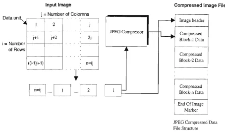
YUV ( Y for luminance or brightness, U and V for colour difference signals R and Y-B respectively), Cyan Magenta Yellow and Y-Black (CMYK) [Ang, 91]. Each component consists of a rectangular array of samples. A sample is defined to be an unsigned integer with the range [0, 2? -1] or signed integer with the range [-2? , 2?-!], where p is sample precision in bits. The JPEG standard has defined the concept of a "data unit". A data unit is an 8 x 8 block of samples in DCT-based codecs. Generally, data units of image components are ordered from left-to-right and top-to-bottom.

Components of an image can be stored in one of two possible formats, namely interleaved format and non-interleaved format. If an image component is stored in the non-interleaved format, the data units are ordered in a pure raster scan sequence as shown in figure 2.2.

Top

IL . - . . _ . _ _ . _ _ . .^Data Units

Left

Right

Bottom

Figure 2.2 Non-interleaved data ordering

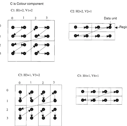
If the image has two or more colour components each one of these may be stored in an interleaved format. Each component Ci is partitioned into rectangular regions of Hi X Vi data units, as shown in the generalised example of figure 2.3. Regions within a component are ordered from left-to-right and top-to-bottom. Within a region also, data units are ordered from left-to-right and top-to-bottom.

2,3.1.1 DCT-based Compression Steps

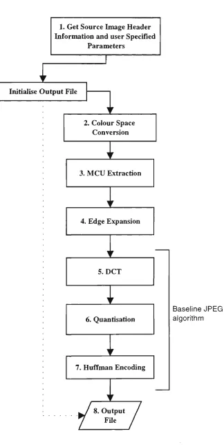
Modified JPEG algorithm involves colour space conversion. Minimum Coded Unit (MCU) extraction, DCT, quantisation and encoding steps as shown in figure 2.4. Each of these step are described below.

2. Conversion from input image format to a standard internal format (either RGB or grayscale). Colour space conversion (eg. RGB to YCbCr). This is a null step for grayscale images.

1

2

3

C is Colour component C1:H1=2,V1=2

0 1 2 3

Z^

r^l

^ ^

"y:

C2: H2=2, V2=l

Data unit

^—Region

C3: H3=1,V3=2

0 1 2 3

Vl±1.

rWi

C4: H4=l, V4=l

o—^o—^o^^^o

Figure 2.3 Interleaved image data ordering

The following steps (3 to 8) are performed once for each scan of a complete image, i.e. once if making a non-interleaved file, and more than once for an interleaved file.

3. Minimum Coded Unit (MCU) extraction, i.e. creation of a single sequence of 8 x 8 sample blocks.

4. Edge expansion. This step operates independently on each colour component. 5. DCT transformation of each 8 x 8 block.

6. Quantisation, scaling and zigzag reordering of the elements in each 8 x 8 block. 7. Huffman (or arithmetic) encoding of the transformed block sequence.

1. Get Source Image Header Information and user Specified

Parameters

L

Initialise Output File

1

Conversion

I

3. MCU Extraction

I

HZ-n

I

6. Quantisation

I

7. Huffman Encoding

/

rr^

Baseline JPEG algorithm

8. Output File

2.3.1.1a Input File and Parameters

The input image file to be compressed by the JPEG algorithm can be in either of the following formats: PPM (Pulse Pixel Map), GIF (Graphics Literchange Format), RLE (provided by Utah Raster Toolkit). Details of these formats differ but the type of information included in each of these is similar. In general, an input file contains information about the format used, image width, image height, maximum value of the sample, and the image data.

Parameters such as quality factor, smoothing factor, and sampling ratio are input by the user. For any unspecified parameters the default value is used by the software.

Quantisation tables are generated by taking into account the specified quality factor. AC and DC Huffman tables are also generated as part of the algorithm execution. Currently, the values generated are fixed by the JPEG standard. Though, it is possible to vary these tables to get compressed images of different compression ratios. The output file includes appropriate header along with the quantisation tables and Huffman tables. The subsequent step, colour space conversion, is explained in the next section.

2.3.1.1b Colour Space Conversion

The JPEG source image is divided into groups of rows. The number of rows in each group is equal to the maximum sampling factor. Each source image group (GrpSrcImg) is subjected to Colour Space Conversion (ClrSpcCnv) step. This step converts the input colour space of any format to the YCbCr format. The YCbCr format is defined by the CCIR 601-1 standard. For example, if the input image is in the RGB colour format, then the values of the Y, Cb, and Cr components can be calculated by the following formulae:

Y = 0.299900 * R + 0.58700 * G + 0.11400 * B

Cb = -0.016874 * R - 0.33126 * G + 0.50000 * B + MAXJSAMPLE/2 Cr = 0.50000 * R - 0.41869 * G - 0.08131 * B + MAXJS AMPLE/2.

Here MAXJSAMPLE is maximum value of sample in a source image. For example, in an 8-bit image, MAXJSAMPLE is 255.

2.3.1.Ic MCU Extraction

The JPEG proposal defines the term "data unit" as a block of 8 x 8 samples and MCU to be the smallest group of interleaved data units. MCU extraction is used for better organisation of data units for interleaved image data. MCU is a group of data units taken from the same region of all image components.

A maximum of four components can be interleaved. And a maximum of ten data units are allowed in an MCU. Because of this restriction, not every combination of four components which can be represented in non-interleaved order within JPEG compressed image is allowed to be interleaved. The JPEG proposal allows some components to be interleaved and some to be non-interleaved within the same compressed image.

In the JPEG algorithm, the blocks of 8 x 8 samples and image components are processed sequentially; even though it is also possible to process image components simultaneously. In the non-interleaved format image components are independent of each other; whereas, in the interleaved format image components are dependent upon each other. In the interleaved format a maximum of four image components can be used in a single MCU. Thus, up to four image components can be processed at a time.

2.3.1.Id Edge Expansion

Edge expansion is used to make the number of samples in a block, a multiple of the MCU dimension. This is done by duplicating the right-most column and/or bottom-most row of pixels.

2.3.Lie Discrete Cosine Transform (DCT)

The Discrete Cosine Transform (DCT) is calculated for each block of the MCU. Output of the DCT F(u, v) gives orthogonal basis signals given by

F(u.v) = 1 C(u)C(v)[ I i f ( x , y ) * c o s - ( 2 ^ * c o s - ( ? ^ ] (2.1) 4 x=Oy=0 ^^ ^°

where C(u), C(v) J = l / V 2 u,v = 0

[= 1 otherwise,

and F(u,v) = Discrete cosine transformed signal.

2.3.1. If Quantisation

Quantisation is achieved by dividing each DCT coefficient by its corresponding quantiser step size and rounding off to the nearest integer value, so that

Quantised value Q(u,v) = Integer Round ( DCT coefficient / Quantiser step size). (2.2)

Quantiser step size is calculated with respect to the desired quality of the output image. This step is performed to achieve compression by representing DCT coefficients with no greater precision than is necessary to achieve a desired image quality. On performing quantisation, visually insignificant values are discarded.

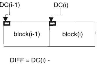
2.3.1.Ig Huffman Encoding

The first value to be encoded in a block is the DC coefficient. This DC coefficient is encoded.as the difference between the DC term of this block and that of the previous block, in the encoding order shown in figure 2.5.

DC(i-1) DC(i)

DIFF = DC(i)

-Figure 2.5 Encoding the DC coefficient