Do light nuclei display a universal γ-ray strength function?

Do light nuclei display a universal

γ

-ray strength function?

M. Guttormsen1,a, A.C. Larsen1, A. B¨urger1, A. G¨orgen1, H.T. Nyhus1, S. Siem1, N.U.H. Syed1, H.K. Toft1_{, G.M. Tveten}1_{, S. Harissopulos}2_{, T. Konstantinopoulos}2_{, A. Lagoyannis}2_{, G. Perdikakis}2_, A. Spyrou2_{, M. Kmiecik}3_{, K. Mazurek}3_{, M. Krti˘cka}4_{, T. L¨onnroth}5_{, M. Norrby}5_{, A. Schiller}6_{, and} A. Voinov6

1 _{Department of Physics, University of Oslo, N-0316 Oslo, Norway} 2 _{Institute of Nuclear Physics, NCSR ”Demokritos”, Athens, Greece} 3 _{Institute of Nuclear Physics PAN, Krak´ow, Poland}

4 _{Institute of Particle and Nuclear Physics, Charles University, Prague, Czech Republic} 5 _{Department of Physics, Åbo Akademi University, FIN-20500 Åbo, Finland}

6 _{Department of Physics and Astronomy, Ohio University, Athens, Ohio 45701, USA}

Abstract. In this work we focus on properties in the quasi-continuum of light nuclei. Generally, both level density andγ-ray strength function (γ-SF) differ from nucleus to nucleus. In order to investigate this closer, we have performed particle-γcoincidences using the reactions (p,p0

), (p,d) and (p,t) on a46_{Ti target. In particular, the very rich data} set of the46_Ti(p,p0

)46_{Ti inelastic scattering reaction allows analysis of the coincidence} data for many independent data sets. Using the Oslo method, we find one common level density for all data sets. If transitions to well-separated low-energy levels are included, the deducedγ-SF may change by a factor of 2−3, due strong to Porter-Thomas fluctuations. However, a universalγ-SF with small fluctuations is found provided that only excitation energies above 3 MeV are taken into account. The nuclear structure of the titaniums is discussed within a combinatorial quasi-particle model, showing that only few Nilsson orbitals participate in building up the level density for these light nuclei.

1 Introduction

The Oslo group has studied the low-energy tail of the giant electric dipole resonance (GEDR) in vari-ous mass regions. The method is based on measuring particle-γcoincidences from light-ion reactions with only one charged ejectile. In this way theγ-ray emission can be studied as function of excitation energy up to the particle separation energy. In the framework of the Oslo method, these spectra can be used to simultaneously extract level density andγ-ray strength function (γ-SF).

Many experimental groups have extensively studied the smooth behavior of the GEDR [1]. For heavy nuclei far away from closed shell, the various statistical gross properties vary slowly from nucleus to nucleus, see e.g. [2]. The Oslo group has particularly studied the low-energy tail of the GEDR for rare-earth nuclei. Here, theγ-SF is found to be nicely fitted by the KMF-model [3] with a superimposed Lorentzian originating from the strength of theM1-scissors mode1_{. Thus, one may claim} that theγ-decay of these nuclei is governed by an underlyingγ-SF that is experimentally observable. Figure 1 demonstrates the smooth behavior of theγ-SF in171Yb.

The level densities are also very similar for neighboring rare earth nuclei, however, there is a pronounced odd-even mass effect. An odd-mass nucleus, say171Yb, has 5−7 times more levels than

a _{e-mail:[email protected]}

1 _{Typical resonance parameters of the scissor mode in deformed reare earth nuclei are:E}

γ∼3 MeV, σEγ ∼1 MeV andB(M1)∼6µ2N.

Fig. 1.A pygmy resonance found in171_{Yb observed for two different reactions [2]. The solid line in the upper} panels is a fit to data including all contributions. The dashed lines are due to the KMF-modeled tail of the GEDR. The difference between the totalγ-SF data and the KMF-model is shown in the lower panels.

its even-even neighbors170_{Yb and}172_{Yb. This is due to the fact that nucleons not coupled in Cooper} pairs [4], may populate various unoccupied single-particle orbitals and thus contribute significantly to the total level density.

The smooth behavior vanishes for lighter nuclei, typically for nuclei with mass numbersA<60. It may look like each nucleus has its ownγ-SF and that the function even depends on excitation energy. In a recent study [5] theγdecay has been simulated for a light nucleus resembling57_{Fe. The level} density andγ-SF entering the simulated data are known. It turns out that the Oslo method reproduces the level density, but not the true inputγ-SF. The expectedγ-decay pattern may be hidden for several reasons related to:

– Low level density – Irregular spin distribution – Asymmetric parity distribution

Thus, the nucleus may not have available states with right spin and parity to reveal the fully allowed γ-SF.

In this work we will search for a universalγ-SF in the titanium mass region. In particular the 46_Ti(p,p0₎46_{Ti reaction gives a very rich data set that allows to compare severalγ-SFs at different}

(keV) γ E

2000 4000 6000 8000 10000 12000

E (keV)

0 2000 4000 6000 8000 10000

1 10

2 10

3 10

1 10

2 10

3 10

Primary gammas

Fig. 2.The first-generationγ-ray matrix of46_{Ti obtained from the inelastic proton reaction. Only a part of the}

P(E,Eγ) matrix is utilized, namely data withEγ>1.8 MeV and 5.5<E<10 MeV.

2 Experiments

The experiments were conducted at Oslo Cyclotron Laboratory (OCL) using 15 and 32 MeV proton beams on a self-supporting target of46Ti. The thickness of the target was 1.8 mg/cm2. The reactions studied are 46Ti(p,p0)46Ti,46Ti(p,d)45Ti and46Ti(p,t)45Ti, which have been reported in [6–8]. The charged ejectiles are used to tag the excitation energies for eachγ-ray spectrum from the ground state and up to the neutron separation energy.

The particle-γcoincidences are measured with the efficient CACTUS multi-detector array [9]. The coincidence set-up consists of eight collimated∆E – E type Si particle telescopes, placed at a distance of 5 cm from the target and making an angle ofθ=45◦with the beam line. The particle telescopes are surrounded by 28 5”×5”NaIγ-ray detectors, which have a total efficiency of∼15% of 4π.

The experimental extraction procedure and assumptions made are described in Ref. [10]. The registered ejectil energy is transformed into excitation energy of the residual nucleus through reaction kinematics and the known reactionQ-value. The excited residual nucleus produced in the reaction will subsequently decay by one or severalγ-rays. Thus, aγ-ray spectrum can be recorded for each initial excitation energy bin E. Furthermore, theγ-ray spectra are corrected for the NaI detector response function. The unfolding is based on the Compton-subtracting technique [11], which prevents additional count fluctuations to appear in the unfolded spectrum.

(MeV) γ E

0 2 4 6 8 10

Probability / 1

18 keV 0.02 0.04 0.06 0.08 0.1

= 5.6 MeV i E

(MeV)

γ

E

0 2 4 6 8 10

Probability / 1

18 keV 0.02 0.04 0.06 0.08 0.1

= 8.0 MeV i

E

(MeV)

γ

E

0 2 4 6 8 10

Probability / 1

18 keV

= 6.4 MeV i E

(MeV)

γ

E

0 2 4 6 8 10

Probability / 1

18 keV

= 8.9 MeV i E

(MeV)

γ

E

0 2 4 6 8 10

Probability / 1

18 keV

= 7.2 MeV i E

(MeV)

γ

E

0 2 4 6 8 10

Probability / 1

18 keV

= 9.7 MeV i E

Fig. 3. Comparison between the experimental P(Ei,Eγ) matrix (squares) of46Ti and fitted spectra from one

commonρ(E) andT(Eγ) [6].

one obtained if the states atEare populated byγ-decay from higher-lying states. Figure 2 shows the first-generationγ-ray matrix obtained from the46_Ti(p,p0₎46_{Ti reaction.}

3 Level density and

γ

-SF

The generalized Fermi’s golden rule states that the decay probability can be divided into a factor depending on the transition matrix-element between the initial and final state, and the state density at the final states. Following this factorization, we express the decay probability from the initial excitation energyEto depend on theγ-ray transmission coefficientT(Eγ) and the level densityρ(E−Eγ) by

P(E,Eγ)∝ T(Eγ)ρ(E−Eγ). (1)

Here,T(Eγ) is assumed to be temperature (or excitation energy) independent according to the Brink hypothesis [14].

TheρandT functions are determined by an iterative procedure [10] by adjusting these two func-tions until a globalχ2_{minimum with the experimentalP(E,E}

γ) matrix is reached. The quality of the fit is demonstrated in Fig. 3.

It has been shown [10] that if one of the solutions forρandT is known then the entries of the matrixP(E,Eγ) in Eq. (1) are invariant under the transformations:

˜

ρ(E−Eγ)=Aexp[α(E−Eγ)]ρ(E−Eγ), (2)

˜

T(Eγ)=Bexp(αEγ)T(Eγ). (3)

The normalization parametersA,Bandαare unknown, but can be determined from other experimental data or systematics.

The extracted level density based on data withEγ >1.8 MeV and 5.5<Ei<10 MeV is shown in the left panel of Fig. 4 together with a data point based on Ericson fluctuations [15]. The arrows show the region where the data have been normalized.

The deducedγ-SF for dipole radiation can be calculated from the normalized transmission coeffi -cientT(Eγ) by [16]

f(Eγ)= 1 2π

T(Eγ)

E3 γ

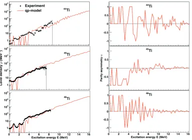
Fig. 4.Left panel: The nuclear level density (filled squares) of 46_{Ti. At low excitation energies, the data are} normalized (between the arrows) to known discrete levels (solid line). At higher excitation energies, the data are normalized to the BSFG level density (dashed line) going through the pointρ(Sn) (open square). For comparison

a data point obtained from Ericson fluctuations are shown (black triangle) [15]. Right panel: Experimentalγ-SF for46_{Ti (squares). For comparison, GEDR data from the (γ,abs) reaction are shown (triangles) [17].}

The normalizedγ-SF is shown in the right panel of Fig. 4. For comparison, the GEDR data [17] are also shown, which have been translated from photo neutron cross sectionσtoγ-SF by [16]

f(Eγ)= 1 3π2

~2c2 σ(Eγ)

Eγ . (5)

Unfortunately, there is a large energy gap between our data ending atEγ = 10 MeV and the GEDR data that start at 14 MeV.

4 Single-particle levels

The44,45,46Ti isotopes have 2 protons outside theZ =20 shell gap and 2, 3 or 4 neutrons outside the

N = 20 shell gap, respectively. The40_{Ca core is probably not very pronounced since these isotopes} have a nuclear quadrupole deformation of∼0.3. Experimentally, this is indicated by a level in45_Ti ofIπ=3/2+from theνd3/2single particle hole state appearing at low excitation energy.

The few active particles reveal very different level densities for the three isotopes, as shown in the left panel of Fig. 5. At around 8 MeV of excitation energy, the level densities show only∼500 MeV−1_. In the170,171,172Yb isotopes (left panel of Fig. 5) the number of levels is∼10.000 times larger. Here, the level densities for the even-even nuclei are almost identical, whereas the odd-mass nucleus has a factor 5−7 times more levels due to the unpaired valence neutron.

We have used a combinatorial quasi-particle model [7] to study the single-particle Nilsson orbitals involved in building the nuclear level density. The model also gives spin distributions as well as the parity distribution defined by the parity asymmetry parameter:

α=ρ+−ρ− ρ₊+ρ−

Fig. 5.Comparison between the level densities of44,45,46_{Ti and}170,171,172_{Yb. Typically, rare earth nuclei show} parallel level densities (in log scale) and the odd-mass nucleus reveals 5-7 times more levels than its even-even neighbors.

Excitation energy E (MeV)

0

2

4

6

8

10

)

-1

(MeV

ρ

Level density

1

10

2

10

3

10

4

10

x1

5.5-10.0 MeV

x3

8.5-10.0 MeV

x9

7.0-8.5 MeV x27

5.5-7.0 MeV

Fig. 7.Level density extracted from statistically independent data sets, taken from various initial excitation energy binsEi(the three upper curves). The lower curve is the result for the whole energy region of 5.5<Ei<10 MeV.

Figure 6 shows a nice reproduction of the observed level densities in the44,45,46Ti isotopes. At 8 MeV of excitation energy only about 6 proton and 6 neutron Nilsson orbitals are active. The cor-responding number for ytterbiums is more than 30 orbitals of each type. In the later case, there are enough levels with all spins and parities to reveal all types of transitions, and thus the universalγ-SF can be observed.

The level densities seem to increase most strongly around 3−4 MeV of excitation energy. Here, the first Cooper pair is probably broken, producing more states. Above 3−4 MeV, the parity asymmetry approaches zero on the average. However, below this excitation energy, the parities are predominately positive for the even titaniums, and negative for the odd case, which states the importance of the f7/2 orbitals at low excitation energies.

5 The

γ

-SF at various excitation regions

(MeV) γ E

0 2 4 6 8 10

-8 10

= 5.4-5.9 MeV

i

E

(MeV) γ E

0 2 4 6 8 10

-8 10

= 6.6-7.1 MeV

i

E

(MeV)

γ

E

0 2 4 6 8 10

)

-3

RSF (MeV

-8 10

= 7.8-8.3 MeV

i

E

(MeV) γ E

0 2 4 6 8 10

-8 10

= 9.0-9.4 MeV

i

E

(MeV)

γ

E

0 2 4 6 8 10

-8

10

Two last RSFs

(MeV) γ E

0 2 4 6 8 10

-8 10

= 6.0-6.5 MeV

i

E

(MeV) γ E

0 2 4 6 8 10

-8 10

= 7.2-7.7 MeV

i

E

(MeV) γ E

0 2 4 6 8 10

-8 10

= 8.4-8.9 MeV

i

E

(MeV) γ E

0 2 4 6 8 10

-8 10

= 9.6-10.0 MeV

i

E

(MeV)

γ

E

0 2 4 6 8 10

-8

10

All RSFs

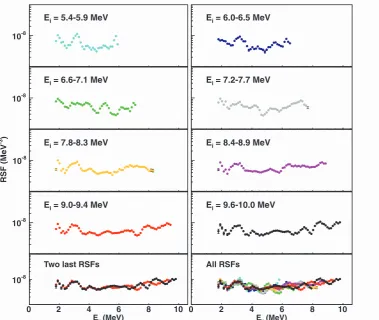
Fig. 8. Deduced γ-SF from various initial excitation bins Ei. The functions are evaluated from the ratio

P(Ei,Eγ)/ρ(Ef) as described in the text.

In order to study the variations in theγ-SF with excitation energy, we introduce here a new ap-proach [6]. By accepting one common level density, we may investigate the transmission coefficient in detail, and thus the validity of the Brink hypothesis.

We first adopt the solutionsT andρfrom Sec. 3 and rewrite expression (1) as

N(Ei)P(Ei,Eγ)≈ T(Eγ)ρ(Ei−Eγ). (7)

The normalization factor for each initial excitation bin is defined by

N(Ei)= REi

0 dEγT(Eγ)ρ(Ei−Eγ) REi

0 dEγP(Ei,Eγ)

. (8)

Since there exists only one common level density, we construct the counterpart to Eq. (7) in the case that the transmission coefficient depends on the initial excitation energy:

N0(Ei)P(Ei,Eγ)≈ T(Ei,Eγ)ρ(Ei−Eγ), (9)

whereN0 is determined analogously to Eq. (8). We expect thatT(Ei,Eγ) fluctuates on the average aroundT(Eγ). Thus, it is reasonable to expect thatN0_{≈ N, which gives a transmission coefficient of:}

T(Ei,Eγ)≈ N(Ei)

P(Ei,Eγ) ρ(Ei−Eγ)

or

T(Ef,Eγ)≈ N(Ef+Eγ)

P(Ef +Eγ,Eγ) ρ(Ef)

. (11)

In the last expression, the transmission coefficient is given as a function of final excitation energy

Ef =Ei−Eγ.

Roughly speaking, this treatment determines the transmission coefficient by dividing the first-generation matrix by the level density, i.e.T =P/ρ. This, allows in principle to determineT in small steps of initial or final excitation energies.

Figure 8 shows that the strength functions vary with initial excitation energy. Plotting allγ-SF together in the lower left panel, display a rather chaotic pattern where the functions deviate by of a factor 2−3. However, if we compare the two last functions, they look similar forγ-energies up to 7 MeV. Thus, it simply looks like levels below 3−4 MeV of excitation energy introduce the large fluctuations in theγ-strength.

The decay in quasi-continuum can be further investigated. In order to study theγ-SFs obtained from regions of higher level density, we have taken the four highest gates shown in Fig. 8 and only considered data withEγ<5.1 MeV. Thus, these statistically independentγ-SFs are evaluated in quasi-continuum with initial and final excitation energies of roughlyEi=8−10 MeV andEf =3−7 MeV, respectively. The deduced γ-SFs are presented in the upper panel of Fig. 9. In the lower panel the

(MeV) γ E

2 2.5 3 3.5 4 4.5 5

)

-3

MeV

-9

RSF (10

0 2 4 6 8 10 12 14 16

-9

10 ×

= 7.8-8.3 MeV

i

E

= 8.4-8.9 MeV

i

E

= 9.0-9.4 MeV

i

E

= 9.6-10.0 MeV

i

E

(a)

(MeV)

γ

E

2 2.5 3 3.5 4 4.5 5

Difference in RSF (%) -20

-10 0 10

20 (b)

relative deviations from the averageγ-SF are displayed. Here, we find typical∼6 % fluctuations that might be comparable with the Porter-Thomas fluctuations expected in the quasi-continuum of these light nuclei.

6 Summary

The level density andγ-strength function for titaniums have been determined using the Oslo method. Similar level density functions have been extracted from statistically independent data sets covering different excitation energies. This gives confidence to the Oslo method, since the disentanglement of the level density by Fermi’s golden rule predicts one and only one unique level density, independent of the data set.

The deducedγ-SF displays an enhancement at lowγ-ray energy where we see a bump around 3 MeV and another structure at energies near 2 MeV. A similar enhancement (upbend) has been seen in several other light-mass nuclei and is still not accounted for by present theories.

A method to study the evolution of theγ-SFs as a function of initial and final energy regions has been described. The deducedγ-SFs are found to display strong variations for different initial and final excitation energies if transitions to the lowest excitations are involved. The reason for the violent fluctuations of a factor of 2−3 is that only a few isolated levels are present at low excitation energies withEf <3 MeV. The differences in theγ-SFs obtained from a few number of transitions, that can be explained as a consequence of Porter-Thomas fluctuations of individual intensities, show that this energy region cannot be used for determination of the universalγ-SF.

However, the present work shows that it is possible to get more precise experimental information on the universalγ-SF. By imposing restrictions on the initial and final excitation energies, theγ-SFs for the decay between states in quasi-continuum can be extracted (i.e. forEf &3 MeV). The results from this selected data set show that the decay is consistent with aγ-SF which is independent of excitation energy within less than∼6 % already at these relatively low excitations. Thus, provided that we use data from the quasi-continuum, a universalγ-SF in the light mass region of the46_{Ti nucleus can be} extracted.

References

1. S.S. Dietrich and B.L. Berman, At. Data Nucl. Data Tables38, 199 (1988).

2. U. Agvaaluvsan, A. Schiller, J.A. Becker, L.A. Bernstein, P.E. Garrett, M. Guttormsen, G.E. Mitchell, J. Rekstad, S. Siem, A. Voinov, and W.Younes, Phys. Rev. C70, 054611 (2004). 3. S.G. Kadmenskii, V.P. Markushev, and V.I. Furman, Yad. Fiz.37, 227 (1983).

4. J. Bardeen, L.N. Cooper, and J.R. Schrieffer, Phys. Rev.108, 1175 (1957).

5. A.C. Larsen, M. Guttormsen, M. Krti˘cka, E. B˘et´ak, A. B¨urger, A. G¨orgen, H.T. Nyhus, J. Rekstad, A. Schiller, S. Siem, H.K. Toft, G.M. Tveten, A. Voinov and K. Wikan, Phys. Rev. C 83, 034315 (2011).

6. M. Guttormsen, A.C. Larsen, A. B¨urger, A. G¨orgen, S. Harissopulos, M. Kmiecik, T. Kon-stantinopoulos, M. Krti˘cka, A. Lagoyannis, T. L¨onnroth, K. Mazurek, M. Norrby, H.T. Nyhus, G. Perdikakis, A. Schiller, S. Siem, and A. Spyrou, N.U.H. Syed, H.K. Toft, G.M. Tveten, and A. Voinov, Phys. Rev. C83, 014312 (2011).

7. N.U.H. Syed, A.C. Larsen, A. B¨urger, M. Guttormsen, S. Harissopulos, M. Kmiecik, T. Kon-stantinopoulos, M. Krti˘cka, A. Lagoyannis, T. L¨onnroth, K. Mazurek, M. Norrby, H.T. Nyhus, G. Perdikakis, S. Siem, and A. Spyrou, Phys. Rev. C80, 044309 (2009).

8. A.C. Larsen, S. Goriely, A. B¨urger, M. Guttormsen, A. G¨orgen, S. Harissopulos, M. Kmiecik, T. Konstantinopoulos, M. Krti˘cka, A. Lagoyannis, T. L¨onnroth, K. Mazurek, M. Norrby, H. T. Ny-hus, G. Perdikakis, A. Schiller, S. Siem, and A. Spyrou, N.U.H. Syed, H.K. Toft, G.M. Tveten, and A. Voinov Phys. Rev. C, (2011), to be published.

10. A. Schiller, L. Bergholt, M. Guttormsen, E. Melby, J. Rekstad, and S. Siem, Nucl. Instrum. Meth-ods Phys. Res. A447, 498 (2000).

11. M. Guttormsen, T.S. Tveter, L. Bergholt, F. Ingebretsen, and J. Rekstad, Nucl. Instrum. Methods Phys. Res. A374, 371 (1996).

12. M. Guttormsen, T. Ramsøy, and J. Rekstad, Nucl. Instrum. Methods Phys. Res. A255, 518 (1987). 13. Data extracted using the NNDC On-Line Data Service from the ENSDF database.

14. D.M. Brink, Ph.D. thesis, Oxford University, 1955.

15. Merico Salas-Bacci, Steven M. Grimes, Thomas N. Massey, Yannis Parpottas, Raymond T. Wheller, and James E. Oldendick, Phys. Rev. C70, 024311 (2004).

16. RIPL-3 Handbook for calculation of nuclear reaction, (2009); available at http:// www-nds.iaea.org/RIPL-3/