Sharif University of Technology
Scientia IranicaTransactions E: Industrial Engineering www.scientiairanica.com
A multi-objective robust optimization model for
location-allocation decisions in two-stage supply chain
network and solving it with non-dominated sorting ant
colony optimization
J. Bagherinejad
and M. Dehghani
Department of Industrial Engineering, Faculty of Engineering and Technology, Alzahra University, Tehran, Iran. Received 29 October 2013; received in revised form 11 July 2014; accepted 28 September 2014
KEYWORDS Robust multi-objective optimization; Location-allocation; Multi-vehicle; Uncertainty; Non-dominated sorting ant colony optimization; NSGA-II.
Abstract.This study proposes a new, robust objective model for capacitated multi-vehicle allocation of customers to potential Distribution Centers (DCs) under uncertain environment. Uncertainty is dened by discrete scenarios on demands where occurrence probability of each scenario is known. The optimization objectives are to minimize transit time and total cost, including opening cost, assumed for opening potential DCs and shipping cost from DCs to the customers, where considering dierent types of vehicles leads to a more realistic model and causes more conict in these two objectives. A swarm intelligence-based algorithm named Non-dominated Sorting Ant Colony Optimization (NSACO) is used as the optimization tool. The proposed methodology is based on a new variant of Ant Colony Optimization (ACO) customized in multi-objective optimization problem of this research. For ensuring the authenticity of the proposed method, the computational results are compared with those obtained by NSGA-II. Results show the advantages and the eectiveness of the used method in reporting the optimal Pareto front of the proposed model. Moreover, the optimal solutions of the robust optimization model are insensitive to the disturbance of parameters under dierent scenarios, thus the risk of decision can be eectively reduced.
© 2015 Sharif University of Technology. All rights reserved.
1. Introduction
Supply Chain Management (SCM) is a set of ap-proaches utilized to eciently integrate the suppliers, manufacturers, warehouses, and stores, so that the merchandise is produced and distributed at the right quantities, to the right locations, and at the right time, in order to minimize system-wide costs while satisfying service level requirements [1]. The above denition reveals that there are many independent entities in a
*. Corresponding author. Tel.: +98 21 8804 4040-2178 E-mail addresses: [email protected] (J. Bagherinejad); minadehghani [email protected] (M. Dehghani)
supply chain, each of which tries to maximize its own inherent objective functions in business transactions. This is a complicated problem as too many factors are involved and need more than one objective to be satised, simultaneously. In traditional SCM, the focus of the designs of supply chain network is usually on single objective, minimum cost, or maximum prot. However, the design, planning, and scheduling projects usually involve trade-os among dierent incompatible goals such as fair prot distribution among all mem-bers, customer service levels, ll-rates, safe inventory levels, volume exibility, etc. Hence, real supply chains are to be optimized simultaneously considering more than one objective. Many of the problems that occur in
supply chain optimization are combinatorial in nature, and picking a set of optimal solutions in the case of multi-objective formulations requires an algorithm that can eciently search the entire objective space, using small amounts of computation time. Literature shows that evolutionary and swarm intelligence-based algorithms perform well in this respect and give good optimal results when applied to many combinatorial problems.
Ecient allocation of customers to Distribution Centers (DCs) always plays an important role in developing a awless and reliable supply chain. In this paper, two-stage supply chain network, including the distribution centers and the customers are consid-ered. There are customers with uncertain demands and potential places which are candidates to serve as distribution centers called potential DCs.
Each of the potential DCs can be shipped to any of the customers. This study proposes the utility of a new swarm intelligence-based algorithm called Non-dominated Sorting Ant Colony Optimization algorithm (NSACO) and the Non-dominated Sorting Genetic Algorithm (NSGA-II) for simultaneous robust opti-mization of two objectives, including minimizing the total transit time and total cost.
2. Prior related works
Since this research concentrates on location-allocation decisions, robust multi-objective optimization using ant colony optimization algorithm and NSGA-II, this section deals with prior works related to all these areas. Many researchers worked on basic facility loca-tion problem formulaloca-tions recognized as static and deterministic which take constant, known quantities as inputs and derive a single solution to be implemented at one point in time. These fundamental location problems are categorized into median problems [2], covering problems [3], center problems [3], etc. Later, focus was shifted to location-allocation problems which simultaneously locate facilities and dictate ows be-tween facilities and demands. Warszawski and Peer (1973) [4] are among the rst who studied the multi-commodity location problem. Their models consider xed location costs and linear transportation costs and assume that each warehouse can be assigned at most one commodity.
In literature, another set of problems is called xed charge facility location problems which consider xed charge associated with locating at each poten-tial facility site. There are two types of problems, including capacitated and uncapacitated plant loca-tion problems. Uncapacitated and capacitated plant location models are extensively dealt with in [5] and capacitated plant location models in [6]. Hajiaghaei-Keshteli (2011) [7] considered two stages of supply
chain network including Distribution Centers (DCs) and customers. His proposed model selects some potential places as distribution centers in order to supply demands of all customers; and in order to solve the given problem, two algorithms, genetic algorithm and articial immune algorithm, were developed.
Dierent methodologies are found in the literature for treating multi-objective optimization problems. These are the weighted-sum method, the "-constraint method, the goal-programming method, fuzzy method, etc. [8]. Zhou et al. (2003) [9] proposed a mathe-matical model and an ecient solution procedure for the bi-criteria allocation problem involving multiple warehouses with dierent capacities. The Bi-criteria Multiple Warehouse Allocation Problem (BMWAP) is similar to the well-known generalized assignment problem, but it is more challenging to solve due to its multiple criteria structure.
Ordonez and Zhao (2007) [10] investigated the robust capacity expansion problem of network ows under demand and travel time uncertainty. They provided complexity results for the two-stage network ow and design problem. Further, the problem of locating a competitive facility in the plane in the presence of uncertain demand was studied in [11] with a deviation robustness criterion. Baron et al. (2011) [12] applied robust optimization to the problem of locating facilities in a network facing uncertain demand over multiple periods. They considered a multi-period xed-charge network location problem for which they show that dierent models of uncertainty lead to very dierent solution network topologies, with the model with box uncertainty set opening fewer, larger facilities. Gabrel et al. (2011) [13] investigated a robust version of the location transportation problem with an uncertain demand using a two-stage formulation. The resulting robust formulation is a convex (nonlinear) program, and the authors apply a cutting plane algorithm to solve the problem exactly. Gulpinar et al. (2013) [14] considered a stochastic facility location problem in which multiple capacitated facilities serve customers with a single product, with uncertain customer de-mand and a constraint on the stock-out probability. Ghahtarani and Naja (2013) [15] proposed a robust optimization model for the multi-objective portfolio selection problem that uses a Goal Programming (GP) approach.
Non-dominated Sorting Genetic Algorithm II (NSGA-II), multi-objective ACO (MOACO), and Multi-Objective PSO (MOPSO) are few examples of multi-objective metaheuristic optimization algorithms of this type [16]. Chan and Kumar (2009) [17] dis-cussed a Multiple Ant Colony Optimization (MACO) approach in an eort to design a balanced and ecient supply chain network that maintains the best balance of transit time and customer service. The focus of their
paper is on the eective allocation of the customers to the DCs with the two-fold objective of minimization of the transit time and degree of imbalance of the DCs. Kalhor et al. (2011) [18] proposed a non-dominated archiving ant colony approach to solve the stochastic time-cost trade-o optimization problem. Mostafavi and Afshar (2011) [19] used a powerful ant colony algorithm known as non-dominated archiving multi-colony ant algorithm (NA-ACO) to solve the optimal Waste Load Allocation as a multi-objective optimization problem. Srinivas and Deb (1994) [20] used the non-dominated sorting concept on the GA. Then, NSGA-II, which was proposed by Deb et al. (2000) [21], is one of the most ecient and famous multi-objective evolutionary algorithms. Bhattacharya and Bandyopadhyay (2010) [22] solved the conicting bi-objective facility location problem with certain de-mand by NSGA II evolutionary algorithm. Shankar et al. (2013) [23] proposed a bi-objective optimization of supply chain design and distribution operations using Multi-Objective Hybrid Particle Swarm Opti-mization algorithm (MOHPSO). This heuristic incor-porates non-dominated sorting procedure to achieve bi-objective optimization of two conicting objectives. Sadeghi et al. (2014) [24] proposed a hybrid vendor managed inventory and redundancy allocation opti-mization problem in supply chain management, and they used NSGA-II for solving their problem.
The above literature review indicates that very little research has been carried out to implement swarm intelligence-based algorithms in robust multi-objective optimization for supply chain network. The purpose of this paper is to formulate and analyze a location-allocation model for a multi-vehicle single product in two-stage Supply Chain (SC) network with respect to the conicting objectives including minimizing total transit time and total cost, using NSACO and NSGA-II algorithms. The total cost involves opening cost assumed for opening potential DCs and shipping cost from DCs to the customers. The proposed model should lead to a nal two-stage SC design which would represent the desired compromise among the dierent objectives from the decision-maker's perspective.
3. Background
3.1. Multi-objective optimization
Multi-objective optimizations concerned with mathe-matical optimization problems involve more than one objective function to be optimized simultaneously. To obtain the optimal solution, there will be a set of optimal trade-os between the conicting objectives, where the set of optimal solution is known as Pareto front. A multi-objective optimization problem is dened as the maximization or the minimization of many objectives subject to equality and inequality
constraints. The multi-objective optimization problem can be formulated as follows:
Max:=Min:fi(x); i = 1; :::; Nobj: (1)
Subject to constraints: gj(x) = 0; j = 1; :::; M;
hk(x) 0; k = 1; :::; K; (2)
where fi is the ith objective function, x is the decision
vector, Nobj is the number of objectives, gj is the
jth equality constraint, and hk is the kth inequality
constraint.
There are techniques such as weighting methods and "-constraint method which transfer multi-objective problems to a single-objective one, using dierent com-binations of a weighting vector and constraints. Thus, each optimal solution can be assigned to a specic combination of weighting vector and constraint. Hence, in each run of the algorithm, a single solution can be achieved. However, multi-objective metaheuristic algorithms are capable of nding almost all candidate solutions (Pareto) in a single run. Metaheuristic algorithms can perform optimal/near-optimal solu-tions in all types of problems (linear/nonlinear, dis-crete/continuous, convex/non-convex) especially with incomplete or imperfect information or limited compu-tation capacity.
A set of solutions resulting from a program run, without using any techniques such as the weight-ing approach that are directly related to decision-makers' opinions, is the most important advantage of metaheuristic algorithms in the eld of multi-objective optimization. In this paper, two multi-objective metaheuristic algorithms, the NSGA-II and NSACO algorithm are used as optimization tools in extraction solution of the developed deterministic and non-deterministic models.
3.2. Robust multi-objective optimization
Many real-world optimization problems are subject to uncertainties and noise. These uncertainties and noise are caused by manufacturing errors, measurement errors, external factors, and inability to predict the future events. The uncertainties emerge in dierent parts of the optimization process.
One of the basic assumptions in stochastic pro-gramming is that the probability distribution function of the uncertain parameter is known. The goal of the stochastic model is often to obtain an optimal solution, which can minimize the expected value of the objective. However, in robust optimization, the uncertain parameters are described by the discrete scenarios or a continuous range. Robust optimization is an approach that deals with the uncertainty parameters
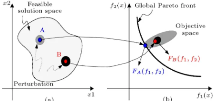
Figure 1. Eects of robust and sensitive solutions on objective functions.
in mathematical models and guarantees the feasibility of the solutions. The goal of this optimization method is to obtain an optimal solution, which is insensitive to almost all the samples of the uncertain parameters. Some minor deviations in the input variables of a system to be optimized may result in great deviations in the objective function values. The goal of robust optimization is not only to optimize the objectives, but also to take care of deviations of objective function val-ues caused by small or large changes or uctuations in the input variables. For multi-objective optimization, this means that, instead of looking for the global non-robust Pareto front, one is looking for the global non-robust Pareto front that means the Pareto fronts for dierent levels of uncertainty. Figure 1 illustrates the concept of the robustness of the solutions, where Figure 1(a) corresponds to the solution space (x1 and x2) and
Figure 1(b) represents the objective space (f1and f2).
For illustration purpose, it is assumed that we deal with minimization problem of two objective func-tions for which solufunc-tions A and B are found. As seen in Figure 1, solution A is better than solution B since both objective functions of solution A are smaller than those of solution B. However, let us assume that any uctuation occurs in the solutions as depicted by a circle in Figure 1(a). The uctuation of solution A is denoted by light gray circle and that for solution B is shaded by dark gray circle. Under these uctuated conditions, the corresponding objective functions also show some perturbations which are depicted by ellipses in Figure 1(b). It is noteworthy that solution A shows large dispersion in objective space, whereas solution B is just perturbed by a small amount in objective space. Considering the worst condition, solution B is preferred to solution A, because the maximally per-turbed objective functions of solution A are larger than those of solution B. Thus, solution A is inferior to the solution B in the worst case. In other words, solution B is more insensitive to the perturbation in terms of objective functions, and such insensitive solutions are said to be robust [25]. The robust optimization includes some formulations as regret model, variability model, and some other denitions such as the worst case
analysis, which includes two principles named minimax and maximin [26].
To achieve robustness in the solutions, the regret model is used in this research. In regret model, the regret value of the scenario is described by the dierence between the objective value of the feasible solution and the best objective value. It can be denoted by the absolute dierence or relative dierence. In the bi-objective problem, let S denote the set of scenarios. For 8s 2 S, x is the feasible solution of the deterministic programming model, Ps, while Z1s(x)
and Z2s(x) are the objective values of Ps with the
solution x; Z
1s and Z2s are the optimal objective
values of Ps. Given a constant !1, !2 > 0, if
[Z1s(x) Z1s ] =Z1s !1 and [Z2s(x) Z2s ] =Z2s !2
under every scenario s 2 S, then x is the robust solution of Ps. (Z1s(x) Z1s) and (Z2s(x) Z2s ) are
the absolute regret values and [Z1s(x) Z1s] =Z1s and
[Z2s(x) Z2s ] =Z2s are the relative regret values. !1
and !2 are the regret coecients. There might be
several robust solutions, and the best robust solution should be found out. Thus, the following model can be obtained:
Pro: min
X
s
sZ1s(x);
minX
s
sZ2s(x): (3)
Subject to:
[Z1s(x) Z1s ] =Z1s !1;
[Z2s(x) Z2s ] =Z2s !2: (4)
For 8s 2 S, s denotes the probability of scenario s,
where Pss=1s = 1. The optimal Pareto solutions of
the above model are the best robust solutions (robust Pareto front) of the original problem [26].
4. Description of problem and model
In this paper, a location-allocation model for multi-vehicle single product in two-stage supply chain net-work is developed. This model includes distribution centers, and customers with respect to two conicting objectives consist of minimizing total transit time and total cost. The total cost here involves opening cost, assumed for opening potential DCs, and shipping cost, from DCs to the customers. The proposed model selects some potential places as distribution centers in order to supply demands of all customers. It is assumed that distribution centers have unequal capacities, and each customer must be served from a single distribution center. Uncertainty is dened by discrete scenarios on demands where occurrence probability of each scenario
is known. Considering dierent types of vehicles lead to a more realistic model and cause more conict in the two objectives of the proposed problem, since a fast vehicle (because of high technology or having low capacity) has more cost, and a vehicle with low cost can lead to higher transit time.
According to Section 3.2, to solve the robust optimization model, we need the optimal objective values of the deterministic optimization model; we rst dene the multi-objective model with deterministic demand, and then, we formulate the robust multi-objective model with uncertain demand.
4.1. Multi-objective model with deterministic demand
Let us denote I as a set of nodes representing m customers, J as a set of nodes representing p potential distribution centers (locations), V as a set of types of vehicles for transferring process so that the number of vehicles is assumed to be unlimited, and E as a set of edges representing a connection between customers and DCs. di denotes the demand of customer i; fj
is the xed cost for opening a potential DC at site j; qv is the capacity of type of vehicle v, v 2 V ;
and the associated capacity qj for such DC; dij is the
distance between DC j and customer i; cv
ij is the cost
of assigning customer i to DC located at site j with type of vehicle v; and tv
ij is the transit time between
customer i to DC located at site j with type of vehicle v. All parameters introduced above are assumed to be non-negative. The binary variable yj is 1 if a DC
is located at site j and 0 otherwise. Similarly, binary variable xv
ij is equal to 1 if customer i is served by
the DC located at site j with type of vehicle v 2 V and 0 otherwise. The bi-objective capacitated multi-vehicle allocation of customers to distribution centers problem can be formulated as the following binary integer programming:
min z1= V X v=1 p X j=1 m X i=1
didijcvijxvij+ p
X
j=1
fjyj; (5)
min z2= V X v=1 p X j=1 m X i=1 tv
ijxvij: (6)
Subject to: V X v=1 p X j=1 xv
ij = 1; i = 1; :::; m; (7)
V X v=1 m X i=1
dixvij qjyj; j = 1; :::; p; (8)
m X i=1 p X j=1
dixvij qv; v = 1; :::; V; (9)
xv
ij; yj 2 f0; 1g; 8i = 1; :::; m; 8j = 1; :::; p;
8v = 1; :::; V: (10) The objective function (Eq. (5)) minimizes the total cost of opening distribution centers and assigning customers to such distribution centers, while objective function (Eq. (6)) minimizes total transit time between distribution centers and customers allocated to them. Constraints (Eq. (7)) guarantee that each customer is served by exactly one DC and also guarantee that each customer's demand is transferred by exactly one vehicle, while capacity constraints (Eq. (8)) ensure that the total demand assigned to a DC cannot exceed its capacity. The constraints (Eq. (9)) ensure that the total demand transferred by a vehicle cannot exceed its capacity. In this paper, capacity constraints of DCs have been relaxed through considering penalty function. In general, a penalty function approach is as follows. Given an optimization problem:
min f(X); s.t. X 2 A;
X 2 B; (11)
where X is a vector of decision variables, the con-straints \X 2 A" are relatively easy to satisfy, and the constraints \X 2 B" are relatively dicult to satisfy. The problem can be reformulated as:
min f(X) + p (d(X; B)) ;
s.t. X 2 A; (12)
where d(X; B) is a metric function describing the distance of the solution vector X from the region B, and p(0) is a monotonically non-decreasing penalty function such that p(0) = 0. Furthermore, any optimal solution of Eq. (12) will provide an upper bound on the optimum for Eq. (11), and this bound will be in general tighter than that obtained by simply optimizing f(X) over A.
In this paper, the objective functions are as follows:
min ^z1= z1+ 1:V i;
min ^z2= z2+ 2:V i; (13)
where 1:V i and :V i are penalty functions. 1 and
2 are two positive coecients where they are usually
considered greater than max(z1) and max(z2),
respec-tively. Also, V i represents relatively the violation of the value of capacity constraints related to DCs (Eq. (8)):
V i = XV
v=1 m
X
i=1
dixvij qjyj
! =qjyj;
if XV
v=1 m
X
i=1
dixvij> qjyj; j = 1; :::; p: (14)
And also:
V i = 0; if XV
v=1 m
X
i=1
dixvij qjyj; j = 1; :::; p:
Besides fullling other constraints (Eqs. (7) and (9)), the solutions with V i = 0 are feasible, otherwise the solutions are infeasible.
4.2. The robust multi-objective model with uncertain demand
As mentioned in Section 3.2, the formulation of the regret model is applied in this paper. It is assumed that the demand is uncertain in the future with several possible scenarios, while the other parameters are deterministic. The parameters in the robust model are all deterministic under a certain scenario s. Hence, in each scenario, the distribution center location and allocation problem can be described as a deterministic optimization model. In other words, for a non-deterministic model with S scenarios on demand, S deterministic models should be considered. For 8s 2 S, the optimal objective values of the deterministic optimization model is denoted by Z
1s and Z2s. x is
feasible under all scenarios, and Z1s(x) and Z2s(x)
denote the objective values of x under scenario s. Given the regret coecients (condence level), !1, and
!2 > 0, if and only if [z1s(x) z1s] =z1s !1 and
[z2s(x) z2s] =z2s !2 under every scenario s 2 S, x
is the robust solution of this problem. There might be several robust solutions, and the best robust solutions should be found out. Thus, the robust multi-objective optimization model (Pro) of capacitated multi-vehicle
location and allocation problem can be formulated as follows:
Pro: min z1= S
X
s=1
sz1s(x); (15)
min z2= S
X
s=1
sz2s(x): (16)
Subject to:
z1s(x) = V X v=1 p X j=1 m X i=1
disdijcvijxvij+ p
X
j=1
fjyj;
8s = 1; :::; S; (17)
z2s(x) = V X v=1 p X j=1 m X i=1 tv
ijxvij; 8s = 1; :::; S; (18)
V X v=1 p X j=1 xv
ij= 1; 8i = 1; :::; m; 8s = 1; :::; S; (19)
V X v=1 m X i=1
disxvij qjyj; 8j = 1; :::; p; 8s = 1; :::; S;
(20) m X i=1 p X j=1
disxvij qv; 8v = 1; :::; V; 8s = 1; :::; S;
(21) [z1s(x) z1s] =z1s !1; (22)
[z2s(x) z2s] =z2s !2; (23)
xv
ij; yj2 f0; 1g; 8i = 1; :::; m; 8j = 1; :::; p;
8v = 1; :::; V: (24) In the above model, Eq. (15) is the rst objective, which is aiming at the total average cost in all sce-narios, while the second objective function Eq. (16) is aiming at the total average transit time in all scenarios. Eq. (22) and Eq. (23) ensure that the feasible solution of model Pro should meet the
re-quirement of the robust solution. The optimal Pareto solutions of the above model are the best robust solutions (robust Pareto front) of the original prob-lem.
5. Solution procedure
A main branch in the theory of computation, named computational complexity, considers classifying com-putational problems regarding their inherent diculty. Some important complexity classes are P, NP, NP-complete, NP-hard, EXP-space, EXP-time, P-space, etc. Many real-world optimization problems belong to the class of NP-hard, and in order to solve NP-hard problems, there are no provably ecient algorithms, i.e. exact methods cannot solve the problems in normal time. According to the performed studies, metaheuristic algorithms are suitable tools to optimize this class of problems [27]. Mirchandani and Francis (1990) [28] showed that Capacitated Facility Location Problem (CFLP) is NP-hard. Minoux (2010) [29] proved that the robust network design problem with uncertain demand is NP-hard. Since the proposed bi-objective models known in Sections 4.1 and 4.2 consist of the above NP-hard problems, these are NP-hard as well. This justies the use of a meta-heuristic algorithm. In this section, the well-known Multi-Objective Evolutionary Algorithm (MOEA) of NSGA-II and a new swarm intelligence based al-gorithm called Non-dominated Sorting Ant Colony Optimization (NSACO) are presented to solve the problem.
5.1. Non-dominated Sorting Genetic Algorithm-II (NSGA-II)
A population-based search MOEA can present a set of Pareto optimal solutions of multi-objective opti-mization problems involving two or more conicting objectives. One of these MOEAs that is frequently used in many optimization problems as the best technique to generate Pareto frontiers is the Non-dominated Sorting Genetic Algorithm-II (NSGA-II) proposed by Deb et al. (2000) [21]. To start NSGA-II, one rst randomly generates a population P1with size nP op chromosomes
(solutions) and then sorts the chromosomes in P1
into several fronts of non-dominated solutions. All chromosomes in this population are sorted into dif-ferent front levels based on the domination of pair comparison. Each front level is assigned a tness (or a rank) which equals its non-domination level. Level 1 is the top level in which the individual is dominated by none of the other chromosomes; level 2 is the secondary level in which the chromosome is dominated by some chromosomes only in level 1, and so on. Considering the obtained chromosomes using the tournament selection operator for P1, the ospring
population O1 is created with respect to the crossover
probability (Pc) and the mutation probability (Pm).
Moreover, the algorithm obtains the objective values of each chromosome in P1and O1.
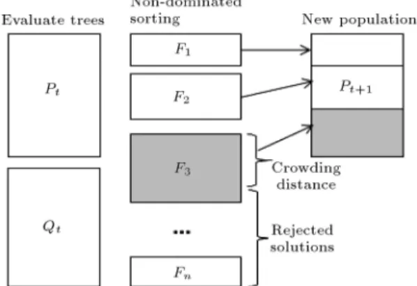
After merging P1 and O1 to form Rt, the
al-gorithm sorts Rt in several non-dominated fronts Fi,
where the best Fis form the next population Pt+1.
Since the size of Pt+1 is equal to the size of Pt,
all of the elements from a front cannot be in Pt+1.
Hence, when a front is added to Pt+1incompletely, the
crowding distance approach is applied. The crowding distance is an important concept proposed by Deb et al. (2000) [21] in his algorithm NSGA-II. It serves for getting an estimate of the density of solutions surrounding a particular solution in the population. Figure 2 shows the calculation of the crowding distance of point i which is an estimate of the size of the largest cuboid enclosing I without including any other points.
Figure 2. Crowding distance computation.
Figure 3. Graphical representation of NSGA-II.
In fact, the crowding distance is a measure of how close an individual is to its neighbors. Consequently, the required population is organized from the top elements of the front without losing good solutions (elitism). The algorithm creates Ot+1from Pt+1using a crowding
distance method and crossover and mutation operators. Regarding the stopping criteria and iterating the above stages, the algorithm hopefully presents the best Pareto optimal solutions. Figure 3 shows a graphical representation of NSGA-II. For more details on the implementation of NSGA-II see [21,30].
5.2. Non-dominated sorting ant colony optimization method
Ant Colony Optimization (ACO) algorithms are the most successful and widely recognized algorithmic tech-niques based on real ant behaviors [31]. Several papers were proposed to extend the Ant Colony Optimization (ACO) method in order to handle a multi-objective optimization problem [17-19].
In this paper, a swarm intelligence-based al-gorithm named Non-dominated Sorting Ant Colony Optimization (NSACO) is proposed to tackle the bi-objective capacitated multi-vehicle allocation of cus-tomers to distribution centers problem in uncertain environment. NSACO algorithm is based on the same non-dominated sorting concept used in NSGA-II. The proposed methodology is based on a new variant of ACO specialized in multi-objective optimization problem. Steps of the NSACO are as follows.
In the rst step, a colony of ants with size nAnt is considered. Then, ACO parameters such as , , , etc. are initialized, where and are parameters used for controlling the exponential weight of the pheromone trail and the heuristic exponential weight, respectively, and is evaporation rate [31]. Also in this step, the value of the initial pheromone trail, 0, is determined
and the tabu lists of all ants are constructed, which contain all the unvisited nodes for each ant and the list of optimal paths traversed by the ants. The initial pheromone intensity, ij, or the path from nodes i to j
In the second step, for each ant of the colony, a new solution using ACO probabilistic rule is created. It means that, for each ant, a DC vector, an allocation matrix and a vehicle vector are assigned. The DC vec-tor is a binary vecvec-tor that indicates the opening or not opening DCs, the allocation matrix is a binary matrix that indicates the allocation of customers to the located DCs, and the vehicle vector is an integer vector that indicates the type of vehicle for transferring customer's demand. The allocation matrix and vehicle vector form a three-dimensional decision variable named xv
ij. Then,
objective values for this solution are calculated and evaluated.
In order to construct the solution, ant k currently at node i determines the next node to visit, node j, by applying the sampling approach known as the Roulette Wheel Selection. For this purpose, rst, movement probability for ant k from node i to other nodes including the neighbors of the node i, must be calculated. Sk(i) is a Tabu list to avoid creating a loop,
containing those unvisited nodes for ant k currently at node i. Therefore, node j 2 Sk(i) is the node
randomly chosen from the list Sk(i) according to the
pseudo random proportional distribution rule Eq. (25) and the Roulette wheel selection [31]:
Pk
ij= ijij=
X
u2Sk(i)
iuiu
;
if j 2 Sk(i); otherwise Pijk = 0; (25)
where Pk
ij is the probability that ant k chooses to move
from node i to node j, and ijis a heuristic value which
equals to the inverse of the length from node i to node j, ijis the amount of pheromone trail of the path from
node i to node j, and are two parameters used for controlling the exponential weight of the pheromone trail and the heuristic value. Then, after calculating the probability values, the Roulette wheel selection is used to select next node among these existing neighbor nodes [32]. In this paper, this process is occurred three times for constructing the DC vector, the allocation matrix, and the vehicle vector.
In the third step, after all the ants of the colony traversed their paths, the non-dominated sort-ing method is applied, where the entire population is sorted into various non-domination fronts. In a minimization problem, a vector x(1) is partially less
than another vector x(2), x(1)< x(2)when no value
of x(2) is less than x(1) and at least one value of x(2)
is strictly greater than x(1) [33]. A solution which
is not partially less is a dominated solution and a solution which cannot be dominated throughout an existing solution set is called a non-dominated solution or Pareto front. The rst front being completely a non-dominant set in the current population and the second
front being dominated by the individuals in the rst front only and the front goes so on. Each individual in each front is assigned tness values or based on front in which they belong to. Individuals in the rst front are given a tness value of 1 and individuals in the second are assigned a tness value of 2 and so on. A major dierence of NSACO and NSGA-II is that in NSACO, an additional population because of operators like crossover and mutation is not generated, and population size always equals nAnt. Also, all ants of a colony are sorted based on quality and discipline factors, simultaneously. Therefore, in addition to the tness value, a parameter called crowding distance is calculated for each ant to ensure the best distribution of the non-dominated solutions.
Once the non-dominated solutions are found, other (dominated) solutions are discarded and once again the pheromone trails are updated and evapora-tion process is occurred according to non-dominated solutions. In this paper, three pheromone trails matrix are designed for DC vector, allocation matrix and vehicle vector. The pheromone trails matrix for DC vector is a 2 p dimensions matrix, in which 2 is identied as open or closed state of each DC, that the rst row and the second row are considered for closing and opening the DCs, respectively, and p is identied as the number of DCs (Eq. (26)). The pheromone trails matrix for allocation matrix is a pm dimensions matrix, in which p and m are identied as number of DCs and number of customers, respectively (Eq. (27)), and the pheromone trails matrix for vehicle vector is a V m dimensions matrix, in which V and m are identied as types of vehicles and number of customers, respectively (Eq. (28)).
1 =
11 : : 1p
21 : : 2p
; (26)
2 =
11 : : 1m
p1 : : pm
; (27)
3 =
11 : : 1m
v1 : : vm
: (28)
The heuristic information matrix for DC vector is a 2 p dimensions matrix, in which 2 is identied as closed or open state of each DC, in which the rst row and the second row are considered for xed cost for opening potential DCs and inverse of xed cost for opening potential DCs, respectively, and p is identied as the number of DCs (Eq. (29)). The heuristic information matrix for allocation matrix is a P m dimensions matrix, in which p and m are identied as number of DCs and number of customers, respectively, which contains inverse of distance values between customers and DCs (Eq. (30)), and the heuristic information
matrix for vehicle vector is a V m dimensions matrix, in which V and m are identied as types of vehicles and number of customers, respectively, which contains inverse of shipping cost from DCs to customers. There are three heuristic information matrices 8j = 1; :::; p (Eq. (31)).
1 =
f1 :: fp
1=f1 :: 1=fp
; (29)
2 = 2
41=d:11 :: 1=d:: :1m 1=dp1 :: 1=dpm
3
5 ; (30)
3 = 2
41=c:1j1 :: 1=c:: :mj1 1=c1jv :: 1=cmjv
3
5 : (31)
The pheromone trails are updated according to the non-dominated solutions in the Pareto front, and in order to prevent unlimited accumulation of the pheromone trails and help the algorithm to forget bad decisions of formers, evaporation process is applied on pheromone trails. This updating process aects the selection of new solutions using ACO probabilistic rule in the next iteration. This cycle is repeated for a pre-dened number of iterations known as Cycle Iteration. At the end of running this algorithm, the present non-dominated solutions in the last iteration are the opti-mal solutions of the multi-objective problem. Figure 4 shows a graphical representation of NSACO.
Figure 4. Graphical representation of NSACO.
5.3. Adaptive algorithms for solving the multi-objective robust optimization
In this paper, two metaheuristic algorithms, NSGA-II and NSACO, are proposed as the optimization tools. The algorithms are coded in MATLAB software and tested on a Core 2 Duo/2.66 GHz processor. Steps of adaptive algorithms for solving the multi-objective robust optimization model by NSGA-II and NSACO are as follows:
Step 1. Considering a for loop over the number of scenarios for demand;
Step 2. Solving the bi-objective deterministic model in all scenarios by NSGA-II or NSACO and saving the objective values of Pareto front, Z
1s
and Z
2s, in memory of algorithms;
Step 3. After optimizing the deterministic models in all scenarios, the rst three fronts of solutions for each model (each scenario) are considered together in a set named good solutions;
Step 4. For each solution in the set good solutions, feasibility survey is done according to the constraints (Eqs. (19), (20) and (21));
Step 5. The solutions that are feasible in all scenarios of demands simultaneously are stored in an archive named feasible solutions;
Step 6. For each solution in feasible solutions archive:
Step 6.1. Calculating objective values for each scenario (z1s(x) and z2s(x))
according to Eqs. (17) and (18);
Step 6.2. Feasibility survey according to the regret constraints (Eqs. (22) and (23));
Step 6.3. If all regret constraints are satis-ed for a solution, that solution is stored in an archive named robust solutions, as a robust solution.
Step 7. After nding all robust solutions and saving them to robust solutions archive, the objective values of each robust solution are calculated according to Eqs. (15) and (16);
Step 8. Non-dominated sorting and crowding distance methods are done on robust solutions archive;
Step 9. The robust Pareto front is found.
In this paper, sixteen numerical examples, in-cluding eight cases in small scale and eight cases in large scale are considered for experimental study which presents dierent levels of diculty for alternative solution approaches.
Initial population size is assumed 100 and 200 for small and large scales, respectively. Problem size diers from each other by changing DCs/customer's numbers, types of vehicles, and number of scenarios of demand.
6. Parameter tuning
In order to obtain solutions with better quality, the parameters of both algorithms are adjusted in this section using an auto tuning approach. For NSGA-II parameters, rst, some random numbers, for example, 10 numbers in the range 0.55 to 0.85, are selected randomly for Pc. This range is considered according
to existing literature in the eld of genetic algorithms. It could be considered in 0 to 1 in the most pessimistic case. For each random number in the range, NSGA-II algorithm runs, and the results are saved. Then, by observing the best solutions, we tried the next random numbers that could be close to the Pc of
the best solutions. In fact, after observing the best solutions, lower and upper bound of the range are updated according to good values of Pc. Exactly the
same procedure in the range 0 to 0.45 is repeated for Pm. This process is performed by an external NSGA-II
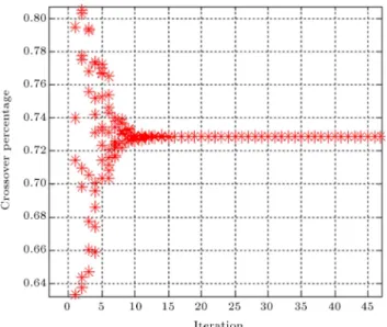
program for auto tuning parameters. Figures 5 and 6 show that Pc equals 0.73, and Pmequals 0.37.
As shown in these gures, Pc and Pm are tuned
in 15th iteration, approximately. If in each iteration, 10 random numbers are considered, Pc and Pm are
tuned with considering 150 times running of NSGA-II algorithm. As previously mentioned, for NSACO
Figure 5. Auto tuning parameters (crossover probability).
Figure 6. Auto tuning parameters (mutation probability).
parameters, some numbers, for example, 10 numbers in the range 0.8 to 1.8, are selected randomly for 1,
pheromone exponential weight for DC vector, and then by observing the best solutions, we tried the next random numbers that could be close to the 1 of the
best solutions.
Exactly the same procedure in the range 0.05 to 0.6 is repeated for 1, heuristic exponential weight
for DC vector. These initial ranges are considered according to both existing literature in the eld of ACO algorithm and some tentative running of NSACO program. This procedure is repeated for other parame-ters. This process is performed by an external NSACO program for auto tuning parameters.
The parameters of NSACO for all optimization cases are summarized in Table 1.
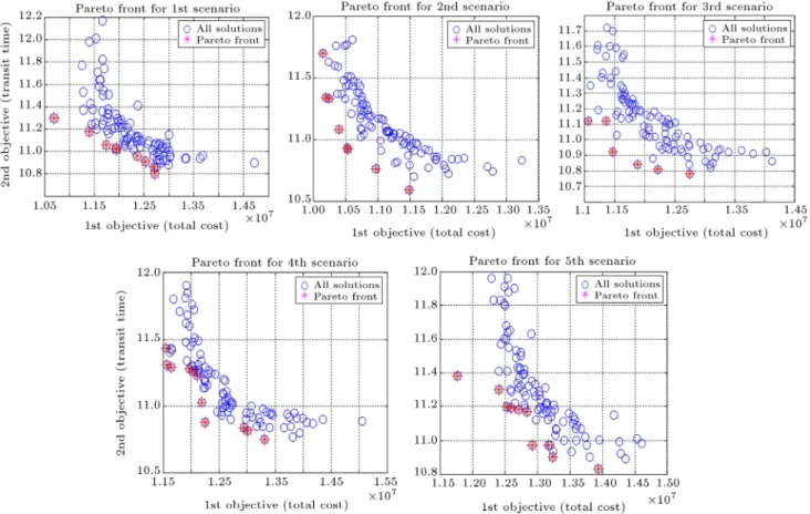
7. Performance evaluation of the algorithms To illustrate the performance of the used procedures to optimize the proposed models, problem 1 in small scale is considered as an example. As mentioned before, for solving the bi-objective robust model, rst, the deterministic models 8s 2 S should be solved. Figures 7 and 8 show the performance of the proposed
Table 1. NSACO parameters.
1 (Pheromone exponential weight for DC vector) 1.30
1 (Heuristic exponential weight for DC vector) 0.40
2 (Pheromone exponential weight for allocation matrix) 1.58
2 (Heuristic exponential weight for allocation matrix) 0.33
3 (Pheromone exponential weight for vehicle vector) 1.34
3 (Heuristic exponential weight for vehicle vector) 0.52
Figure 7. Pareto front of problem 1 in small scale by NSACO (3rd iteration with nAnt = 100).
Figure 9. Robust Pareto solutions by NSACO &
NSGA-II (problem 2 in small scale, in 200th iteration with npop = 100).
algorithm, NSACO, in the 3rd and 200th iterations with ve scenarios on demand.
Figure 9 shows all robust solutions and robust Pareto solutions for problem 2 in small scale as an example. Also, to view the output of the decision variables, the robust Pareto solutions of problem 6 in small scale are given in the Appendix.
To check the quality of solutions obtained by the NSACO, four evaluation metrics including: (1) Num-ber of Pareto solutions (NOS), (2) Maximum spread or diversity metric [34], (3) Mean Ideal Distance (MID) metric [35], and (4) time of running have been used. Diversity and MID metrics are formulated as follows:
Diversity = v u u tXm
j=1
max
n f j
n minn fnj
2
; (32)
MID =Xn
i=1
Ci
n; (33)
Figure 10. MID metric comparisons for problem 2 in small scale.
where in Eq. (32), m is the number of objectives, n is the number of Pareto solutions, and in Eq. (33), n is the number of Pareto solutions and Ci is the
distance of ith Pareto solution from ideal point ((0,0) in bi-objective minimization).
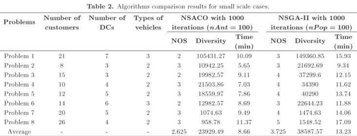
Figure 10 shows MID metrics comparison for problem 2 in small scale for rst scenario (determin-istic optimization). For better display, MID axis is considered under logarithmic scale. As shown in Figure 10, in the rst iterations, there are more infeasible solutions and they cause adding large penalty functions to objective values, but during the process of algorithm, the infeasible solutions, because of great objective values are discarded and objective values are more real and then convergence process goes smoothly. Tables 2 and 3 show the algorithms comparison re-sults for some small and large scale bi-objective robust optimization problems with iteration number 1000. From these results, it can be seen that the NSACO is more ecient than NSGA-II in the viewpoint of optimality, but, according to the Diversity and NOS,
Table 2. Algorithms comparison results for small scale cases. Problems Number of
customers
Number of DCs
Types of vehicles
NSACO with 1000 iterations (nAnt = 100)
NSGA-II with 1000 iterations (nP op = 100) NOS Diversity Time
(min) NOS Diversity
Time (min)
Problem 1 21 7 3 2 105431.27 10.09 3 149360.85 15.93
Problem 2 8 3 2 3 10942.25 5.65 3 21692.69 9.34
Problem 3 15 3 2 2 19982.57 9.11 4 37299.6 12.15
Problem 4 10 4 2 3 21503.86 7.03 4 34390 11.62
Problem 5 12 5 2 3 18559.97 7.86 4 40290 13.74
Problem 6 14 6 3 2 12982.57 8.69 3 22644.23 11.88
Problem 7 20 5 2 3 1074.63 9.49 4 1474.63 14.06
Problem 8 26 4 2 3 958.78 11.37 5 1548.52 17.09
Table 3. Algorithms comparison results for large scale cases. Problems Number of
customers
Number of DCs
Types of vehicles
NSACO with 1000 iterations (nAnt = 200)
NSGA-II with 1000 iterations (nP op = 200) NOS Diversity Time
(min) NOS Diversity
Time (min)
Problem 1 32 7 3 3 33058.6 34.77 4 52176 47.96
Problem 2 40 11 3 2 24265.1 43.25 4 46206 68.26
Problem 3 24 6 3 2 34265.05 27.86 5 43890.5 38.32
Problem 4 70 9 3 3 26744.7 65.13 4 38730 71.4
Problem 5 62 9 3 2 10300 57.56 3 37996 68.23
Problem 6 80 7 3 3 115782.5 70. 3 5 223900 88.2
Problem 7 68 11 3 2 10256 61.68 3 18957 76.9
Problem 8 60 10 3 3 11541 55.23 4 13628 73.2
Average - - - 2.5 33276.62 51.97 4 59435.44 66.56
Table 4. Statistical comparison results ( = 5%). Mann-Whitney test
Small scale cases Large scale cases P -value results P -value results NOS 0.005
NSGA-II is preferred to NSACO
0.002
NSGA-II is preferred to NSACO
Diversity 0.115
There were no signicant
dierences
0.074
There were no signicant
dierences
MID 0.048
NSACO is preferred to
NSGA-II
0.041
NSACO is preferred to
NSGA-II
Time 0.002
NSACO is preferred to
NSGA-II
0.046
NSACO is preferred to
NSGA-II
the NSGA-II has better distribution of solutions in the trade-o surface.
In this paper, in order to evaluate the performance of the two algorithms, the Mann-Whitney test is done by Statistical Package for the Social Sciences (SPSS 16.0) software (Table 4).
The regret coecients (condence level), !1 and
!2, are assumed the same (!, in this paper), where it
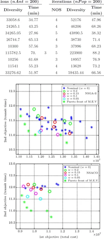
takes values between 0 and 100%. Figure 11 depicts the robust objective results for capacitated multi-vehicle allocation of customers to DCs problem with considering four values for !, including 5%, 10%, 15%, and 20%. When looking at the robust results, it is clear that the Pareto front shifts to higher values for both objectives when ! increases. The nominal case is related to the Pareto solutions of deterministic models in all scenarios.
Figure 11. Bi-objective location allocation: Pareto set by NSGA-II & NSACO (problem 1 in small scale in 500th iteration with npop = 100).
It has to be mentioned that the robust opti-mization model can obtain more insensitive solutions than the stochastic optimization like mean expected value model (M.E.V model, with considering mean ex-pected values of demand and solving with deterministic
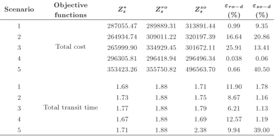
Table 5. Comparison between the results of stochastic optimization model and robust optimization model for problem 5 in small scale.
Scenario Objective
functions Zs Zsro Zsso
"ro d
(%)
"so d
(%) 1
Total cost
287055.47 289889.31 313891.44 0.99 9.35
2 264934.74 309011.22 320197.39 16.64 20.86
3 265999.90 334929.45 301672.11 25.91 13.41
4 296305.81 296418.94 296496.34 0.038 0.06
5 353423.26 355750.82 496563.70 0.66 40.50
1
Total transit time
1.68 1.88 1.71 11.90 1.78
2 1.73 1.88 1.75 8.67 1.16
3 1.77 1.88 1.79 6.21 1.13
4 1.67 1.88 1.69 12.57 1.19
5 1.71 1.88 2.38 9.94 39.00
model), especially when the data distribution is large compared to the average. The robust optimization model in the both objectives does not change a lot under all scenarios, thus the risk of decision can be eectively reduced.
Table 5 shows the comparison between the results of stochastic optimization model (M.E.V model) and robust optimization model. As an example, the rst member of Pareto front in each scenario for problem 5 in small scale is considered. The relative dierence between Zso
s and Zscan be obtained by:
"so d= f(Zsso Zs)=Zsg 100%:
The relative dierence between Zro
s and Zs can be
obtained by:
"ro d= f(Zsro Zs)=Zsg 100%;
where Z
s, Zssoand Zsroare the objective values of
deter-ministic model, stochastic optimization model (M.E.V model), and robust optimization model, respectively.
It can be concluded from Table 5 that the "so d
for 1st objective and 2nd objective is uctuating from 0.06 to 40.5% and 1.13 to 39%, respectively, while "ro d
for 1st objective and 2nd objective is uctuating from 0.038 to 25.91% and 6.21 to 12.57%, respectively. The latter is more stable.
8. Discussion and conclusion
Nowadays, the competition is vital for the rms' survival in SCs. Then, the basic priority for supply chain management should be designing the SC network properly, to gain competitive advantage. In this paper, a multi-objective robust optimization model for ca-pacitated multi-vehicle allocation of customers to DCs in two-stage SC considering distribution centers and customers is proposed. The optimization objectives are
to minimize transit time and total cost. Results show the trade-o between total transit time and total cost, since the dierent types of vehicles used in the model cause more conict in these two objectives.
In this paper, swarm intelligence-based algorithm named Non-dominated Sorting Ant Colony Optimiza-tion (NSACO) is presented to nd Pareto fronts. The proposed methodology is based on a new variant of Ant Colony Optimization (ACO) customized in multi-objective optimization problem. The crowding distance technique is used to ensure the best distribution of the non-dominated solutions.
For ensuring the robustness of the proposed method and giving a practical sense of this study, the computational results are compared with those obtained by Non-dominated Sorting Genetic Algo-rithms (NSGA-II). Results show the advantages and eectiveness of the used procedures in reporting the optimal Pareto front of the proposed deterministic and non-deterministic models.
Moreover, it can be seen that the NSACO is more ecient than NSGA-II in the viewpoint of optimality and running time saving, but the NSGA-II has bet-ter distribution of solutions in the trade-o surface. Also, the optimal solutions of the robust optimization model are insensitive to the disturbance of parameters under dierent scenarios, and the robust optimization model can obtain better solutions than the stochastic optimization model, thus the risk of decision can be eectively reduced.
Future research may develop the NSACO to increase the diversity of solutions. Additionally, it may be combined routing with location-allocation problem. Furthermore, given the successful application of a NSACO to the bi-objective warehouse allocation prob-lem, the used algorithm can be modied to obtain non-dominated solutions for warehouse allocation problems with more than two objectives.
References
1. Simchi-Levi, D. Kaminsky, P. and Simchi-Levi, E., Designing and Managing the Supply Chain, New York: Irwin McGraw-Hill (2000).
2. ReVelle, C. \The maximum capture or `sphere of inuence' location problem: Hoteling revisited on a network", Journal of Regional Science, 26(2), pp. 343-358 (1986).
3. Daskin, M.S., Network and Discrete Location: Models Algorithms and Applications, New York: Wiley (1995).
4. Warszawski, A. and Peer, S. \Optimizing the location of facilities on a building site", Operational Research Quarterly, 24, pp. 35-44 (1973).
5. ReVelle, C.S., Eiselt, H.A. and Daskin, M.S. \A bibliography for some fundamental problem categories in discrete location science", European Journal of Operational Research, 184, pp. 817-848 (2008).
6. Sridharan, R. \The capacitated plant location prob-lem", European Journal of Operational Research, 87, pp. 203-213 (1995).
7. Hajiaghaei-Keshteli, M. \The allocation of customers to potential distribution centers in supply chain net-works: GA and AIA approaches", Applied Soft Com-puting, 11, pp. 2069-2078 (2011).
8. Chen, C.L. and Lee, W.C. \Multi-objective optimiza-tion of multi-echelon supply chain networks, with uncertain product demands and prices", Computers and Chemical Engineering, 28, pp. 1131-1144 (2004).
9. Zhou, G., Min, H. and Gen, M. \A genetic algorithm approach to the bi-criteria allocation of customers to warehouses", International Journal of Production Economics, 86, pp. 35-45 (2003).
10. Ordonez, F. and Zhao, J. \Robust capacity expansion of network ows", Networks, 50, pp. 136-145 (2007).
11. Blanquero, R., Carrizosa, E. and Hendrix, E.M.T. \Locating a competitive facility in the plane with a robustness criterion", European Journal of Operational Research, 215, pp. 21-24 (2011).
12. Baron, O., Milner, J. and Naseraldin, H. \Facility location: A robust optimization approach", Production and Operations Management, 20, pp. 772-785 (2011).
13. Gabrel, V., Lacroix, M., Murat, C. and Remli \Ro-bust location transportation problems under uncertain demands", Combinatorial Optimization, Discrete Ap-plied Mathematics, 164(1), pp. 100-111 (2014).
14. Gulpinar, N., Pachamanova, D. and Canakoglu, E. \Robust strategies for facility location under uncer-tainty", European Journal of Operational Research, 225, pp. 21-35 (2013).
15. Ghahtarani, A. and Naja, A.A. \Robust goal pro-gramming for multi-objective portfolio selection prob-lem", Economic Modeling, 33, pp. 588-592 (2013).
16. Xing, H. and Qu, R. \A non-dominated sorting genetic algorithm for bi objective network coding based
mul-ticast routing problems", Information Sciences., 233, pp. 36-53 (2013).
17. Chan, F.T.S. and Kumar, N. \Eective allocation of customers to distribution centers: A multiple ant colony optimization approach", Robotics and Computer-Integrated Manufacturing, 25(1), pp. 1-12 (2009).
18. Kalhor, E., Khanzadi, M., Eshtehardian, E. and Afshar, A. \Stochastic time-cost optimization using non-dominated archiving ant colony approach", Au-tomation in Construction, 20, pp. 1193-1203 (2011).
19. Mostafavi, S.A. and Afshar, A. \Waste load alloca-tion using non-dominated archiving multi-colony ant algorithm", Procedia Computer Science, 3, pp. 64-69 (2011).
20. Srinivas, N. and Deb, K. \Multi-objective optimiza-tion using non-dominated sorting genetic algorithms", Evolutionary Computation, 2(3), pp. 221-248 (1994).
21. Deb, K., Agrawal, S., Pratap, A. and Meyarivan, T. \A fast elitist non-dominated sorting genetic algorithm for multi-objective optimization: NSGA-II", in Proceed-ings of the 6th International Conference on Parallel Problem Solving from Nature, pp. 849-58 (2000).
22. Bhattacharya, R. and Bandyopadhyay, S. \Solving conicting bi-objective facility location problem by NSGA II evolutionary algorithm", The International Journal of Advanced Manufacturing Technology, 51, Issue 1-4, pp. 397-414 (2010).
23. Shankar, B.L., Basavarajappa, S., Chen, J.C.H. and Kadadevaramath, R.S. \Location and allocation deci-sions for echelon supply chain network -A multi-objective evolutionary approach", Expert Systems with Applications, 40, pp. 551-562 (2013).
24. Sadeghi, J., Sadeghi, S. and Akhavan Niaki, S.T. \A hybrid vendor managed inventory and redundancy allocation optimization problem in supply chain man-agement: An NSGA-II with tuned parameters", Com-puters & Operations Research, 41, pp. 53-64 (2014).
25. Ok, S.Y., Lee, S.Y. and Park, W. \Robust multi-objective maintenance planning of deteriorating bridges against uncertainty in performance model", Advances in Engineering Software, 65, pp. 32-42 (2013).
26. Baohua, W. and Shiwei, H. \Robust optimization model and algorithm for logistics center location and allocation under uncertain environment", Journal of Transportation Systems Engineering and Information Technology, 9(2), Online English edition of the Chinese language journal (2009).
27. Talbi, E.G., Meta-Heuristics: From Design to Imple-mentation, New York: Wiley (2009).
28. Mirchandani, P.B. and Francis, R.L., Discrete Location Theory, New York: Wiley (1990).
29. Minoux, M. \Robust network optimization under-polyhedral demand uncertainty is NP-hard", Discrete Applied Mathematics, 158, pp. 597-603 (2010).
30. Deb, K., Multi-Objective Optimization Using Evolu-tionary Algorithms, England: John Wiley and Sons, Ltd (2001).
31. Dorigo, M. and Stutzle, T., Ant Colony Optimization, Cambridge, MA: MIT Press (2004).
32. Xia, X. \Particle swarm optimization method based on chaotic local search and roulette wheel mecha-nism", International Conference on Applied Physics and Industrial Engineering, Physics Procedia, 24(A), pp. 269-275 (2012).
33. Tamura, K. and Miura, S. \Necessary and sucient conditions for local and global non-dominated so-lutions in decision problems with multi-objectives", Journal of Optimization Theory and Applications., 28(4), pp. 501-523 (1979).
34. Zitzler, E. \Evolutionary algorithms for multi-objective optimization: Methods and applications", PhD. Thesis, Dissertation ETH No. 13398, Swiss Federal Institute of Technology (ETH) (1999).
35. Karimi, N., Zandieh, M. and Karamooz, H.R. \Bi-objective group scheduling in hybrid exible ow shop: A multi-phase approach", Expert Systems with Applications, 37, pp. 4024-4032 (2010).
Appendix A
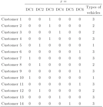
The robust Pareto solutions for problem 6 in small scale in 200th iteration by NSACO algorithm are as follows (where number of customers = 14, number of DCs = 6, types of vehicles = 3):
Number of robust Pareto front members = 2. Robust Pareto front:
For the 1st element of Robust Pareto front, depot vector is: y = 1 1 1 1 1 1.
Allocation matrix for the 1st element of Robust Pareto front is shown in Table A.1.
For the 2nd element of robust Pareto front, depot vector is: y = 1 1 1 1 0 1.
Allocation matrix for the 2nd element of Robust Pareto front is shown in Table A.2.
Final objective values:
For the 1st element of robust Pareto front, objective values are:
Total cost = 1.1391e+006, Transit time = 3.2200.
For the 2nd element of robust Pareto front, objective values are:
Total Cost = 1.1747e+006, Transit Time = 3.1300.
Table A.1. Allocation matrix for the 1st element of robust Pareto front.
x =
DC1 DC2 DC3 DC4 DC5 DC6 Types of vehicles
Customer 1 0 0 1 0 0 0 3
Customer 2 0 0 1 0 0 0 2
Customer 3 0 0 0 1 0 0 2
Customer 4 0 0 1 0 0 0 3
Customer 5 0 1 0 0 0 0 1
Customer 6 0 0 0 0 0 1 3
Customer 7 1 0 0 0 0 0 3
Customer 8 0 1 0 0 0 0 2
Customer 9 0 0 0 0 0 1 3
Customer 10 1 0 0 0 0 0 1
Customer 11 0 0 0 0 0 1 3
Customer 12 0 1 0 0 0 0 2
Customer 13 0 0 0 1 0 0 3
Customer 14 0 0 0 0 1 0 3
Table A.2. Allocation matrix for the 2nd element of robust Pareto front.
x =
DC1 DC2 DC3 DC4 DC5 DC6 Types of vehicles
Customer 1 0 0 0 0 0 1 3
Customer 2 0 0 1 0 0 0 1
Customer 3 0 0 0 1 0 0 3
Customer 4 0 1 0 0 0 0 2
Customer 5 0 0 1 0 0 0 3
Customer 6 0 1 0 0 0 0 3
Customer 7 0 0 0 0 0 0 1
Customer 8 0 0 0 0 0 1 3
Customer 9 0 0 1 0 0 0 3
Customer 10 1 0 0 0 0 0 2
Customer 11 0 0 0 0 0 1 3
Customer 12 1 0 0 0 0 0 2
Customer 13 0 0 1 0 0 0 3
Customer 14 1 0 0 0 0 0 3
Biographies
Jafar Bagherinejad received his PhD degree from Bradford University, UK (1997), and is an Associate Professor of the Industrial Engineering Department, Faculty of Engineering and Technology, Alzahra Uni-versity, Tehran, Iran. His research interest areas are location-allocation problems including queuing models,
queueing systems, project management and control, especially on scheduling problems, quality manage-ment, control and quality systems and innovation and technology engineering and engineering manage-ment. His professional and teaching experiences are: The Dean of Engineering and Technology Faculty, Alzahra University, 2000-2007, and the head of In-dustrial Engineering Department, 2011-2015; Teaching at Industrial Engineering Department, since 2000, for undergraduate and postgraduate students in the
Industrial Engineering and Information Technology Management programs. Further, he has several pa-pers published in the national and international Jour-nals.
Mina Dehghani received her both BS and MS degrees in Industrial Engineering from Alzahra University, Tehran, Iran in 2011 and 2013, respectively. Her main research interests include: optimization, location, meta-heuristics algorithms and SCM.