ORACLE 10g Lab Guide

(1)

(2)

Introduction to the ORACLE 10g Lab Guide

This lab guide is designed to provide examples and exercises in the fundamentals of SQL within the ORACLE 10g environment. The objective is not to develop full blown

applications but to illustrate the concepts of SQL using simple examples. The lab guide has been divided up into 10 sessions. Each one comprises of examples, tasks and

exercises about a particular concept in SQL and how it is implemented in ORACLE 10g. On completion of this 10 week lab guide you will be able to:

• Create a simple relational database in ORACLE 10g

• Insert, update and delete data the tables

• Create queries using basic and advanced SELECT statements

• Perform join operations on relational tables

• Apply set operators

• Use aggregate functions in SQL

• Write subqueries

• Create views of the database

This lab guide assumes that you know how to perform basic operations in the Microsoft Windows environment. Therefore, you should know what a folder is, how to maximize or minimize a folder, how to create a folder, how to select a file, how you maximize and minimize windows, what clicking and double-clicking indicate, how you create a folder, how you drag, how to use drag and drop, how you save a file, and so on.

(4)

The lab guide has been designed on ORACLE 10g version 10.2.0.1.0 running on

Windows XP Professional. Before starting this guide, you must log on to your ORACLE RDBMS, using a user IDand a password created by your database administrator. How you connect to the ORACLE database depends on how the ORACLE software was installed on your server and on the access paths and methods defined and managed by the database administrator. Follow the instructions provided by your instructor, College or University.

(5)

Lab 1: The ORACLE 10g DBMS interfaces

The learning objectives of this lab are to:

• Learn how to use two standard ORACLE 10g interfaces to SQL

• Learn the basic command line SQL editing commands

• Load and run database scripts in the two interfaces

1.1 Introduction

The ORACLE 10g DBMS has a number of interfaces for executing SQL queries. The most basic interface, known as the ORACLE SQL *Plus interface, is used to directly execute SQL commands such as those you will have learnt about in Chapter 8, Introduction to Structured Query Language. An example of the ORACLE SQL *Plus interface can be seen in Figure 1.

(6)

Figure 1: The ORACLE SQL *Plus interface

In Figure 1, the following SQL query has been entered at the command line: SELECT P_CODE, P_DESCRIPT, P_INDATE, P_SALECODE

FROM PRODUCT;

Notice that a semi-colon (;) is needed at the end of the SQL query. This ends the SQL

statement and when the enter key is pressed the query is executed. The results are displayed immediately below the query.

(7)

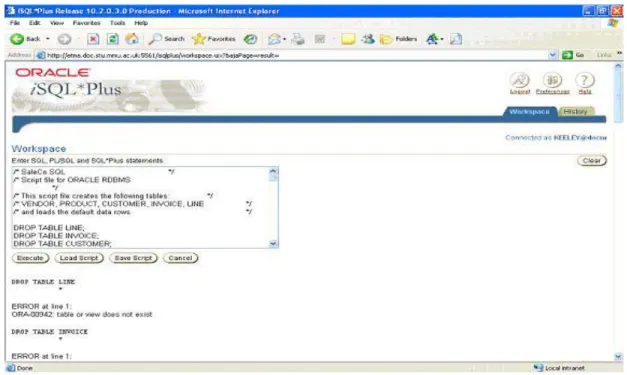
main benefit of this interface is that it allows online editing of SQL statements to take place easily. You can also do some simple formatting of the query output. Figure 2 shows the ORACLE 10g iSQL *Plus interface.

Figure 2: The ORACLE iSQL *Plus interface

Which interface you use to do these lab exercises depends on how the ORACLE software was installed on your server and on the access paths and methods defined and managed by your database administrator. Follow the instructions provided by your instructor, College or University in order to start up and log into the ORACLE database before commencing any of the tasks, examples and exercises in this lab guide.

(8)

1.3 Creating Databases from script files

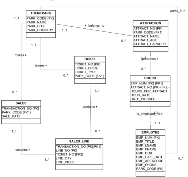
In this section you will learn how to create a small database called SaleCo from a script file. The SQL script file SaleCo.sql for creating the tables and loading the data in the database are located in the Student CD-ROM companion. The database design for the SaleCo database is shown in Figure 3 in the form of an Entity Relationship Diagram (ERD).

Figure 3: The SaleCo Database ERD

(9)

If you are using the command line ORACLE SQL *Plus interface and your own working directory is H:\ORACLE, then in order to create the ORACLE tables you would enter the following command:

SQL>@h:\Oracle\SaleCo

This will load and execute the script to create the SaleCo database. Notice that prompts will indicate that tables are being created and data added as shown in Figure 4.

Figure 4 Creating the SaleCo database using the command line ORACLE SQL *Plus interface

(10)

3. Then click the LOAD button

4. When the script has been loaded click the EXECUTE button

This script will display several messages stating that the different tables required have been created and that test has been inserted into them. The results can be seen in Figure 5.

(11)

1.4 Command Line SQL Editing Commands

Throughout this guide we will be using the command line ORACLE SQL *Plus interface. A number of SQL commands exist in order to perform simple editing of SQL statements that are entered. SQL editing commands are entered one line at a time and are not stored in the SQL buffer. A list of SQL commands that you should become familiar with are

Note

Chapter 8, Introduction to Structured Query Language and Chapter 9, Advanced SQL should be studied alongside this lab guide. You can study Appendix A, Designing Databases with Visio Professional: A Tutorial, if you want to create the database design shown in Figure 3.

Note

When you run the script for the first time you will see some error messages on the screen. These error messages are caused by the script attempting to DROP the database tables before they have been created. Including SQL DROP commands in a script that is being used for development is a good idea to ensure that if changes are made to the database structure, all tables are then recreated to reflect this change. If you run the script again you will see that the error messages no longer appear.

(12)

Command Description

A [APPEND] text Adds text to the end of the current line

C [HANGE] / old / new Changes old text to new text in the current line

C [HANGE] / text / Deletes text from the current line

CL [EAR] BUFF [ER] Deletes all lines from the SQL buffer

DEL Deletes current line

DEL n Deletes line n

DEL m n Deletes lines m to n inclusive

I [NPUT] Inserts an indefinite number of lines

I [INPUT] text Inserts a line consisting of text

L [IST] Lists all lines in the SQL buffer

L [IST] n Lists one line specified by n

L [IST] m n Lists a range of lines m to n inclusive

R [UN] Displays and runs the current SQL statement in the buffer

n Specified the line to make the current line

n text Replaces line n with text

0 text Inserts a line before line 1

SAVE <filename> Save stores the current contents of the SQL buffer in a file

START The start command is used to run a script

(13)

Task 1.2 Enter in the following SQL statement at the SQL command prompt:

Task 1.3 Listing commands in the buffer.

Enter the list command at the SQL prompt as shown below:

Notice that the semicolon you entered at the end of the SELECT command is not listed. This semicolon is necessary to indicate the end of the command when you enter it, but it is not part of the SQL command and SQL*Plus does not store it in the SQL buffer.

Task 1.4 Correcting an error in command line. Note

It is important to note that these commands are not available in iSQLPlus. If you are

using the iSQLPlus interface you will not be able to complete the following tasks and

exercises in the rest of Lab 1 and you should proceed to Lab 2.

SQL>list

SQL> SELECT CUS_CODE, CUS_LNAME, CUS_FNAME, CUS_AREACODE, CUS_BALANCE 2 FROM CUSTOMER

3* WHERE CUS_BALANCE > 0

SQL> SELECT CUS_CODE, CUS_LNAME, CUS_FNAME, CUS_PHONE, CUS_BALANCE FROM CUSTOMER

(14)

Suppose you try to select the CUS_AREACODE column but mistakenly enter it as CU_AREACODE. Enter the following command, purposely misspelling

CUS_AREACODE in the first line as shown below:

You see this message on your screen:

Examine the error message; it indicates an invalid column name in line 1 of the query. The asterisk shows the point of error – the miss-typed column CUS_AREACODE. Instead of re-entering the entire command, you can correct the mistake by editing the command in the buffer. The line containing the error is now the current line. Use the CHANGE command to correct the mistake. This command has three parts, separated by slashes or any other non-alphanumeric character:

• the word CHANGE or the letter C

SQL> SELECT CUS_CODE, CUS_LNAME, CU_AREACODE, CUS_BALANCE FROM CUSTOMER

WHERE CUS_AREACODE =0181;

SELECT CUS_CODE, CUS_LNAME, CU_AREACODE, CUS_BALANCE *

ERROR at line 1:

(15)

The CHANGE command finds the first occurrence in the current line of the character sequence to be changed and changes it to the new sequence. You do not need to use the CHANGE command to re-enter an entire line.

To change CU_AREACODE to CUS_AREACODE, change the line with the CHANGE command as shown below:

The corrected line appears on your screen:

Now that you have corrected the error, you can use the RUN command to run the command again and the correct result is displayed as follows:

CUS_CODE CUS_LNAME CUS_AREACODE CUS_BALANCE

10010 Ramas 0181 0

10012 Smith 0181 345.86

10013 Olowski 0181 536.75

10015 O'Brian 0181 0

10016 Brown 0181 221.19

10017 Williams 0181 768.93

10019 Smith 0181 0

Task 1.5 Adding a new line.

SQL> CHANGE /CU_AREACODE/CUS_AREACODE

(16)

line at the beginning of the buffer and all lines are renumbered starting at 1. Suppose you want to add a fourth line to the SQL query you have just modified in task 1.4. Since line 3 is already the current line, enter INPUT and press Return. SQL*Plus then prompts you for the new line:

Enter the new line and then press Return.

SQL*Plus prompts you again for a new line numbered ‘5’. Press Return again to indicate that you will not enter any more lines, and then use RUN to verify and re-run the query.

Task 1.6 Appending text to a line.

To add text to the end of a line in the buffer, use the APPEND command. Use the LIST command (or the line number) to list the line you want to change.

Enter APPEND followed by the text you want to add. If the text you want to add begins with a blank, separate the word APPEND from the first character of the text by two blanks: one to separate APPEND from the text; and one to go into the buffer with the text.

For example, to append a space and the clause DESC to line 4 of the current query, you should first list the line you want to amend:

SQL> INPUT 4

(17)

Then, enter the following command (be sure to type two spaces between APPEND and DESC):

Type RUN to verify the query and obtain the results shown below:

CUS_CODE

CUS_LNAME CUS_AREACODE CUS_BALANCE

10017 Williams 0181 768.93

10013 Olowski 0181 536.75

10012 Smith 0181 345.86

10016 Brown 0181 221.19

10019 Smith 0181 0

10010 Ramas 0181 0

10015 O'Brian 0181 0

Task 1.7 Deleting Lines.

Use the DEL command to delete lines in the SQL buffer. Enter DEL, specifying the line numbers you want to delete. Suppose you want to delete the current line to the last line inclusive. Use the DEL command as shown:

DEL makes the following line of the buffer (if any) the current line.

SQL> APPEND DESC

4* ORDER BY CUS_BALANCE DESC

(18)

The START command retrieves a script and runs the commands it contains. Use START to run a script containing SQL commands and SQL*Plus commands. Type the START command and then the name of the file like this:

START file_name

ORACLE 10g, SQL*Plus assumes the file has a .SQL extension by default. To retrieve and run the command stored in SALES.SQL, enter the following:

SQL*Plus will then run the commands in the file SALES and displays the results of the commands on your screen, formatting the query results according to the SQL*Plus commands in the file. You can also use the “at” sign (@) command to run a script like this:

Both the @ and @@ commands list and run the commands in the specified script in the same manner as START. To see the commands as SQL*Plus "enters" them, you can SET

. The ECHO system variable controls the listing of the commands in scripts

SQL> SAVE SALES.sql

SQL> START SALES

(19)

the listing. START, @ and @@ leave the last SQL command or PL/SQL block of the script in the buffer.

1.5 Exercises

Answer the following questions.

E1.1 Fill in the blanks.

When appending text to a line:

1) Use the [ ] command to display the line you want to change. 2) Enter [ ] followed by the text you want to add.

E1.2 You type in the following SQL query below:

You see this message on your screen:

Which SQL command would you use to correct this error?

E1.3 Is the following statement correct?

SQL> SELECT EMP_AME, DATE_HIRED, FROM EMPLOYEE WHERE DATE_HIRED = '01-MAY-05';

SELECT EMP_AME, DATE_HIRED *

ERROR at line 1:

ORA-00904: invalid column name

(20)

You then type the following SQL command:

Is the following output correct?

E1.5 Fill in the blanks.

1. To insert a new line after the current line use the [ ] command. 2. To insert a line before line 1 enter a [ ] and follow with the text.

3. SQL*Plus then inserts the line at the beginning of the [ ] and all lines are renumbered starting at 1.

E1.6 Are the following statements True or False?

1. The @ command can be used to load and run SQL scripts in command line. 2. The LIST command shows all lines in the SQL buffer.

E1.7 Fill in blanks.

1. The CHANGE command finds the [ ] occurrence in the [ ] line of the character sequence to be changed and changes it to the new sequence.

SQL> SELECT EMP_NO, EMP_LNAME, DOB, DATE_HIRED 2 FROM EMPLOYEE

3 WHERE SALARY>16000;

SQL> L 1

(21)

Lab 2: Creating a database from a script file

• Create table structures using ORACLE data types

• Apply SQL constraints to ORACLE tables

• Create a simple index

2.1 Introduction

In this section you will learn how to create a small database called Theme Park from the ERD shown in Figure 4. This will involve you creating the table structures in ORACLE using the CREATE TABLE command. In order to do this, appropriate data types will need to be selected from the data dictionary for each table structure, along with any constraints that have been imposed (e.g. primary and foreign key). Converting any ER model to a set of tables in a database requires following specific rules that govern the conversion. The application of those rules requires an understanding of the effects of updates and deletions on the tables in the database. You can read more about these rules in Chapter 8, Introduction to Structure red Query Language, and Appendix D, Converting an ER Model into a Database Structure.

2.2 The Theme Park Database

Figure 6 shows the ERD for the Theme Park database, which will be used throughout this lab guide.

(22)

Figure 6: The Theme Park Database ERD

Table 2.1 Shows the Data Dictionary for the Theme Park database, which will be used to create each table structure.

(23)

Table 2.1 Data Dictionary for the Theme Park Database

Table Name

Attribute Name

Contents Data Type Format Range

Require d PK or FK FK Referenced Table

THEMEPARK PARK_CODE Park code VARCHAR2(10) XXXXXXXX NA Y PK

PARK_NAME Park Name VARCHAR

2(35)

XXXXXXXX NA Y

PARK_CITY City VARCHAR

2(50)

NA Y

PARK_COUNTR

Y

Country CHAR(2) XX NA Y

EMPLOYEE EMP_NUM Employee

number

NUMBER(4) ## 0000 – 9999 Y PK

EMP_TITLE Employee

title

VARCHAR2(4) XXXX NA N

EMP_LNAME Last name VARCHAR2(15) XXXXXXXX NA Y

EMP_FNAME First Name VARCHAR2(15) XXXXXXXX NA Y

EMP_DOB Date of

Birth

DATE DD-MON-YY NA Y

EMP_HIRE_DAT

E

Hire date DATE DD-MON-YY NA Y

EMP_AREACOD E

Area code VARCHAR2(4) XXXX NA Y

(24)

TICKET TICKET_NO Ticket

number

NUMBER(10) ########## NA Y

TICKET_PRICE Price NUMBER(4,2) ####.## 0.00 – 0000.00

TICKET_TYPE Type of

ticket VARCHAR2(10) XXXXXXXX XX Adult, Child,Senio r,Other

PARK_CODE Park code VARCHAR2(10) XXXXXXXX NA Y FK THEMEPA

RK

ATTRACTION ATTRACT_NO Attraction number

NUMBER(10) ########## N/A Y PK

PARK_CODE Park code VARCHAR2(10) XXXXXXXX NA Y FK THEMEPA

RK

ATTRACT_NAM

E

Name VARCHAR2(35) XXXXXXX N/A N

ATTRACT_AGE Age NUMBER(3) ### Default 0 Y

ATTRACT_CAP ACITY

Capacity NUMBER(3) ### N/A Y

HOURS EMP_NUM Employee

number

NUMBER(4) ## 0000 – 9999 Y PK /

FK

EMPLOYEE

ATTRACT_NO Attraction

number

NUMBER(10) ########## N/A Y PK /

FK ATTRACTI ON HOURS_PER_AT TRACT Number of hours

NUMBER(2) ## N/A Y

(25)

SALES TRANSACTION_

NO

Transaction

No

NUMBER ########### N/A Y PK

PARK_CODE Park code VARCHAR2(10) XXXXXXXX NA Y FK THEMEPA RK

SALE_DATE Date of Sale DATE DD-MON-YY SYSDATE Y

SALESLINE TRANSACTION_

NO

Transaction

No

NUMBER ########### N/A Y PK /

FK

SALES

LINE_NO Line

number

NUMBER(2) ## N/A Y

TICKET_NO Ticket

number

NUMBER(10) ########## NA Y FK TICKET

LINE_QTY Quantity NUMBER(4) #### N/A Y

LINE_PRICE Price of line NUMBER(9,2) #########.## N/A Y

2.3 Creating the Table Structures

Use the following SQL commands to create the table structures for the Theme Park database. Enter each one separately to ensure that you have no errors. Successful table creation will prompt ORACLE to say “Table Created”. It is useful to store each correct table structure in a script file, in case the entire database needs to be recreated again at a later date. You can use a simple text editor such as notepad in order to do this. Save the file as themepark.sql. Note that the table-creating SQL commands used in this example are based on the data dictionary shown in Table 2.1.

As you examine each of the SQL table-creating command sequences in the following tasks, note the following features:

(26)

• The NOT NULL specifications for the attributes ensure that a data entry will be

made. When it is crucial to have the data available, the NOT NULL specification will not allow the end user to leave the attribute empty (with no data entry at all).

• The UNIQUE specification creates a unique index in the respective attribute. Use

it to avoid duplicated values in a column.

• The primary key attributes contain both a NOT NULL and a UNIQUE

specification. Those specifications enforce the entity integrity requirements. If the NOT NULL and UNIQUE specifications are not supported, use PRIMARY KEY without the specifications.

• The entire table definition is enclosed in parentheses. A comma is used to separate

each table element (attributes, primary key and foreign key) definition.

• The DEFAULT constraint is used to assign a value to an attribute when a new row

is added to the table. The end user may, of course, enter a value other than the default value.

• The CHECK constraint is used to validate data when an attribute value is entered.

The CHECK constraint does precisely what its name suggests: it checks to see that a specified condition exists. If the CHECK constraint is met for the specified attribute (that is, the condition is true), the data are accepted for that attribute. If the condition is found to be false, an error message is generated and the data are not accepted.

(27)

Task 2.1 Enter the following SQL command to create the THEMEPARK table.

CREATE TABLE THEMEPARK (

PARK_CODE VARCHAR2(10) PRIMARY KEY,

PARK_NAME VARCHAR2(35) NOT NULL,

PARK_CITY VARCHAR2(50) NOT NULL,

PARK_COUNTRY CHAR(2) NOT NULL);

Notice that when you create the THEMEPARK table structure you set the stage for the enforcement of entity integrity rules by using:

PARK_CODE VARCHAR2(10) PRIMARY KEY,

As you create this structure, also notice that the NOT NULL constraint is used to ensure that the columns PARK_NAME, PARK_CITY and PARK_COUNTRY do not accept nulls.

Remember to store this CREATE TABLE structure in your themepark.sq script.

2.3.2 Creating the EMPLOYEE TABLE

Task 2.2 Enter the following SQL command to create the EMPLOYEE table.

CREATE TABLE EMPLOYEE (

EMP_NUM NUMBER(4) PRIMARY KEY,

EMP_TITLE VARCHAR2(4),

(28)

EMP_HIRE_DATE DATE DEFAULT SYSDATE, EMP_AREA_CODE VARCHAR2(4) NOT NULL,

EMP_PHONE VARCHAR2(12) NOT NULL,

CONSTRAINT FK_EMP_PARK FOREIGN KEY(PARK_CODE) REFERENCES

THEMEPARK(PARK_CODE));

As you look at the CREATE TABLE sequence, note that referential integrity has been enforced by specifying a constraint called FKP_EMP_PARK. This foreign key constraint definition ensures that you cannot delete a Theme Park from the THEMEPARK table if at least one employee row references that Theme Park. The ORACLE RDBMS will

automatically enforce referential integrity for foreign keys. This ensures that you cannot have an invalid entry in the foreign key column. In this example the employee’s hire date is set to the SYSDATE using the DEFAULT constraint, so when a new employee record is created the SYSDATE function always returns today’s date.

2.3.3 Creating the TICKET TABLE

Task 2.3 Enter the following SQL command to create the TICKET table.

CREATE TABLE TICKET (

(29)

PARK_CODE VARCHAR2(10),

CONSTRAINT CK_TICKET_TYPE CHECK (TICKET_TYPE IN('Adult','Child','Senior','Other')),

CONSTRAINT FK_TICKET_PARK FOREIGN KEY(PARK_CODE)

REFERENCES THEMEPARK(PARK_CODE))

As you create the TICKET table, notice that a number of constraints have been applied. For example, a CHECK constraint called CK_TICKET_TYPE is used to validate that the ticket type is 'Adult', 'Child', 'Senior' or 'Other'.

2.3.4 Creating the ATTRACTION TABLE

Task 2.4 Enter the following SQL command to create the ATTRACTION table.

CREATE TABLE ATTRACTION (

ATTRACT_NO NUMBER(10) PRIMARY KEY,

ATTRACT_NAME VARCHAR2(35),

ATTRACT_AGE NUMBER(3) DEFAULT 0 NOT NULL,

ATTRACT_CAPACITY NUMBER(3) NOT NULL,

CONSTRAINT FK_ATTRACT_PARK FOREIGN KEY(PARK_CODE)

(30)

2.3.5 Creating the HOURS TABLE

Task 2.5 Enter the following SQL command to create the HOURS table.

CREATE TABLE HOURS (

EMP_NUM NUMBER(4),

ATTRACT_NO NUMBER(10),

HOURS_PER_ATTRACT NUMBER(2) NOT NULL,

HOUR_RATE NUMBER(4,2) NOT NULL,

DATE_WORKED DATE NOT NULL,

CONSTRAINT PK_HOURS PRIMARY KEY(EMP_NUM,

ATTRACT_NO, DATE_WORKED),

CONSTRAINT FK_HOURS_EMP FOREIGN KEY (EMP_NUM) REFERENCES EMPLOYEE(EMP_NUM),

CONSTRAINT FK_HOURS_ATTRACT FOREIGN KEY (ATTRACT_NO) REFERENCES ATTRACTION(ATTRACT_NO));

As you create the HOURS table, notice that the HOURS table contains FOREIGN KEYS to both the ATTRACTION and the EMPLOYEE’s table.

(31)

CREATE TABLE SALES (

TRANSACTION_NO NUMBER PRIMARY KEY,

SALE_DATE DATE DEFAULT SYSDATE NOT NULL,

CONSTRAINT FK_SALES_PARK FOREIGN KEY(PARK_CODE)

REFERENCES THEMEPARK(PARK_CODE) ON DELETE CASCADE,

CONSTRAINT SALE_CK1 CHECK (SALE_DATE >

TO_DATE('01-JAN-2005','DD-MON-YYYY')));

As you create the SALES table, look closely at the SALE_CK1 CHECK constraint. Can you describe the purpose of this constraint?

2.3.7 Creating the SALESLINE TABLE

Task 2.7 Enter the following SQL command to create the SALES_LINE table.

CREATE TABLE SALES_LINE ( TRANSACTION_NO NUMBER,

LINE_NO NUMBER(2,0) NOT NULL,

(32)

CONSTRAINT PK_SALES_LINE PRIMARY KEY (TRANSACTION_NO,LINE_NO),

CONSTRAINT FK_SALES_LINE_SALES FOREIGN KEY (TRANSACTION_NO) REFERENCES SALES ON DELETE CASCADE,

CONSTRAINT FK_SALES_LINE_TICKET FOREIGN KEY (TICKET_NO) REFERENCES TICKET(TICKET_NO));

As you create the SALES_LINE table, examine the constraint called

FK_SALES_LINE_SALES. What is the purpose of ON DELETE CASCADE? Remember to store this CREATE TABLE structure in your themepark.sq script.

2.4. Creating Indexes

You learned in Chapter 3, The Relational Database Model, that indexes can be used to improve the efficiency of searches and to avoid duplicate column values. Using the

CREATE INDEX command, SQL indexes can be created on the basis of any selected

attribute. For example, based on the attribute SALE_DATE stored in the SALES table, the following command creates an index named SALE_DATE_INDEX:

CREATE INDEX SALE_DATE_INDEX ON SALES(SALE_DATE);

Task 2.8 Create the SALE_DATE_INDEX shown above and add the CREATE INDEX

(33)

The DROP TABLE command permanently deletes a table (and thus its data) from the

database schema. When you write a script file to create a database schema, it is useful to add DROP TABLE commands at the start of the file. If you need to amend the table structures in any way, just one script can then be run to re-create all the database structures. Primary and foreign key constraints control the order in which you drop the tables – generally you drop in the reverse order of creation. The DROP commands for the Theme Park database are:

DROP TABLE SALES_LINE; DROP TABLE SALES;

DROP TABLE HOURS;

DROP TABLE ATTRACTION; DROP TABLE TICKET; DROP TABLE EMPLOYEE; DROP TABLE THEMEPARK;

Task 2.9. Add the DROP commands to the start of your script file and then run the

themepark.sql script.

2.4 Display a table’s structure

The command DESCRIBE is used to display the structure of an individual table. To see the structure of the THEMEPARK table you would enter the command

(34)

Task 2.10 Use the DESCRIBE command to view the structure of the other database

tables that you have created in this lab.

2.5 Listing all tables

To list all tables that have been created by yourself you need to access ORACLE’s data dictionary in order to view the metadata. For example, to find out the names of all of the relational tables that you have created, you must type the following query:

SELECT TABLE_NAME FROM USER_TABLES;

Task 2.11 Execute a query which displays all the tables you own and check to see if the

tables you have created in this lab are present.

2.6 Altering the table structure

All changes in the table structure are made by using the ALTER TABLE command, Note

To find out more about data dictionaries in ORACLE DBMS visit the Oracle Technological Network at: http://www.oracle.com/technology/index.html.

(35)

column, and MODIFY enables you to change column characteristics. Most RDBMSs do not allow you to delete a column (unless the column does not contain any values), because such an action may delete crucial data that are used by other tables. The basic syntax to add or modify columns is:

ALTER TABLE tablename

{ADD | MODIFY}( columnname datatype [ {ADD | MODIFY} columnname datatype]);

The ALTER TABLE command can also be used to add table constraints. In those cases, the syntax would be:

ALTER TABLE tablename

ADD constraint [ ADD constraint ] ;

where constraint refers to a constraint definition, e.g. primary or foreign key.

However, when removing a constraint you need to specify the name given to the constraint. That is one reason why you should always name your constraints in your CREATE TABLE or ALTER TABLE statement.

If you wanted to modify the column ATTRACT_CAPACITY in the ATTRACTION table by changing the date characteristics from NUMBER(3) to NUMBER(4), you would execute the following command:

(36)

MODIFY (ATTRACT_CAPACITY NUMBER(4));

You have now reached the end of the first ORACLE lab. The tables that you have created will be used in the rest of this lab guide to explore the use of SQL in ORACLE in more detail.

Note

Some DBMSs impose limitations on when it’s possible to change attribute

characteristics. For example, ORACLE lets you increase (but not decrease) the size of a column. The reason for this restriction is that an attribute modification will affect the integrity of the data in the database. In fact, some attribute changes can be done only when there are no data in any rows for the affected attribute.

You can learn more about altering a table’s structure in Chapter 8, Introduction to Structured Query Language.

(37)

Lab 3: Data Manipulation Commands

The learning objectives for this lab are:

• To know how to insert, update and delete data from within a table • To learn how to retrieve data from a table using the SELECT statement

3.1 Adding Table Rows

SQL requires the use of the INSERT command to enter data into a table. The INSERT

command’s basic syntax looks like this:

INSERT INTO tablename VALUES (value1, value2, ... , valuen).

The order in which you insert data is important. For example, because the TICKET uses its PARK_CODE to reference the THEMEPARK table’s PARK_CODE, an integrity violation will occur if those THEMEPARK table PARK_CODE values don’t yet exist. Therefore, you need to enter the THEMEPARK rows before the TICKET rows.

Complete the following tasks to insert data into the THEMEPARK and TICKET tables:

Task 3.1 Enter the first two rows of data into the THEMEPARK table using the

following SQL insert commands;

INSERT INTO THEMEPARK VALUES ('FR1001','FairyLand','PARIS','FR'); INSERT INTO THEMEPARK VALUES ('UK3452','PleasureLand','STOKE','UK');

(38)

Task 3.2 Enter the following corresponding rows of data into the TICKET table using the

following SQL insert commands.

INSERT INTO TICKET VALUES (13001,18.99,'Child','FR1001'); INSERT INTO TICKET VALUES (13002,34.99,'Adult','FR1001'); INSERT INTO TICKET VALUES (13003,20.99,'Senior','FR1001'); INSERT INTO TICKET VALUES (88567,22.50,'Child','UK3452'); INSERT INTO TICKET VALUES (88568,42.10,'Adult','UK3452'); INSERT INTO TICKET VALUES (89720,10.99,'Senior','UK3452');

Any changes made to the table contents are not physically saved on disk until you close the database, close the program you are using, or use the COMMIT command. The

COMMIT command will permanently save any changes – such as rows added, attributes

modified, and rows deleted – made to any table in the database. Therefore, if you intend to make your changes to the THEMEPARK and TICKET tables permanent, it is a good idea to save those changes by using COMMIT;

Task 3.3 COMMIT the changes to the THEMEPARK and TICKET tables to the

(39)

Task 3.4 Run the script file themeparkdata.sql to insert the rest of the data into the

Theme Park database. This script file is available on the CD-ROM companion. Ensure you COMMIT the changes to the database.

3.2 Retrieving data from a table using the SELECT Statement

In Chapter 8, Introduction to Structured Query Language, you studied the SELECT command. The SELECT command has many optional clauses, but in its simplest can be written as:

SELECT columnlist

FROM tablelist

[WHERE conditionlist ];

Notice that the command must finish with a semicolon and will be executed when the Enter key is pressed at the end of the command.

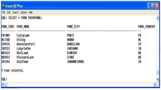
The simplest query involves viewing all columns in one table. To display the details of all Theme Parks in the Theme Park database, type the following:

SELECT *

FROM THEMEPARK;

(40)

Figure 7: Displaying all columns from the CUSTOMER Table

The SELECT command and the FROM clause are necessary for any SQL query, and must always be included so that the DBMS knows which columns we want to display and which table they come from.

Task 3.5. Type in the following examples of the SELECT statement and check your

results with those provided in Figures 8 and 9. In these two examples you are selecting specific columns from a single table.

Example 1

SELECT ATTRACT_NO, ATTRACT_NAME, ATTRACT_CAPACITY FROM ATTRACTION;

Example 2

SELECT EMP_NUM, EMP_LNAME, EMP_FNAME, EMP_HIRE_DATE FROM EMPLOYEE;

(41)

Figure 8: Output for Example 1

Figure 9: Output for Example 2 3.3 Updating table rows

The UPDATE command is used to modify data in a table. The syntax for this command

is:

(42)

For example, if you wanted to change the attraction capacity of the attraction number 10034 from 34 to 38, the primary key, ATTRACT_NO would be used to locate the correct (second) row. You would type:

UPDATE ATTRACTION

SET ATTRACT_CAPACITY = 34

WHERE ATTRACT_NO= 10034;

The output is shown in Figure 10.

Figure 10: Updating the attraction capacity

Note

If more than one attribute is to be updated in the row, separate each attribute with commas.

(43)

Remember, the UPDATE command is a set-oriented operator. Therefore, if you don’t specify a WHERE condition, the UPDATE command will apply the changes to all rows

in the specified table.

Task 3.6 Enter the following SQL UPDATE command to update the age a person can go

on a specific ride in the Theme Park. UPDATE ATTRACTION

SET ATTRACT_AGE = 14;

Confirm the update by using this command to check the ATTRACTION table’s listing:

SELECT * FROM ATTRACTION;

Notice that all the values of ATTRACT_AGE have the same value.

3.4 Restoring table contents

Suppose you decide you have made a mistake in updating the attraction age to be the same for all attractions within the Theme Park. Assuming you have not yet used the COMMIT command to store the changes permanently in the database, you can restore the database to its previous condition with the ROLLBACK command. ROLLBACK undoes

any changes and brings the data back to the values that existed before the changes were made.

(44)

ROLLBACK;

and press Enter. Use the SELECT statement again to see that the ROLLBACK did, in fact, restore the data to their original values.

3.5 Deleting table rows

It is easy to delete a table row using the DELETE statement. The syntax is:

DELETE FROM tablename

For example, if you want to delete a specific Theme Park from the THEMEPARK table you could use the PARK_CODE as shown in the following SQL command:

DELETE FROM THEMEPARK

WHERE PARK_CODE = ′ SW2323′;

In this example, the primary key value lets SQL find the exact record to be deleted. However, deletions are not limited to a primary key match; any attribute may be used. If you do not specify a WHERE condition, all rows from the specified table will be

deleted!

Note

For more information about ROLLBACK, See section 8.3.5, Restoring Table Contents in Chapter 8, Introduction to Structured Query Language.

(45)

3.6 Inserting Table rows with a subquery

Subqueries are often used to add multiple rows to a table, using another table as the source of the data. The syntax for the INSERT statement is:

INSERT INTO tablename SELECT columnlist FROM tablename;

In that case, the INSERT statement uses a SELECT subquery. A subquery, also known

as a nested query or an inner query, is a query that is embedded (or nested) inside another query. The inner query is always executed first by the RDBMS. Given the previous SQL statement, the INSERT portion represents the outer query and the SELECT portion represents the inner query, or subquery.

Task 3.8 Use the following steps to populate your EMPLOYEE table.

• Run the script emp_copy.sql which is available on the accompanying CD-ROM. This script creates a table called EMP_COPY, which we will populate using data from the EMPLOYEE table in the THEMEPARK database.

• Add the rows to EMP_COPY table by copying all rows from EMPLOYEE. INSERT INTO EMP_COPY SELECT * FROM EMPLOYEE;

Note

If you make a mistake while working through this lab, use the themepark.sql script to re-create the database schema and insert the sample data.

(46)

If you followed those steps correctly, you now have the EMPLOYEE table populated with the data that will be used in the remaining sections of this lab guide.

3.7 Exercises

E3.1 Load and run the script park_copy.sql which creates the PARK_COPY table.

E3.2 Describe the PARK_COPY and THEMEPARK tables and notice that they are

different.

E3.3 Write a subquery to populate the fields PARK_CODE, PARK_NAME and

PARK_COUNTRY in the PARK_COPY using data from the THEMEPARK table. Display the contents of the PARK_COPY table.

E3.4 Update the AREA_CODE and PARK_PHONE fields in the PARK_COPY table

with the following values.

PARK_CODE PARK_AREA_CODE PARK_PHONE

FR1001 5678 223-556

UK3452 0181 678-789

ZA1342 8789 797-121

E3.5 Add the following new Theme Parks to the PARK_COPY TABLE.

(47)

(48)

Lab 4: Basic SELECT statements

• Use arithmetic operators in SQL statements

• Select rows from a table with conditional restrictions

• Apply logical operators to have multiple conditions

4.1 Using Arithmetic operators in SQL Statements

SQL commands are often used in conjunction with arithmetic operators. As you perform mathematical operations on attributes, remember the rules of precedence. As the name suggests, the rules of precedence are the rules that establish the order in which

computations are completed. For example, note the order of the following computational sequence:

1. Perform operations within parentheses 2. Perform power operations

3. Perform multiplications and divisions 4. Perform additions and subtractions

Task 4.1 Suppose the owners of all the Theme Parks wanted to compare the current

(49)

FROM TICKET;

The output for this query is shown in Figure 11. The ROUND function is used to ensure the result is displayed to two decimal places.

Figure 11: Output showing 10% increase in ticket prices

You will see in Figure 11, that the last column is named after the arithmetic expression in the query. To rename the column heading, a column alias needs to be used. Modify the query as follows and note that the name of the heading has changed to

PRICE_INCREASE when you execute the following query.

SELECT PARK_CODE, TICKET_NO, TICKET_TYPE, TICKET_PRICE, TICKET_PRICE + ROUND((TICKET_PRICE *0.1),2) PRICE_INCREASE FROM TICKET;

(50)

4.2 Selecting rows with conditional restrictions

Numerous conditional restrictions can be placed on the selected table contents in the WHERE clause of the SELECT statement. For example, the comparison operators shown in Table 1 can be used to restrict output.

Table 1 Comparison Operators

SYMBOL MEANING

= Equal to

< Less than

<= Less than or equal to

> Greater than

>= Greater than or equal to

<> or != Not equal to

Note

When dealing with column names that require spaces, the optional keyword AS can be used. For example:

SELECT PARK_CODE, TICKET_NO, TICKET_TYPE, TICKET_PRICE, TICKET_PRICE + ROUND((TICKET_PRICE *0.1),2) AS

“PRICE INCREASE” FROM TICKET;

(51)

LIKE Used to check if an attribute value matches a given string pattern IS NULL / IS NOT NULL Used to check if an attribute is NULL / is not NULL

We will now explore some of these conditional operators using examples.

Greater than

The following example uses the greater than operator to display the Theme Park code, ticket price and ticket type of all tickets where the ticket price is greater than €20.00.

SELECT PARK_CODE, TICKET_TYPE, TICKET_PRICE FROM TICKET

WHERE TICKET_PRICE > 20; The output is shown in Figure 12.

(52)

Task 4.3 Modify the query you have just executed to display tickets that are less than

€30.00.

Character comparisons

Comparison operators may even be used to place restrictions on character-based attributes.

Task 4.4 Execute the following query which produces a list of all rows in which the

PARK_CODE is alphabetically less than UK2262. (Because the ASCII code value for the letter B is greater than the value of the letter A, it follows that A is less than B.) The

output will be generated as shown in Figure 13.

SELECT PARK_CODE, PARK_NAME, PARK_COUNTRY

FROM THEMEPARK

(53)

BETWEEN

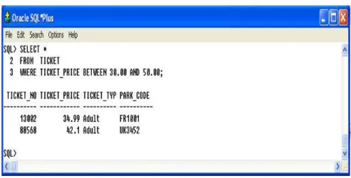
The operator BETWEEN may be used to check whether an attribute value is within a range of values. For example, if you want to see a listing for all tickets whose prices are between €30 and €50, use the following command sequence:

SELECT *

FROM TICKET

WHERE TICKET_PRICE BETWEEN 30.00 AND 50.00;

Figure 14 shows the output you should see for this query.

Figure 14: Displaying ticket prices BETWEEN two values

Task 4.5 Write a query which displays the employee number, attraction no., the hours

worked per attraction and the date worked where the hours worked per attraction is between 5 and 10. Hint: You will need to select data from the HOURS table. The output for the query is shown in Figure 15.

(54)

Figure 15: Output for Task 4.5 IN

The IN operator is used to test for values which are in a list. The following query finds only the rows in the SALES_LINE table that match up to a specific sales transaction. i.e. TRANSACTION_NO is either 12781 or 67593.

SELECT *

FROM SALES_LINE

WHERE TRANSACTION_NO IN (12781, 67593);

(55)

Figure 16: Selecting rows using the IN command

Task 4.6 Write a query to display all tickets that are of type Senior or Child. Hint: Use

the TICKET table. The output you should see is shown in Figure 17.

Figure 17: Output for Task 4.5 LIKE

The LIKE operator is used to find patterns within string attributes. Standard SQL allows you to use the percent sign (%) and underscore (_) wildcard characters to make matches when the entire string is not known. % means any and all following characters are eligible

while _ means any one character may be substituted for the underscore.

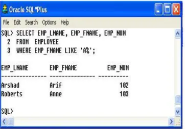
Task 4.7 Enter the following query which finds all EMPLOYEE rows whose first names

begin with the letter A.

(56)

WHERE EMP_FNAME LIKE ′A%′;

Figure 18 shows the output you should see for this query.

Figure 18: Query using the LIKE command

Task 4.8 Write a query which finds all Theme Parks that have a name ending in “Land”.

(57)

NULL and IS NULL

IS NULL is used to check for a null attribute value. In the following example the query lists all attractions that do not have an attraction name assigned (ATTRACT_NAME is null). The query could be written as:

SELECT *

FROM ATTRACTION

WHERE ATTRACT_NAME IS NULL;

The output for this query is shown in Figure 20.

Figure 20: Listing all Attractions with no name

Logical Operators

SQL allows you to have multiple conditions in a query through the use of logical

operators: AND, OR and NOT. ORACLE SQL precedence rules give NOT as the highest precedence, followed by AND, and then followed by OR. However, you are strongly

(58)

AND

This logical AND connective is used to set up a query where there are two conditions which must be met for the query to return the required row(s). The following query displays the employee number (EMP_NUM) and the attraction number

(ATTRACT_NUM) for which the numbers of hours worked (HOURS_PER_ATTRACT) by the employee is greater than 3 and the date worked (DATE_WORKED) is after 18th May 2007.

SELECT EMP_NUM, ATTRACT_NO

FROM HOURS

WHERE HOURS_PER_ATTRACT > 3

AND DATE_WORKED > '18-MAY-07';

(59)

Task 4.9 Enter the query above and check you results with those shown in Figure 21.

Task 4.10 Write a query which displays the details of all attractions which are suitable

for children aged 10 or under and have a capacity of less than 100. You should not

display any information for attractions which currently have no name. Your output should correspond to that shown in Figure 22.

Figure 22: Query results for Task 4.10

OR

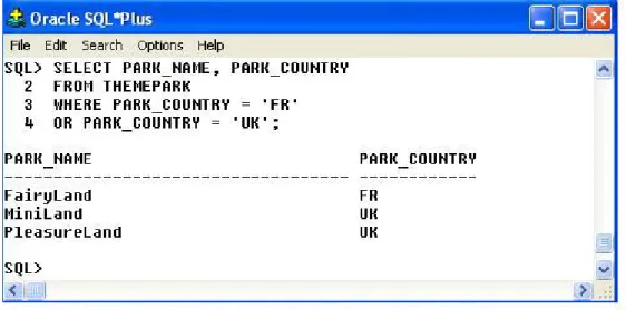
If you wanted to list the names and countries of all Theme Parks in the UK or France you would write the following query.

SELECT PARK_NAME, PARK_COUNTRY FROM THEMEPARK

WHERE PARK_COUNTRY = 'FR' OR PARK_COUNTRY = 'UK';

(60)

Figure 23: Query results using the OR operator

When using AND and OR in the same query it is advisable to use parentheses to make explicit the precedence.

Task 4.11 Test the following query and check your output with that shown in Figure 24.

Can you work out what this query is doing?

SELECT *

FROM ATTRACTION

WHERE (PARK_CODE LIKE ′FR%′

(61)

Figure 24: AND and OR example

NOT

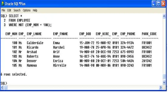
The logical operator NOT is used to negate the result of a conditional expression. If you

want to see a listing of all rows for which EMP_NUM is not 106, the query would look like:

SELECT * FROM EMPLOYEE

WHERE NOT (EMP_NUM = 106);

The results of this query are shown in Figure 25. Note that the condition is enclosed in parentheses; that practice is optional, but it is highly recommended for clarity.

(62)

Figure 25: Listing all employees except EMP_NUM=106

Exercises

E4.1 Write a query to display all Theme Parks except those in the UK.

E4.2 Write a query to display all the sales that occurred on the 19th May 2007.

E4.3 Write a query to display the ticket prices between €20 AND €30.

E4.4 Display all attractions that have a capacity of more that 60 at the Theme Park

FR1001.

(63)

display the ATTRACT_NO, HOUR_RATE and the HOUR_RATE with the 20% increase.

(64)

Lab 5: Advanced SELECT Statements

• Sort the data in the resulting query • Apply SQL aggregate functions

5.1 Sorting Data

The ORDER BY clause is especially useful when the listing order of the query is

important. Although you have the option of declaring the order type – ascending (ASC)

or descending (DESC) – the default order is ascending. For example, if you want to

display all employees listed by EMP_HIRE_DATE in descending order you would write the following query. The output is shown in Figure 26.

SELECT *

FROM EMPLOYEE

(65)

Figure 26: Displaying all employees in descending order of EMP_HIRE_DATE

The ORDER BY command can also be used to produce a cascading order sequence. This is where the query results are ordered against a sequence of attributes.

Task 5.1 Enter the following query, which contains an example of a cascading order

sequence, by ordering the rows in the employee table by the employee’s last then first names.

SELECT *

FROM EMPLOYEE

(66)

It is worth noting that if the ordering column has nulls, they are listed either first or last (depending on the RDBMS). The ORDER BY clause can be used in conjunction with other SQL commands and is listed last in the SELECT command sequence.

Task 5.2 Enter the following query and check your output against the results shown in

Figure 27. Describe in your own words what this query is actually doing.

SELECT TICKET_TYPE, PARK_CODE

FROM TICKET

WHERE (TICKET_PRICE > 15 AND TICKET_TYPE LIKE 'Child') ORDER BY TICKET_NO DESC;

Figure 27: Query results for Task 5.2

(67)

The SQL command DISTINCT is used to produce a list of only those values that are different from one another. For example, to list only the different Theme Parks from within the ATTRACTION table, you would enter the following query.

SELECT DISTINCT(PARK_CODE)

FROM ATTRACTION;

Figure 28 shows that the query only displays the rows that are different.

Figure 28: Displaying DISTINCT rows

5.3 Aggregate Functions

SQL can perform mathematical summaries through the use of aggregate (or group) functions. Aggregate functions return results based on groups of rows. By default, the entire result is treated as one group. Table 3 shows some of the basic aggregate functions.

Table 3 Basic SQL Aggregate Functions

(68)

MIN The minimum attribute value encountered in a given column MAX The maximum attribute value encountered in a given column SUM The sum of all values for a given column

AVG The arithmetic mean (average) for a specified column

COUNT

The COUNT function is used to tally the number of non-null values of an attribute. COUNT can be used in conjunction with the DISTINCT clause. If you wanted to find out how many different Theme Parks contained attractions from the ATTRACTION table you would write the following query

SELECT COUNT(PARK_CODE)

FROM ATTRACTION;

(69)

However, if you wanted to know how many different Theme Parks were in the

ATTRACTION table, you would modify the query as follows (For the output see Figure 30):

SELECT COUNT(DISTINCT(PARK_CODE))

FROM ATTRACTION;

Figure 30: Counting the number of DISTINCT Theme parks in ATTRACTION

Task 5.3 Write a query that displays the number of distinct employees in the HOURS

table. You should label the column “Number of Employees”. Your output should match that shown in Figure 31.

(70)

Figure 31: Query output for Task 5.3

COUNT always returns the number of non-null values in the given column. Another use for the COUNT function is to display the number of rows returned by a query, including the rows that contain rows using the syntax COUNT(*).

Task 5.4 Enter the following two queries and examine their output shown in Figure 32.

Can you explain why the number of rows returned is different?

SELECT COUNT(*)

FROM ATTRACTION;

SELECT COUNT(ATTRACT_NAME)

(71)

Figure 32: Examples of using the COUNT function

MAX and MIN

The MAX and MIN functions are used to find answers to problems such as, “What is the highest and lowest ticket price sold in all Theme Parks?”

Task 5.5 Enter the following query which illustrates the use of the MIN and Max

functions. Check the query results with those shown in Figure 33. SELECT MIN(TICKET_PRICE),max(TICKET_PRICE)

(72)

Figure 33: Examples of using the MIN and MAX functions

SUM and AVG

The SUM function computes the total sum for any specified attribute, using whatever condition(s) you have imposed. The AVG function calculates the arithmetic mean

(average) for a specified attribute. The following query displays the average amount spent on Theme Park tickets per customer (LINE_PRICE) and the total number of tickets purchase (LINE_QTY). Figure 34 shows the output for this query.

SELECT AVG(LINE_PRICE), SUM(LINE_QTY) FROM SALES_LINE;

(73)

Task 5.6 Write a query that displays the average hourly rate that has been paid to all

employees. Hint use the HOURS table. Your query should return €7.03.

Task 5.7 Write a query that displays the average attraction age for all attractions where

the PARK_CODE = ‘UK3452’. Your query should return 7.25 years.

GROUP BY

The GROUP BY clause is generally used when you have attribute columns combined with aggregate functions in the SELECT statement. It is valid only when used in conjunction with one of the SQL aggregate functions, such as COUNT, MIN, MAX, AVG and SUM. The GROUP BY clause appears after the WHERE statement. When using GROUP BY you should include all the attributes that are in the SELECT statement that do not use an aggregate function. The following query displays the minimum and maximum ticket price of all parks. The output is shown in Figure 35. Notice that the query groups only by the PARK_CODE, as no aggregate function is applied to this attribute in the SELECT statement.

SELECT PARK_CODE, MIN(TICKET_PRICE),MAX(TICKET_PRICE)

FROM TICKET

(74)

Figure 35: Displaying minimum and maximum ticket prices for each PARK_CODE

Task 5.7 Enter the query above and check the results against the output shown in Figure

35. What happens if you miss out the GROUP BY clause?

HAVING

The HAVING clause is an extension to the GROUP BY clause and is applied to the output of a GROUP BY operation. Supposing you wanted to list the average ticket price at each Theme Park but wanted to limit the listing to Theme Parks whose average ticket price was greater or equal to €24.99. This can be achieved by the following query whose output is shown in Figure 36.

SELECT PARK_CODE, AVG(TICKET_PRICE)

FROM TICKET

(75)

Figure 36: Example of the HAVING clause

Task 5.8 Using the HOURS table, write a query to display the employee number

(EMP_NUM), the attraction number (ATTRACT-NO) and the average hours worked per attraction (HOURS_PER_ATTRACT), limiting the result to where the average hours worked per attraction is greater or equal to 5. Check your results against those shown in Figure 37.

(76)

E5.1 Write a query to display all unique employees that exist in the HOURS table.

E5.2 Display the employee numbers of all employees and the total number of hours they

have worked.

E5.3. Show the attraction number and the minimum and maximum hourly rate for each

attraction.

E5.4 Write a query to show the transaction numbers and line prices (in the SALES_LINE

table) that are greater than €50.

(77)

Lab 6: JOINING DATABASE TABLES

• Learn how to perform the following types of database joins

o Cross Join o Natural Join o Outer Joins 6.1 Introduction to Joins

The relational join operation merges rows from two or more tables and returns the rows with one of the following conditions:

• Have common values in common columns (natural join)

• Meet a given join condition (equality or inequality)

• Have common values in common columns or have no matching values (outer join)

There are a number of different joins that can be performed. The most common is the natural join. To join tables, you simply enumerate the tables in the FROM clause of the SELECT statement. The DBMS will create the Cartesian product of every table in the FROM clause. However, to get the correct result – that is, a natural join – you must select only the rows in which the common attribute values match. That is done with the

(78)

foreign key in the TICKET table and the primary key in the THEMEPARK table, the link is established on PARK_CODE. It is important to note that when the same attribute name appears in more than one of the joined tables, the source table of the attributes listed in the SELECT command sequence must be defined. To join the THEMEPARK and

TICKET tables you would use the following, which produces the output shown in Figure 38.

SELECT THEMEPARK.PARK_CODE, PARK_NAME, TICKET_NO,

TICKET_TYPE, TICKET_PRICE

FROM THEMEPARK, TICKET

(79)

• The FROM clause indicates which tables are to be joined. If three or more tables are included, the join operation takes place two tables at a time, starting from left to right. For example, if you are joining tables T1, T2, and T3, first table T1 is joined to T2. The results of that join are then joined to table T3.

• The join condition in the WHERE clause tells the SELECT statement which rows will be returned. In this case, the SELECT statement returns all rows for which the

PARK_CODE values in the PRODUCT and VENDOR tables are equal.

• The number of join conditions is always equal to the number of tables being joined minus one. For example, if you join three tables (T1, T2, and T3), you will have two join conditions (j1 and j2). All join conditions are connected through an AND logical operator. The first join condition (j1) defines the join criteria for T1 and T2. The second join condition (j2) defines the join criteria for the output of the first join and table T3.

• Generally, the join condition will be an equality comparison of the primary key in one table and the related foreign key in the second table.

Task 6.1 Execute the following query and check you results with those shown in Figure

39. Then modify the SELECT statement and change THEMEPARK.PARK_CODE to just PARK_CODE. What happens?

SELECT THEMEPARK.PARK_CODE, PARK_NAME, ATTRACT_NAME,

(80)

WHERE THEMEPARK.PARK_CODE = ATTRACTION.PARK_CODE;

Figure 39: Query output for task 6.1 6.2 Joining tables with an alias

An alias may be used to identify the source table from which the data are taken. For example, the aliases P and T can be used to label the THEMEPARK and TICKET tables as shown in the query below (which produces the same output as shown in Figure 39). Any legal table name may be used as an alias.

(81)

WHERE P.PARK_CODE =T.PARK_CODE;

6.3 Cross Join

A cross join performs a relational product (also known as the Cartesian product) of two

tables. The cross join syntax is:

SELECT column-list FROM table1 CROSS JOIN table2

For example:

SELECT * FROM SALES CROSS JOIN SALES_LINE;

performs a cross join of the SALES and SALES_LINE tables. That CROSS JOIN query generates 589 rows. (There were 19 sales rows and 31 SALES_LINE rows, thus giving 19 × 31 = 589 rows.)

Task 6.2 Write a CROSS JOIN query which selects all rows from the EMPLOYEE and

HOURS tables. How many rows were returned?

6.4 Natural Join

The natural join returns all rows with matching values in the matching columns and eliminates duplicate columns. That style of query is used when the tables share one or more common attributes with common names. The natural join syntax is:

(82)

• Determine the common attribute(s) by looking for attributes with identical names and compatible data types

• Select only the rows with common values in the common attribute(s)

• If there are no common attributes, return the relational product of the two tables

The following example performs a natural join of the SALES and SALES_LINE tables and returns only selected attributes:

SELECT TRANSACTION_NO, SALE_DATE, LINE_NO, LINE_QTY,

LINE_PRICE

FROM SALES NATURAL JOIN SALES_LINE;

(83)

(84)

One important difference between the natural join and the “old-style” join syntax as illustrated in Figure 33, Section 6.1, is that the NATURAL JOIN command does not require the use of a table qualifier for the common attributes.

Task 6.3 Write a query that displays the employee’s first and last name (EMP_FNAME

and EMP_LNAME), the attraction number (ATTRACT_NO) and the date worked. Hint:

You will have to join the HOURS and the EMPLOYEE tables. Check your results with those shown in Figure 41.

(85)

A second way to express a join is through the USING keyword. That query returns only the rows with matching values in the column indicated in the USING clause – and that column must exist in both tables. The syntax is:

SELECT column-list FROM table1 JOIN table2 USING (common-column)

To see the JOIN USING query in action, let’s perform a join of the SALES and SALEs_LINE tables by writing:

SELECT TRANSACTION_NO, SALE_DATE, LINE_NO, LINE_QTY,

LINE_PRICE

FROM SALES JOIN SALES_LINE USING (TRANSACTION_NO);

(86)

Figure 42: Query results for SALES JOIN SALES_LINE USING TRANSACTION_NO

As was the case with the NATURAL JOIN command, the JOIN USING operand does not require table qualifiers. As a matter of fact, ORACLE will return an error if you specify the table name in the USING clause.

Task 6.4 Rewrite the query you wrote in Task 6.3 so that the attraction name

(ATTRACT_NAME located in the ATTRACTION table) is also displayed. Express the joins through the USING keyword. Hint: You will need to join three tables. Your output should match that shown in Figure 43.

(87)

6.6 Join ON

The previous two join styles used common attribute names in the joining tables. Another way to express a join when the tables have no common attribute names is to use the JOIN ON operand. That query will return only the rows that meet the indicated join condition. The join condition will typically include an equality comparison expression of two columns. (The columns may or may not share the same name but, obviously, must have comparable data types.) The syntax is:

SELECT column-list FROM table1 JOIN table2 ON join-condition

The following example performs a join of the SALES and SALES_LINE tables, using the ON clause. The result is shown in Figure 44.

SELECT SALES.TRANSACTION_NO, SALE_DATE, LINE_NO, LINE_QTY,

LINE_PRICE

FROM SALES JOIN SALES_LINE ON SALES.TRANSACTION_NO =

(88)

Figure 44: Query results for SALES JOIN SALES_LINE ON

Note that unlike the NATURAL JOIN and the JOIN USING operands, the JOIN ON clause requires a table qualifier for the common attributes. If you do not specify the table qualifier, you will get a “column ambiguously defined” error message.

6.7 The Outer Join

(89)

designations reflect the order in which the tables are processed by the DBMS. Remember that join operations take place two tables at a time. The first table named in the FROM clause will be the left side, and the second table named will be the right side. If three or more tables are being joined, the result of joining the first two tables becomes the left side; the third table becomes the right side.

LEFT OUTER JOIN

The left outer join returns not only the rows matching the join condition (that is, rows with matching values in the common column), but also the rows in the left side table with unmatched values in the right side table. The syntax is:

SELECT column-list

FROM table1 LEFT [OUTER] JOIN table2 ON join-condition

For example, the following query lists the park code, park name, and attraction name for all attractions and includes those Theme Parks with no currently listed attractions:

SELECT THEMEPARK.PARK_CODE, PARK_NAME, ATTRACT_NAME

FROM THEMEPARK LEFT JOIN ATTRACTION ON

THEMEPARK.PARK_CODE = ATTRACTION.PARK_CODE; The results of this query are shown in Figure 45.

(90)

Figure 45: LEFT OUTER JOIN example

Task 6.5 Enter the query above and check your results with those shown in Figure 45. RIGHT OUTER JOIN

The right outer join returns not only the rows matching the join condition (that is, rows with matching values in the common column), but also the rows in the right side table with unmatched values in the left side table. The syntax is:

SELECT column-list

FROM table1 RIGHT [OUTER] JOIN table2 ON join-condition

For example, the following query lists the park code, park name, and attraction name for all attractions and also includes those attractions that do not have a matching park code:

(91)

FROM THEMEPARK RIGHT JOIN ATTRACTION ON

THEMEPARK.PARK_CODE = ATTRACTION.PARK_CODE; The results of this query are shown in Figure 46.

Figure 46: RIGHT OUTER JOIN example

Task 6.6 Enter the query above and check your results with those shown in Figure 48.

FULL OUTER JOIN

The full outer join returns not only the rows matching the join condition (that is, rows with matching values in the common column), but also all of the rows with unmatched values in either side table. The syntax is: