Volume 64 (2013)
Proceedings of the
XIII Spanish Conference on Programming
and Computer Languages
(PROLE 2013)
Improving the Search Capabilities of a CFLP(FD) System
Ignacio Casti˜neiras, Fernando S´aenz-P´erez
18 pages
Guest Editors: Clara Benac Earle, Laura Castro, Lars- ˚Ake Fredlund Managing Editors: Tiziana Margaria, Julia Padberg, Gabriele Taentzer
Improving the Search Capabilities of a CFLP(FD) System
∗Ignacio Casti ˜neiras1, Fernando S´aenz-P´erez2
Dept. Sistemas Inform´aticos y Computaci´on Universidad Complutense de Madrid, Spain
2[email protected],http://www.fdi.ucm.es/profesor/fernan
Dept. Ingenier´ıa del Software e Inteligencia Artificial Universidad Complutense de Madrid, Spain
Abstract: The CFLP systemT OY(F D)is implemented in SICStus Prolog, and supportsF Dconstraints by interfacing the CP(F D) solvers of Gecode and ILOG Solver. In this paper, T OY(F D) is extended with new search primitives in a setting easily adaptable to other Prolog CLP or CFLP systems. The primitives are described from a solver-independent point of view, pointing out some novel con-cepts not directly available in the Gecode and ILOG Solver libraries. Also, we describe how to specify some search criteria atT OY(F D)level and how easily these strategies can be combined to set different search scenarios. The implementa-tion of the primitives is described, presenting an abstract view of the requirements and how they are targeted to the Gecode and ILOG libraries. Finally, some bench-marks show that the new search strategies actually improve the solving performance ofT OY(F D).
Keywords:CFLP, FD Search Strategies, Solver Integration
1
Introduction
The use ofad hocsearch strategies has been identified as a key point for solving Constraint Sat-isfaction Problems (CSP’s) [Tsa93], allowing the user to interact with the solver in the search of solutions (exploiting its knowledge about the structure of the CSP and its solutions). Differ-ent paradigms provide differDiffer-ent expressivity for specifying search strategies: Constraint Logic Programming CLP(F D) [JM94] and Constraint Functional Logic Programming CFLP(F D) [Han07] provide a declarative view of this specification, in contrast to the procedural one of-fered by Constraint Programming CP(F D) [MS98] systems (which make the programming of a strategy to depend on low-level details associated to the constraint solver, and even on the concrete machine the search is being performed). Also, due to their model reasoning ca-pabilities, CLP(F D) and CFLP(F D) treat search primitives as simple expressions, making possible to place a search primitive at any point of the program, combine several primitives to develop complex search heuristics, intermix search primitives with constraint posting, and use non-determinism to apply different search scenarios for solving a CSP.
The main contribution of this paper is to present a set of search primitives for CLP(F D) and CFLP(F D) systems implemented in Prolog, and interfacing external CP(F D) solvers with a C++ API. The motivation of this approach is to take advantage of the high expressiv-ity of CLP(F D) and CFLP(F D) for specifying search strategies, and of the high efficiency of CP(F D) solvers. The paper focuses on the CFLP(F D) systemT OY(F D)[FHSV07], more precisely in the system versionsT OY(F Dg) andT OY(F Di) [CS12] which interface the external CP(F D) solvers (with C++ API) of Gecode 3.7.3 [Gec] and IBM ILOG Solver 6.8 [ILO10], respectively. Regarding search,T OY(F D)offers two possibilities up to now. First, defining a new search from scratch atT OY(F D) level (using reflection functions to repre-sent the search procedure). Second, use the search primitivelabeling, which simply relies on predefined search strategies already existing in Gecode and ILOG, respectively. The use of external CP(F D) solvers (with C++ API) opens a third possibility, which is exploited in this work: Enhancing the search language ofT OY(F Dg)andT OY(F Di)with new parametric search primitives, which are implemented in Gecode and ILOG by extending their underlying search libraries.
The paper is organized as follows: Section 2 presents a brief introduction toT OY(F D). Section3presents an abstract description of the newT OY(F D) search primitives. It points out some novel concepts not directly available in Gecode and ILOG Solver libraries. It also de-scribes how to specify some search criteria atT OY(F D)level, and how easily these strategies can be combined to set different search scenarios. Section 4 describes the implementation of the primitives inT OY(F D), presenting an abstract view of the requirements, and how they are targeted to the Gecode and ILOG libraries. Section5presents some benchmarks, showing that the use of the search strategies improve the solving performance of bothT OY(F Dg)and
T OY(F Di). Section6presents some related work. Finally, Section7presents some conclu-sions and future work.
2
The
T OY
(
F D
)
System
T OY(F D)(available athttp://gpd.sip.ucm.es/ncasti/TOY(FD).zip) is implemented in SICS-tus Prolog [SIC]. It supports the solving of syntactic equalities and disequalities (via a host Herbrand solver: H), and ofF D constraints (via a connected CP(F D) solver). TheT OY compiler uses SICStus Prolog as an object language [LLR93]. Its declarative semantics is based on a Conditional Term-Rewriting Logic: CRWL [GHLR99], and its operational semantics on a Constraint Lazy Narrowing Calculus: CLNC(F D) [LRV04].
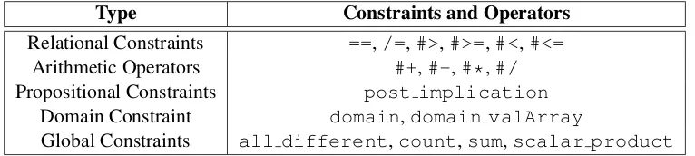
AT OY(F D)programconsists of a set of data constructors and a set of functions, that can be higher-order and non-deterministic (with possibly several reductions for given, even ground, arguments). The syntax is mostly borrowed from Haskell [PJ02], with the remarkable excep-tion that program and type variables begin with upper-case letters whereas data constructors, types and functions begin with lower-case. The repertoire ofF D constraints and operators is presented in Table1, also including ==and/=, as they are truly polymorphic (with the same operators forH andF D).
Type Constraints and Operators
Relational Constraints ==,/=,#>,#>=,#<,#<= Arithmetic Operators #+,#-,#*,#/ Propositional Constraints post implication
Domain Constraint domain,domain valArray
Global Constraints all different,count,sum,scalar product
Table 1: Repertoire ofF DConstraints and Operators
patterndenotes a data value not subject of further evaluation (this includes variables, constants, data constructors and partial application of functions). A (user-)defined functionis character-ized by an optional principal type, which is checked/inferred by the system, and by a set of constrained rewriting rules f t1. . .tn =e ⇐= l1==r1, . . . ,lk==rk wheret1, . . . ,tn form a tu-ple of linear patterns (i.e., with no repeated variables), ande,li,ri are expressions. Rules have a conditional reading: f t1. . .tncan be reduced toeif all the constraintsl1==r1, . . . ,lk ==rk are satisfied. For the case of non-deterministic functions, rules are applied following their tex-tual order, and both failure and user request for a new solution trigger backtracking to the next unexplored rule.
AT OY(F D)goalconsists of a set of constraints. Goal solving follows lazy narrowing: If a constraint is either an equality/disequality Herbrand constraint between patterns or a primitive finite domain constraint, then it is directly posted to its corresponding solver. Otherwise, the arguments of the constraint being expressions are lazily evaluated, applying matching function rules. This transforms the initial constraint into a primitive one, possibly producing more prim-itive or composed constraints to be processed. Once all the constraints of the goal have been processed, aT OY(F D)solutionconsists of the simplifiedH andF Dconstraint stores.
3
Search Primitives
This section presents eight newT OY(F D)primitives for specifying search strategies, allow-ing the user to interact with the solver in the search for solutions. Each primitive is presented from an abstract (solver independent) point of view, emphasizing some novel search concepts they provide. The specification of some search criteria atT OY(F D)level and the combina-tion of primitives (to specify complex search strategies) are also presented.
3.1 Labeling Primitives
In this section, four search primitives are described:lab,labB,labWandlabO.
Primitive lab
lab :: varOrd -> valOrd -> int -> [int] -> bool
myVarOrder:: [int] -> int
myVarOrder V = fst (foldl cmp (0,0)
(zip (take (length V) (from 0)) (map (length . get_dom) V))) %
myValOrder:: [[int]] -> int | from:: int -> [int]
myValOrder D = head (last D) | from N = [N | from (N+1)]
%
cmp:: (int,int) -> (int,int) -> (int,int)
cmp (I1,V1) (I2,V2) = if (V1 >= V2) then (I1,V1) else (I2,V2) ---TOY(FD)> domain [X,Y,Z] 0 4, Y /= 1, Y /= 3, Z /= 2,
lab userVar userVal 2 [X,Y,Z], ... (rest of goal)
Figure 1: Variable and Value User-Defined Criteria
To express them we have defined inT OY the enumerated datatypesvarOrd andvalOrd, covering all the predefined criteria available in the Gecode documentation [STL13]. They also include a last case (userVaranduserVal, respectively) in which the user implements its own variable/value selection criteria atT OY(F D)level. The third elementNrepresents how many variables of the variable set are to be labeled. This represents a novel concept which is not available in the predefined search strategies of Gecode and ILOG Solver. The fourth argument represents the variable setS. Thus, the search heuristic usesvarOrdto label justNvariables of S.
Figure1presents aT OY(F D)program (top) and goal (bottom) showing how expressive, easy and flexible is to specify a search criteria inT OY(F D). In the example, the search strat-egy of the goal uses the userVarand userVal selection criteria (specified by the user in the functionsmyVarOrderandmyValOrder, respectively). Thelabsearch strategy is ap-plicable to the constraint network posted by theT OY(F D)goaldomain [X,Y,Z] 0 4, Y /= 1, Y /= 3, Z /= 2. Then, the computation continues by processing the “rest of goal” for each feasible solutions found by the lab strategy. It acts over the set of variables [X,Y,Z], but it is only expected to label two of them.
The function myVarOrder selects first the variable with more intervals in its domain. It receives the list of variables involved in the search strategy, returning the index of the selected one. To this end, it uses the auxiliary functionsfromandcmp; the predefined functionsfst, foldl, zip, take, length, map, head, last and(.) (all of them with an equivalent semantics to those of Haskell); and the reflection functionget dom, which accesses the internal state of the solver to obtain the domain of a variable (this domain is presented as a list of lists, where each sublist represents an interval of values).
The function myValOrderreceives as its unique argument the domain of the variable, re-turning the lower bound of its upper interval. So, in conclusion, the first two solutions ob-tained by the lab strategy are: {X in 0..4, Y -> 4, Z -> 3} and {X in 0..4, Y -> 4, Z -> 4}.
Primitive labB
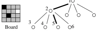
This primitive uses the same four basic elements aslab. However, its behavior is different, as it follows thevarOrdandvalOrdcriteria to explore just one branch of the search tree, with no backtracking allowed. The 4-Queens problem is used to explain this behavior.
Using lab unassignedLeftVar smallestVal 0 [X1,X2,X3,X4] (where 0 in the third argument stands for labeling all the variables) two solutions are obtained: {X1 -> 1, X2 -> 3, X3 -> 2, X4 -> 4} and {X1 -> 2, X2 -> 4, X3 -> 1, X4 -> 3}. However, iflabB unassignedLeftVar smallestVal 0 [X1,X2,X3,X4] is used, then the strategy fails, getting no solutions. Figure2(4×4 square board and tree) shows the compu-tation process. First, the selected criteria assignsX1 -> 1at root node (1), leading to node2. Propagation reduces the search space to{X2 in 3..4, X3 in 2 ∨4, X4 in 2..3}, pruning nodes3and4. Then, computation assignsX2 -> 3(leading to node5), and propaga-tion leads to an empty domain forX3. So, the explored tree path leads to no solutions as well as, therefore, its computation. As it is seen, propagation during search modifies the intended branch to be explored (in the goal example, it explores the branch1-2-5instead of1-2-3).
Primitive labW
labW :: varOrd -> bound -> int -> [int] -> bool
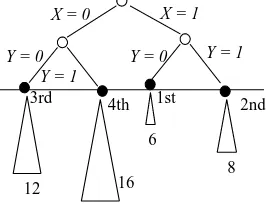
This primitive performs an exhaustive breadth exploration of the search tree, storing the satisfi-able leaf nodes achieved to further sort them by a specified criteria. A first example is considered to understand the behavior oflabW. Figure3presents aT OY(F D)goal with four variables, where two implication constraints relateXandYwithV1andV2, respectively.
Iflab unassignedLeftVar smallestVal 2 [X,Y,V1,V2]strategy had been used (instead of thelabWone) to label the first two unbound vars of[X,Y,V1,V2], then the search would have explored the search tree obtaining (one by one) the next four feasible solutions: {X -> 0, Y -> 0}, {X -> 0, Y -> 1}, {X -> 1, Y -> 0} and {X -> 1, Y -> 1}. Figure4represents the exploration for obtaining those solutions, where each black node represents a solution, and the triangle it has below represents the remaining size of the search space (product of cardinalities ofV1andV2). As it is seen, whereas the first solution computed bylableads to compute the “rest of goal” from a 12 candidates search space, the third solution leads to a 6 candidates one. The primitivelabWexplores exhaustively the search tree in breadth, storing in a data structureDSeach feasible node leading to a solution. Once the tree has been completely explored, the solutions are obtained (one by one) by using a criteria to select and remove thebestnode fromDS. In the example, the selected criteriasmallestSearchTree selects first the node with smaller product of cardinalities ofV1andV2(returning first the solu-tion of the 6 candidates). The order in which thelabWstrategy of the goal delivers the solutions
2
3 5 6 1
4 Board
TOY(FD)> domain [X,Y] 0 1, post_implication X (#=) 1 V1 (#>) 1, domain [V1,V2] 0 3, post_implication Y (#=) 0 V2 (#>) 0, labW unassignedLeftVar smallestSearchTree 2 [X,Y,V1,V2], ... (rest of goal)
Figure 3:labWExample
is presented in Figure4.
Coming back to the definition oflabW, the first parameter represents the variable selection criteria (no value selection is necessary, as the search would be exhaustive for all the values of the selected variables). The second parameter represents thebest node selection criteria. To express it in T OY(F D), the enumerated datatypeord has been defined, ranging from the smallest/largest remaining search space of the product cardinalities of the labeling/solver-scope variables. Again, a last case (userBound) allows to specify the bound criteria atT OY(F D)
level. The third parameter sets the breadth level of exhaustive exploration of the tree (represented as a horizontal black line in Figure4). Finally, as usual, the last parameter is the set of variables to be labeled.
Figure5presents aT OY(F D)program (top) and goal (bottom) with a bound criteria spec-ified in the user functionmyBound. Thebestnode procedure selection traverses all the obtained nodes inDS, selecting first the one with minimal bound value. In this context, the user criteria specified inmyBound assigns to each node (minus) the number of its singleton value search variables. Once again, the functionmyBound also relies on auxiliary, predefined and reflec-tion funcreflec-tions. The first two obtained solureflec-tions are{X -> 1, Y -> 1, A -> 0, B -> 0, C -> 0}and{X -> 2,Y -> 1,A in 0..1,B -> 0,C -> 0}, respectively.
In summary,labWrepresents a novel concept which is not available in the predefined search strategies of Gecode and ILOG Solver. However, it must be used carefully, as exploring the tree very deeply can lead to a explosion of feasible nodes, producing memory problems forDS and becoming very inefficient (due to the time spent on exploring the tree and selecting thebest node).
Primitive labO
labO :: optType -> varOrd -> valOrd -> int -> [int] -> bool This primitive performs a standard optimization labeling. The first parameteroptTypecontains the optimization type (minimization/maximization) and the variable to be optimized. The other four parameters are the same as in thelabprimitive.
1st 2nd 3rd 4th
X = 0 X = 1
Y = 0 Y = 0 Y = 1
Y = 1
6
8 12 16
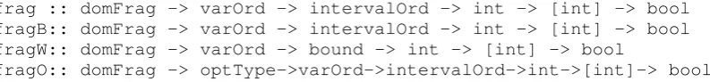
3.2 Fragmentize Primitives
frag :: domFrag -> varOrd -> intervalOrd -> int -> [int] -> bool fragB:: domFrag -> varOrd -> intervalOrd -> int -> [int] -> bool fragW:: domFrag -> varOrd -> bound -> int -> [int] -> bool
fragO:: domFrag -> optType->varOrd->intervalOrd->int->[int]-> bool
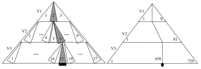
These four new primitives are mate to the labeling ones, but each variable is not labeled (bound) to a value, butfragmented (pruned) to a subset of the values of their domain. An in-troductory example is used to motivate the usefulness of these new primitives: A goal containsV variables andCconstraints, withV’≡ {V1,V2,V3}a subset ofV. The constraintdomain V’ 1 9belongs toC. And no constraint ofCrelates the variables ofV’by themselves, but some constraints relateV’with the rest of variables ofV.
Figure6presents the search tree exploration achieved byfrag*andlab*search primitives, respectively, where search nodes have been numbered. In the case of frag*, the three vari-ables ofV’have been fragmented into the intervals (1,. . .,3), (4,. . .,6) and (7,. . .,9), leading to exponentially less leaf nodes (27) than thelab* exploration (729). On the one hand, if it is known that there is only one solution to the problem, the probabilities of finding the right com-bination ofV’values is thus bigger infrag*than inlab*. On the other hand, the remaining search space of the leaf nodes oflab*are expected to be exponentially smaller than the ones of frag*, due to the more propagation inV’(also expecting to lead to more pruning in the rest of variablesV). Thus, the frag*search strategies can be seen as a more conservative technique, where there are less expectations of highly reducing the search space, as variables are not bound, but there is more probability of choosing a subset containing values leading to solutions (in what can be seen as a sort of generalization offirst-fail). Coming back to the definition of eachfrag* primitive, two main differences arise w.r.t. its matelab*primitive: First, it contains as an extra basic component (first argument) the datatypedomFrag, which specifies the way the selected variable is fragmented. The user can choose betweenpartition nandintervals. The former fragments the domain values of the variable intonsubsets of the same cardinality. The latter looks for already existing intervals on the domain of the variables, splitting the domain on them. For example, in the goaldomain [X] 0 16, X /= 9, X /= 12whereas apply-ingpartition 3toXfragments the domain in the subsetsS1≡ {0. . .4},S2≡ {5. . .8}∪{10}
andS3≡ {11}∪{13. . .16}, applyingintervalsfragments the domain in the subsetsS1’≡ isBound:: [[int]] -> bool
isBound [[A,A]] = true
isBound [[A,B]] = false <== B /= A
isBound [[A,B] | RL] = false <== length RL > 0 %
myBound:: [int] -> int
myBound V = - (length (filter isBound (map get_dom V))) ---TOY(FD)> domain [X,Y] 1 2, domain [A,B,C] 0 5,
A #< X, B #< Y, C #< Y,
labW unassignedLeftVar userBound 2 [X,Y,A,B,C]
… …
V3 1
1 2 3
5 6 9 1 4
16 18 17 27
… …
1 81 1 9
V3 V2
V1
729
1 450
V1
V2
Figure 6:fragvs.labSearch Tree
{0. . .8},S2’ ≡ {10. . .11}andS3’≡ {13. . .16}. As a second difference, it contains an enu-merated datatypeintervalOrd(replacing thelab*argumentvalOrd), to specify the order in which the different intervals should be tried: First left, right, middle or random interval.
In summary, it is claimed thatfrag*primitives are an remarkable tool, to be taken into ac-count in the context of search strategies as an alternative or a complement to the use of exhaustive labelings. Also, its use inT OY(F D)represents a novel concept which is not available in the predefined search strategies of Gecode and ILOG Solver.
3.3 Applying Different Search Scenarios
The use ofT OY(F D)non-deterministic functions allows to sequentially apply different search strategies for solving a problem. For example, after postingVandCto the solver, theT OY(F D)
program (top) and goal (bottom) presented in Figure7uses the non-deterministic functionfto specify three different scenarios for the solving of the goal described in Section3.2. Each sce-nario ends with an exhaustive labeling of the set of variablesV. However, the search spacesthis exhaustive labeling has to explore can be highly reduced by the previous evaluation off.
Scenario 1: The first rule offperforms the search heuristich1overV’≡ {V1,V2,V3}. h1
fragments the domain ofV1into 4 subsets, selecting one randomly. If propagation succeeds, then h1boundsV2andV3to their smallest value. If propagation succeeds (with a remaining search spaces1), thenh1succeeds, and the exhaustive labeling exploress1. If propagation fails in one of
those points, or the exhaustive labeling does not find any solution ins1, thenh1completely fails
f:: [int] -> bool
f [V1,V2,V3] = true <==
fragB (partition 4) unassignedLeftVar random 0 [V1], labB unassignedLeftVar smallestVal 0 [V2,V3]
f [V1,V2,V3] = true <==
fragW (partition 4) unassignedLeftVar smallestTree 0 [V1], labB unassignedLeftVar smallestTotalVars 0 [V2,V3]
f [V1,V2,V3] = true
---TOY(FD)> Post of (V,C), f V’, lab userVar userVal 0 V
(as well as the first rule off), as both thelabBandfragBprimitives just explore one branch. Scenario 2: The second rule offis tried, performing the heuristich2overV’. Here afragW primitive is first applied. So, if further eitherlabBofh2or the exhaustivelab(acting overs2)
fails, backtracking is performed overfragW, providing the nextbestinterval ofV1(according to the smallest search tree criteria, as in Figure4). If, after trying all the intervals a solution is not found, thenh2completely fails (as well as the second rule off).
Scenario 3: If both h1 andh2 fail, the third rule offtrivially succeeds, and the exhaustive
labeling is performed over the original search space obtained after postingVandCto the solver.
4
Implementing the Search Primitives
The implementation of the eight new search primitives is based on the Gecode and ILOG Solver underlying search mechanisms. First, an abstract specification of the requirements the new
T OY(F D)search strategies must fulfill is presented. Then, it is described how to adapt those requirements to Gecode and ILOG Solver.
4.1 Abstract Specification of the Search Strategy
A single entry point (C++ function) for the different primitives is specified. Its proposed al-gorithm is parameterizable by the primitive type and its basic components. It is described as follows:
1. The algorithm explores the tree by iteratively selecting a variablevarand a valuev, cre-ating two options: (a) Postvar == v. (b) Postvar /= vto continue the exploration taking advantage of the previously explored branch, recursively selecting another value to perform again (a) and (b).
2. Forfrag* strategies it selects an intervaliinstead of a value, posting in (a) bothvar #>= i.min and var #<= i.max. However, the (b) branch can not take advantage by postingvar #< i.minandvar #> i.max, as the constraint store would become inconsistent. Thus, (b) just removesifrom the set of intervals, and continue the search by selecting a new interval.
3. ForlabBandfragBstrategies, only the (a) option is tried.
4. ForlabO andfragOstrategies, branch and bound techniques are used to optimize the search.
5. Specific functions are devoted to variable and value/interval selection strategies, as well as to the bound associated to a particular solution found by labW and fragW. Those functions include the possibility of accessing Prolog, to follow the criteria the user has specified atT OY(F D)level (usingT OY(F D)functions which are compiled to mate Prolog predicates).
on demand. Thus,sscontains an entity performing the search and a vectorDS(cf. Sec-tion 3.2) containing the solutions. The notion of solution is abstracted as the necessary information to perform the synchronization fromssto the main constraint solver. Also, a status indicates whether the exploration has finished or not.
7. The algorithm finishes (successfully) as it founds a solution, except forlabWandfragW strategies, where it stores the solution node and triggers an explicit failure, continuing the breadth exploration of the tree.
8. A counter is used to control that only the specified amount of variables of the variable set is labeled/pruned.
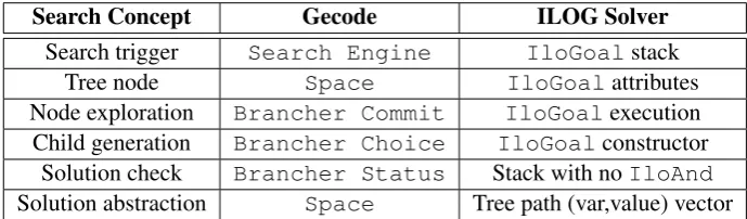
Next two sections adapt this specification to Gecode and ILOG Solver, respectively. Table2 summarizes the different notions provided by both libraries.
4.2 Gecode
Search strategies in Gecode are specified viaBranchers, which are applied to the constraint solver (Space) to define the shape of the search tree to be explored. TheSpaceis then passed to aSearch Engine, whose execution method looks for a solution by performing a depth-first search exploration of the tree. This exploration is based on cloningSpaces(twoSpaces are said to be equivalent if they contain equivalent stores) and hybrid recomputation techniques to optimize the backtracking. As Spaces constitute the nodes of the search tree, a solution found by theSearch Engineis a new Space. The library allows to create a new class of Brancherby defining three class methods: status, which specifies if the current node is a solution, or their children must be generated to continue with their exploration;choice, which generates an objectocontaining the number of children the node has, as well as all the necessary information to perform their exploration;commit, which receivesoand the concrete children identifier to perform its exploration (generating a newSpaceto be placed at that node).
Adaptation to the Specification.The search strategies are implemented via two layers. First, a new class ofBrancher MyGenerate, which carries out the tree exploration by the combi-nation of thestatus,choiceandcommitmethods. As each node of the tree is aSpace, the methods are applied to it. Second, aSearch Engine, controlling the search by receiving the
Search Concept Gecode ILOG Solver
Search trigger Search Engine IloGoalstack
Tree node Space IloGoalattributes
Node exploration Brancher Commit IloGoalexecution Child generation Brancher Choice IloGoalconstructor
Solution check Brancher Status Stack with noIloAnd Solution abstraction Space Tree path (var,value) vector
initialSpaceand making the necessary clones to traverse the tree. In this setting, the abstract description presented before is instantiated to Gecode as follows:
1. Thechoicemethod deals with the selection of the variablevarand the valuev, creating an objectowith them as parameters, as well as the notion of having two children. The variable selection must rely on an external register r, being controlled by the Search Engine and thus independent on the concrete node (Space) the choice method is working with. The register is necessary to ensure that, whether a father generates its right hand child by postingvar /= v, this child will reuserto select againvar(as a difference to the left hand child, which removes thercontent to select a new variable).
2. Forfrag*strategies, instead of passingvaltoo, thechoicemethod generates a vector with all the different intervals to be tried, and the size of this vector is passed as its number of children.
3. ForlabBandfragB, only one child is considered.
4. For labOandfragO, a specialized branch and boundSearch Engineprovided by Gecode is used.
6 The search entity is theSearch Engineand the solution is aSpace.
7 For labWandfragW, the Search Engineuses a loop, requesting solutions one by one until no more are found (the breadth exploration of the search tree has finished).
8 Only the left hand child oflab*strategies increments the counter value, and thestatus method checks the counter to stop the search at the precise moment.
4.3 ILOG Solver
Search strategies in ILOG Solver are performed via the execution ofIloGoals. AnIloGoal is a daemon characterized by its constructor and its execution method. The constructor creates the goal, initializing its attributes. The execution method triggers the algorithm to be processed by the constraint solver (IloSolver), and can include more calls to goal constructors, making the algorithm processed byIloSolverto be the consequence of executing severalIloGoals. AnIloGoalfails ifIloSolverbecomes inconsistent by running its execution method; oth-erwise the goal succeeds. The library allows to create a new class ofIloGoalby defining its constructor and execution method. Four basic goal classes are provided for developing new goals with complex functionality. GoalsIlcGoalTrueandIlcGoalFalsemake the current goal succeed and fail, respectively. GoalsIlcAndandIlcOr, both taking two subgoals as argu-ments, make the current goal succeed depending on the behavior of its subgoals. WhileIlcAnd succeeds only if its two subgoals succeed,IlcOrcreates a restorable choice point which exe-cutes its first subgoal, restores the solver state at the choice point on demand, and exeexe-cutes its second subgoal.
variable, the latter deals with its binding/prunning to a value/interval. In this setting, the abstract description presented before is instantiated to ILOG Solver as follows:
1. The control of the tree exploration is carried out byMyGenerate, which selects a vari-able and uses the recursive callIlcAnd(MyInstantiate, MyGenerate)to bind it and further continue processing a new variable. InMyInstantiate, the alternatives (a) and (b) are implemented with IlcOr(var == val, IlcAnd( var /= var, MyInstantiate)).
2. It dynamically generates a vector with the available intervals on each differentMyGenerate call.
3. Only the goalvar == valis tried.
4. The branch and bound is explicitly implemented. Thus, before selecting each new vari-able, it is checked if the current optimization variable can improve the bound previously obtained; otherwise anIloGoalFailis used to trigger backtracking (as well as if, af-ter labeling the required variables, the obtained solution does not bind the optimization variable).
6 The entity performing the search is anIloSolver. Also, a solution is represented by a vector of integers (representing the indexes of the labeled/pruned variables) and a vector of pairs, representing the assigned value or bounds of these variables. This explicit solution entity is built towards the recursive calls ofMyGenerate, which adds on each call the index of the variable being labeled. Once found the solution, it stores it inDS.
7 After storing a solution inlabWorfragW, anIloGoalFalseis used, triggering back-tracking to continue the breadth exploration.
8 Each call toMyGenerateincrements the counter value.
5
Performance
This section analyzes the new performance achieved byT OY(F Dg)andT OY(F Di). The benchmark includes four of the CP(F D) problems available at CSPLib [HMGW]: Magic Se-quence,N-Queens,Langford’s numberandGolomb Rulers. The set of problems is claimed to be representative enough because: First, all are parametric, and thus they allow to test the perfor-mance of theT OY(F D)versions as the instances of each problem scale. And, second, they include the whole set ofF Dconstraints of theT OY(F D)repertoire.
The structure of the solutions of each problem is discussed, pointing out how the new search strategies reduce the search exploration to find them. Thus, for each problem, twoT OY(F D)
models are created: problem bs.toy, which applies a singlelabelingprimitive as its search strategy; problem is.toy, which applies some of the new proposed search primitives before ap-plying the endinglabeling(to still guarantee completeness of the search process).
T OY(F Dg)C++ code. All theT OY(F D)models are available at:http://gpd.sip. ucm.es/ncasti/models.zip. For the sake of simplicity, from now on the different ver-sions of the models will be simply referred to asbsandis.
5.1 Analyzing the Applied Search Strategies
Magic Sequence.Thebsmodel uses a singlelabeling [ff] Las its search strategy. Ana-lyzing the solutions of the problem it is observed that, if the parametern≥9 then the sequence follows the pattern: L≡[(n−4),2,1,0,0, . . . ,1,0,0,0]. In this context, the new search strat-egy of theismodel first applieslabB unassignedRightVar smallestVal 3 L, labB unassignedRightVar largestVal 1 L, which matches the last four variable 1,0,0,0 pattern. At that point, propagation leads toL≡[(n−4),A,B,C,0, . . . ,1,0,0,0](withAin 1..3,B in 0..1 andCin 0..1), highly reducing the search space the furtherlabelinghas to deal with.
Queens. Thebsmodel uses a singlelabeling [ff] Las its search strategy. Analyzing the solutions of the problem, an intuitive way for reducing the initial search space of the problem consists of: First, splitting thenvariables intokvariable sets(vs1,vs2, . . . ,vsk)(where consecu-tive variables are placed in different variable sets). Second, splitting the initial domain 1. . .ninto kdifferent intervals(1..(n/k), . . . ,(n/k)∗(i−1) +1..(n/k)∗i, . . . ,(n/k)∗(k−1) +1..n). And, finally, assigning the variables ofvsito theithinterval.
In this context, the new search strategy of theismodel first appliessplit into 3 L ([], [], []) == (K1,K2,K3), fragB (partition 3) unassignedLeftVar
firstRight 0 K1, fragB (partition 3) unassignedLeftVar firstMiddle 0 K2, fragB (partition 3) unassignedLeftVar firstLeft 0 K3. This splits the variables and their domains into three sets, highly reducing the search space the further labelinghas to deal with.
Langford’s Number. The bsmodel uses a single labeling [ff] Las its search strat-egy. Analyzing the solutions of the instances proposed, it is observed that they follow the pat-tern: L≡[X1,X2, . . . ,A,B,C,D,E,F], with an inductive mapping between the set of variables
{A,B,E,F}and the set of values{1,2,3,4}. In this context, the new search strategy of the is model first appliesfragB (partition ((round ((M*N)/4)) - 1)) unassigned-RightVar firstLeft 0 [A,B,E,F], labW unassigned- unassigned-RightVar smallest-TotalDomain 0 [A,B,E,F].
Golomb Rulers. The bs model uses a single labeling [toMinimize Mn] M as its search strategy. Analyzing the solutions of the instances proposed, it is observed that the ini-tial domain of their variables is huge, and that the value they take in the optimal solution is not far away from their initial lower bound. For example, in G-11 (an instance benchmark for 11 rulers, for whichM≡[0,A,B, ...,H,I,J]), the initial domains of the last three variables areHin 36..1020,I in 45..1021 andJ in 55..1023 (with known optimal solution 64, 70 and 72, respec-tively) and the initial domain of the first three variables is 0,Ain 1..977 andBin 3..987 (with known optimal solution 0, 1 and 4, respectively).
In this context, an intuitive way of reducing the initial search space is by reducing as much as possible the upper bound of these variables. The new search strategy of theismodel first applies
fragW (partition 3) unassignedRightVar smallestSearchTree 2 L,fragW
(partition 12) unassignedLeftVar largestSearchTree 2 L, fragmenting first the last two variables and then the first two. Note that, whereas the former selects asbest interme-diate node the one minimizing the remaining search space, the latter selects the one maximizing it (which intuitively makes sense, as the smaller interval is the one pruning the least the upper bound of the first two variables, thus pruning less the search space).
5.2 Running the Experiments
Table3compares the performance of matebsandisinstances. Columns 2 and 4 represent the CPU solving time in seconds ofbsandis(respectively), both of them using incremental prop-agation mode. Columns 3 and 5 represent the speed-up ofT OY(F Dg)w.r.t. T OY(F Di)
forbsandis, respectively. Finally, column 6 focuses on each concrete T OY(F D) version, representing the speed-up ofisw.r.t.bs. Some conclusions are obtained:
First, the use of the new search strategies is encouraging, as the performance ofT OY(F Dg)
andT OY(F Di)for solvingisinstances is better than the achieved for solvingbsones (except-ing Q-90 and L-119, whereT OY(F Di)spends about 0.4 seconds more in solvingis). In any case, the differences range from a 5% to nearly the 100%, so a more detailed analysis by prob-lems and instances is required.
For Queens and Langford’sisinstances, the better performance achieved by T OY(F Dg)
andT OY(F Di)clearly scales as the sizes of the instances scale. More specifically, for Q-90 and L-119 (solved in tenths of seconds)T OY(F Dg) achieves an improvement of 22% and 5%, respectively. This improvement grows an order of magnitude for Q-105 and L-127 (with an improvement of 92%) and two orders of magnitude for Q-120 and L-131 (with an improvement of nearly the 100%). InT OY(F Di), it is observed the same growing pattern, but it is less noticeable. For Q-90 and L-119 the isperformance is even worse than the bsone. Then, for Q-105 and L-127 theisperformance improves a 38% and a 63%, respectively, but still in the same order of magnitude asbs. Finally, for Q-120 and L-131 theisperformance reaches the two orders of magnitude improvement w.r.t.bs, reaching nearly a 100%.
For Magicisinstances, the better performance achieved byT OY(F Dg)andT OY(F Di)
remains stable as the size of the instances scale (with around a 33%-34% forT OY(F Dg)and a 23%-24% forT OY(F Di)). Last, for Golombisinstances the better performance decreases a 20% per instance (as they scale), with a 75%, 60% and 41% improvement ofT OY(F Dg)
Instance bs Sp-Up is Sp-Up on/off
M-400 FDi 0.530 1.00 0.402 1.00 0.76 M-400 FDg 0.422 0.80 0.280 0.70 0.66
M-900 FDi 2.53 1.00 1.95 1.00 0.77
M-900 FDg 2.00 0.79 1.34 0.69 0.67
Q-90 FDi 0.110 1.00 0.514 1.00 4.67 Q-90 FDg 0.078 0.71 0.061 0.12 0.78
Q-105 FDi 1.25 1.00 0.78 1.00 0.62
Q-105 FDg 1.05 0.84 0.08 0.10 0.08
Q-120 FDi 154.00 1.00 1.11 1.00 0.01 Q-120 FDg 129.88 0.84 0.09 0.08 0.00 L-119 FDi 0.530 1.00 0.984 1.00 1.86 L-119 FDg 0.296 0.56 0.282 0.29 0.95
L-127 FDi 4.35 1.00 1.17 1.00 0.27
L-127 FDg 4.62 1.06 0.39 0.33 0.08
L-131 FDi 87.00 1.00 1.19 1.00 0.01 L-131 FDg 98.53 1.13 0.33 0.28 0.00
G-9 FDi 0.421 1.00 0.109 1.00 0.26 G-9 FDg 0.250 0.59 0.062 0.57 0.25
G-10 FDi 3.56 1.00 1.47 1.00 0.41
G-10 FDg 2.11 0.59 0.84 0.57 0.40
G-11 FDi 72.65 1.00 43.98 1.00 0.61 G-11 FDg 42.01 0.58 24.85 0.57 0.59
Table 3: Performance ofT OY(F D)using the Search Strategies
Second, it is clearly observed that the improvement achieved byT OY(F Dg)forisinstances is bigger than the one achieved byT OY(F Di), revealing that the approach Gecode offers to extend the library with new search strategies is more efficient than the one of ILOG Solver. That is, for any isinstance, the speed-up of T OY(F Dg) w.r.t. T OY(F Di) is bigger than the achieved for its matebsinstance.
In this context, two different behaviors are observed. First, for Queens and Langford’s is instances the speed-up improvement achieved w.r.t.bsinstances increases as the instances scale: A 59%, 74% and 76% for Q-90, Q-105 and Q-120, respectively. A 27%, 73% and 85% for L-119, L-127 and L-131, respectively. Second, for Magic and Golombisinstances the speed-up improvement achieved w.r.t.bsinstances remains stable as the instances scale: A 10% for M-400 and M-900. A 2%, 2% and 1% for G-9, G-10 and G-11, respectively.
6
Related Work
[STW+13]. It provides a lightweight and solver-independent method bridging the gap between a conceptually simple search language (high level, functional and naturally compositional) and an efficient implementation (low-level, imperative and highly non-modular). T OY(F D) is more rigid than [STW+13], but some of the features provided by the search combinators can be matched with the new set of primitives presented in Section3: The basic primitive heuris-tics base search andprune can be obtained with the primitive lab, controlling the ex-act number of variables to be labeled (which allowsT OY(F D)to support composite search strategies). Regarding the set of combinators proposed,T OY(F D)matches{let,assign, post}via intermixing search procedures with constraint posting, and{and,or}via the com-posed search strategies presented in Section3.3. Finally, theT OY(F D) primitives are also extensible, as users can program their own criteria atT OY(F D)level with no extra effort at the SICStus and C++ core implementation of the system.
Similar approaches to search combinators are proposed for Constraint Funcional Programming (CFP(F D)), with Monadic Constraint Programming [SSW09], and for CLP(F D), with the library Tor [STD12] (available in SWI-Prolog). They decouple the definition of the search tree and the search method. In T OY(F D), it is not possible to specify the way to explore the search tree (as, for example, by limited discrepancy search). However, the primitiveslabWand fragWperform a breadth search exploration. Also, whereas these primitives include a depth bound, it can be implicitly imposed as well for the rest of primitives (by using the parameter setting the amount of variables to be labeled). Moreover, at least inT OY(F Dg)it would not be difficult to support new ways of exploring the search tree, as the Gecode library provide the mechanisms to implement them.
7
Conclusions and Future Work
This paper has presented eight newT OY(F D) search primitives, describing their behavior from a solver independent point of view, and using examples to show their application. It has emphasized the novel concepts those primitives include, as performing an exhaustive breadth exploration of the search tree further sorting the satisfiable solutions by a specified criteria, frag-menting the domains of the variables by pruning each one to a subset of its domain values instead of binding it to a single value, and applying the labeling or fragment strategy only to a subset of the variables involved. It has also pointed out how expressive, easy and flexible it is to specify some search criteria atT OY(F D)level, and also to apply different search strategies (setting different search scenarios) to the solving of a CP(F D) problem.
A new version ofT OY(F Dg)andT OY(F Di)including these search primitives has been presented. It has been described their implementation in Gecode and ILOG Solver, by extending their libraries relying on their underlying search mechanisms. It has been observed that these search mechanisms are quite different in Gecode (Search Engine, Brancher methods, hybrid recomputation) and ILOG Solver (IloGoal, goal constructor, goal stack). Thus, an abstract view of the requirements needed to integrate the search strategies inT OY(F D)has been first presented (with the scheme further instantiated to Gecode and ILOG Solver).
ei-ther with a classicallabelingand with an improvedad hocsearch strategy have been devel-oped. It has been proven that the use of the new search strategies improve the performance of both T OY(F Dg) andT OY(F Di), but the improvement achieved (ranging in 5%-100%) is dependent on the concrete problem and instance solved: Whereas for Queens and Langford’s instances the better performance achieved clearly scales as the sizes of the instances scale, for Magic ones it remains stable, and for Golomb ones it decreases. Moreover, the speed-up of
T OY(F Dg) w.r.t. T OY(F Di) is bigger for the new improvedT OY(F D) models, re-vealing that the approach Gecode offers to extend the library with new search strategies is more efficient than the one of ILOG Solver.
As future work, we will analyze the applicability of the search strategies presented in this paper to other CP(F D) paradigms. In particular, we will implement the search primitives in the CFP(F D) system Monadic Constraint Programming, the CLP(F D) system Tor and the C++ CP(F D) system Gecode (using the search combinators [STW+13] to implement the strategies). We will discuss if there are aspects ofT OY(F D)that are not easily implemented in the other systems, such as the use of non-deterministic functions (to apply different search scenarios to tackle a problem), and the specification of some search criteria in the proper native language (and the impact it may have in the system architecture). We will also reuse the benchmark used in this paper to compare the solving efficiency achieved by each system when applying thead hocstrategies, analyzing any possible overhead arisen due to their use.
Besides that, focusing again in T OY(F D), scripting techniques can be applied, to solve the benchmarks under multiple and very precisely controlled scenarios. In them, an exhaustive combination of applying one or different search strategies (as well as the variable subset used on each of them) will be studied. The results will be analyzed, in order to find out which strategies had lead to a solution or, at least, to a minimum search space containing a solution. Moreover, this analysis will help to find out new patterns about the relation between the structure of a concrete problem and the concrete search strategy (or combination of search strategies) to be applied to successfully solve it.
Bibliography
[CS12] I. Casti˜neiras, F. S´aenz-P´erez. Improving the Performance of FD Constraint Solving in a CFLP System. InFLOPS’12, 88–103. LNCS 7294. Springer, 2012.
[FHSV07] A. J. Fern´andez, T. Hortal´a-Gonz´alez, F. S´aenz-P´erez, R. del Vado-V´ırseda. Con-straint Functional Logic Programming over Finite Domains.TPLP7(5):537 – 582, 2007.
[Gec] Gecode: Generic Constraint Development Environment. Version 3.7.3.http://www. gecode.org/.
[Han07] M. Hanus. Multi-Paradigm Declarative Languages. InICLP’07, 45–75. LNCS 4670. Springer, 2007.
[HMGW] B. Hnich, I. Miguel, I. P. Gent, T. Walsh. CSPLib: A Problem Library for Con-straints.http://www.csplib.org/.
[ILO10] IBM ILOG CP 1.6. 2010.http://www-947.ibm.com/support/entry/portal/Overview/ Software/WebSphere/IBM ILOG CP.
[JM94] J. Jaffar, M. Maher. Constraint Logic Programming: A Survey. In The Journal of Logic Programming, 19–20. 503–581. Elsevier, 1994.
[LLR93] R. Loogen, F. L´opez-Fraguas, M. Rodr´ıguez-Artalejo. A Demand Driven Computa-tion Strategy for Lazy Narrowing. InPLILP’93, 184–200. LNCS 714, 1993.
[LRV04] F. L´opez-Fraguas, M. Rodr´ıguez-Artalejo, R. Vado-V´ırseda. A Lazy Narrowing Cal-culus for Declarative Constraint Programming. InPPDP’04, 43–54. ACM, 2004.
[MS98] K. Marriot, P. J. Stuckey.Programming with Constraints. MIT Press, 1998.
[PJ02] S. Peyton-Jones. Haskell 98 Language and Libraries: the Revised Report. Technical report, 2002.http://www.haskell.org/onlinereport/.
[SIC] SICStus Prolog.http://www.sics.se/.
[SSW09] T. Schrijvers, P. Stuckey, P. Wadler. Monadic Constraint Programming.Journal of Functional Programming19(6):663–697, 2009.
[STD12] T. Schrijvers, M. Triska, B. Demoen. Tor: Extensible Search with Hookable Dis-junction. InPPDP’12, 103–114. ACM, 2012.
[STL13] C. Schulte, G. Tack, M. Z. Lagerkvist. Modeling and Programming with Gecode. 2013.http://www.gecode.org/doc-latest/MPG.pdf.
[STW+13] T. Schrijvers, G. Tack, P. Wuille, H. Samulowitz, P. Stuckey. Search combinators. Constraints18(2):269–305, 2013.