Engineering Problems Solving BY Analytical Mathematical Approach

*Correspondence to Author:

Gangadharaiah, Y. H

Department of Mathematics, Sir M. Visvesvaraya Institute of Technolo-gy,Bangalore-562157, India

How to cite this article:

Gangadharaiah, Y. H, Engineering Problems Solving BY Analytical Mathematical Approach. American Journal of Computer Sciences and Applications, 2017; 1:4.

eSciPub LLC, Houston, TX USA. Website: http://escipub.com/

American Journal of Computer Sciences and Applications

(ISS

N

:2

5

7

5-

77

5X

)

Research Article AJCSA, 2017, 1:

Engineering Problems Solving BY Analytical Mathematical

Approach

Learning how to approach and solve problems which relate to real world situations is an integral part of the education of many higher and further education students and is particularly relevant to students studying for a professional degree. Mathematics is widely used in every engineering fields. In this paper, several examples of applications of mathematics in, civil, chemical and electrical engineering are discussed. Applications here are the

real ones found in the engineering fields, which may not be the

same as discussed in many mathematics text books. Methodolo-gies used are of general interest and may be applicable in other, unrelated, disciplines.

Keywords: Civil; Euler Column; Chemical: Transmission Line.

Gangadharaiah, Y. H

Department of Mathematics, Sir M. Visvesvaraya Institute of Technology,Bangalore-562157, India

1.Introduction

Education of professionally oriented students normally includes three quite different and distinct components which must be integrated in any suitable program of studies. These components comprise the acquisition and understanding of fundamental knowledge, the application of this knowledge to practical, as opposed to theoretical, problems, and the development of skills which are required for professional practice. The first and last of these components pose few difficulties. Acquisition of knowledge is generally handled by the use of lectures, tutorials and seminars while skills are developed during periods of practical work spread over the duration of the academic program. Application of fundamental knowledge to real world problems does, however, cause considerable difficulty largely because real problems can be solved in an infinite variety of different ways and because considerable creativity is necessary to develop the optimum solution. For many years professional schools concentrated primarily on the transfer of knowledge and largely ignored application and skills.

Mathematical modeling has always been an important activity in science and engineering. The formulation of qualitative questions about an observed phenomenon as mathematical problems was the motivation for and an integral part of the development of mathematics from the very beginning. Although problem solving has been practiced for a very long time, the use

of mathematics as a very effective tool in problem solving has gained prominence in the last 50 years, mainly due to rapid developments in computing. Computational power is particularly important in modeling engineering systems, as the physical laws governing these processes are complex. Besides heat, mass, and momentum transfer, these processes may also include chemical reactions, reaction heat, adsorption, desorption, phase transition, multiphase flow, etc. This makes modeling challenging but also necessary to understand complex interactions. All models are abstractions of real systems and processes. Nevertheless, they serve as tools for engineers and scientists to develop an understanding of important systems and processes using mathematical equations. In all engineering context, mathematical modeling is a prerequisite for: design and scale-up; process control; optimization; mechanistic understanding; evaluation/planning of experiments; trouble shooting and diagnostics; determining quantities that cannot be measured directly; simulation instead of costly experiments in the development lab; feasibility studies to determine potential before building prototype equipment or devices.

is now. Linear algebra, calculus, statistics, differential equations and numerical analysis are taught as they are important to understand many engineering subjects such as fluid mechanics, heat transfer, electric circuits and mechanics of materials to name a few. However, there are many complaints from the students who find it difficult to relate mathematics to engineering. After studying differential equations, they are expected to be able to apply them to solve problems in heat transfer, for example. However, the truth is different. For many students, applying mathematics to engineering problems seems to be very difficult. Many examples of engineering applications provided in mathematics textbooks are often too simple and have assumptions that are not realistic. See([8],[9],[10],[11] [15],[16],[17],[18]) for a good textbook which discusses mathematical modelling with real life applications. A lot of problems solved using Maple and MATLAB are given in [12,13,14,]. The purpose of this paper is to show some applications of mathematics to various engineering fields. The applications discussed do not need advanced mathematics so they can be understood easily.

2.

Mathematical

Approach

to

Engineering Problems

In this section we discussed four engineering problems, first problem is about civil circuit problem, the second on the chemical mixing and the last on shape of a transmission line problem .

2. 1. Civil engineering problem

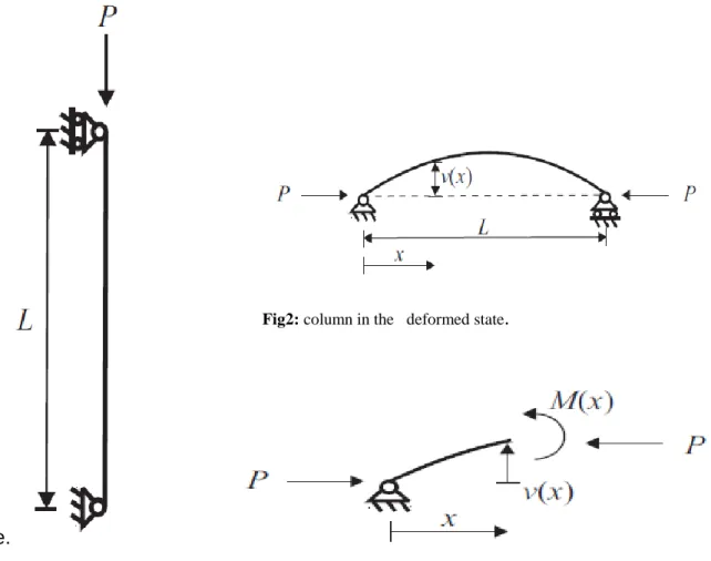
The Euler Column: In Structural Engineering, columns are structural members that are sensitive to buckling, when compressive axial loads are applied, see Figure 1. A column is actually a beam loaded with a compressive force. The so-called buckling load gives the load bearing capacity for relatively slender columns where buckling occurs before yielding (material failure). For buckling analysis, a so-called second order theory is applied in the deformed.

An initial straight beam with length, L , is loaded with a compressive axial force, P, see Figure 1.The beam is simply supported, thus boundary conditions are specified so that it is fixed in one end but allowed to deform axially in the other end. In both ends it is allowed to rotate (the symbols in Figure 1 define this). The buckling load is obtained by analyzing if a state of equilibrium can exist in a deformed state. The transverse deformation at position x is

denoted V x

 

beam (column) into two, adding the so-called section forces and stating that one of the two parts of the beam should be in equilibrium, moment equilibrium gives

 

 

M x  P V x (1)

state.

derivative of the transverse displacement, v:

 

 

 



 



2

, d

M x EI x x V x

dx

 

  (2)

By combining the relations above, the following ordinary linear second order homogeneous differential equation is obtained (the constant _2 is selected in order to ensure a positive coefficient):

 

_{ }

2

2

2 0

d x

x dx



 

  (3)

with boundary conditions 

 

 

Where 2 P

EI

 

The above differential equation suggests an eigenvalue problem and it can be solved directly, we get

 

 

 

     (4)

Applying boundary conditions we get

 

 

0 0 0

0 sin 0 0

B

L A L A







  

    

sin L 0 n , n 1, 2,3... L



    

2 2

2 , 1, 2, 3...

n

n EI

P n

L 

  

Applying boundary conditions we get

 

n

n

x A x

L





  (5)

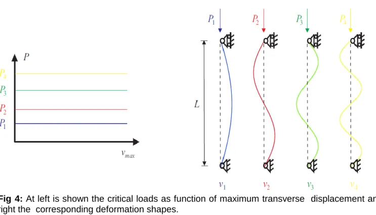
The Pn are so-called critical loads where a state

of equilibrium can exist in the deformed state found before. It can be observed that only the

Fig 1: static model.

Fig2: column in the deformed state.

form of n

 

constant A can not be determined, see Figure 4. Thus, the deformation can be arbitrary large and the column will buckle in practice.

In reality the column will buckle when P1 is reached, which is termed the Euler critical load given by:

2 1 2

e

EI

P P

L 

  (6)

When the load is applied gradually, the column will remain straight until the Euler load, P_e, is

reached and the column will buckle (fail) and the deformation becomes infinite. Higher critical loads can be of practical relevance by constraining the transverse deformation of the column. E.g. if the column is supported in the

transverse direction at the middle,

2 L

x , it will

buckle for the load P₂. In reality a column is not perfect straight and for many practical applications a transverse load is applied, e.g. wind loading on the facade of a building. In these cases it turns out that equilibrium is governed by an inhomogeneous linear second order differential equation.

To summarize, equilibrium of a beam/column loaded in axial compression is governed by an ordinary homogeneous second order differential equation. The solution in terms of eigenvalues and eigen functions is an infinite number of buckling loads and corresponding deformed shapes. In the case of a simply

supported column, only the lowest buckling load is of practical relevance.

2.2. Chemical Engineering

A firm wishes to market bags of lawn fertilizer which contain 25% Nitrogen, 7% Sulfur , and 8% Ammonium. The firm has four chemical precursors C1, C2,C3,C4 which are to be

combined to make the fertilizer. The percentage of each ingredient in a pound of these chemicals is given in Table 1. How much of each chemical should be mixed to obtain 100 pounds of fertilizer meeting

these criteria? Let xi be the number of pounds of chemical Ci used. Then since the total adds up to 100 pounds we have

1 2 3 4 100

x x x x  (7)

Now x₁ pounds of chemical C1 contains

0.20 x₁ pounds of nitrogen, x₂ pounds of C2

contains 0.25 x2 pounds of nitrogen, x3

pounds of C3 contains 0x3 pounds of nitrogen,

and x4 pounds of C4 contains 0.30x4 pounds of nitrogen. Since there should be 0.25 · 100 = 25 pounds of nitrogen in the mixture we obtain

1 2 3 4

0.20x 0.25x 0x 0.30x 25. (8)

Similar expressions can be derived for sulfur and ammonium

1 2 3 4

0.12x 0.05x 0.06x 0.07x 7. (9)

1 2 3 4

0x 0.05x 0.15x 0.1x 8. (10)

1 2 3 4

Fig 4: At left is shown the critical loads as function of maximum transverse displacement and at right the corresponding deformation shapes.

Table 1: Percentage of chemicals

put all together a system of linear equations with augmented matrix

Let





1 1 1 1 : 100

0.2 0.25 0 0.3 : 25 :

0.12 0.05 0.06 0.06 : 7

0 0.05 0.15 0.1 : 8 A B

 

 

 



 

 

 

Using Gaussian elimination, we get

1 0 0 0 : 11.74

0 1 0 0 : 25.08

0 0 1 0 : 8.75

0 0 0 1 : 54.60

 

 

 

 

 

 

1 11.74, 2 25.08, 3 8.75 & 4 54.60.

x  x  x  x 

2.3. Shape of transmission lines

The problem we want to deal with: What is the shape of a transmission line?

To make things simple we assume that a transmission line acts as a homogeneous flexible inextensible string hanging from two points only under the influence of gravity.

 





1 1 ˆ ˆ

S k i f x j



   (12)

1

C C2 C3 C4

Nitrogen 20 25 0 3

Sulfur 12 5 6 7

Fig.1: String forces and gravity acting on a part of the string









2 2 ˆ ˆ

S k i f x h j



   (13)





T  s gk



   (14)

is the density per unit length

g is the gravity acceleration

Note that the string forces acts in direction of the curve tangents.

Projection on the x-axis give

1 2 0 1 2

k k k k k

      for all x

and projection on the y-axis gives

 





1 1

k f x k f x h g S

     (15)

 





1 1

f x f x h g S

h k h



   _ 

(16)

Letting h0in the last equation leads to

 

11 1

,

ds k

f x a

a dx g

  (17)

where ds is the arch length element.

Substituting 1 f1

 

 

 

11 1 1

1

f x f x

a

  a second order

differential equation. By setting u x

 

 

second order equation can be split into two first order differential equations

 

 

   

1 1 1

1 ,

u x u x and f x u x

a    2 1 1 du u

dx a  (18)

2 1 1 du dx a u  

On integrating ,we get

2 1 1 du dx c a u   





the solution of the differential equation follows

as sinh 1u x c u sinh x c

a a

 _{   }  _ 

 

 

Using the initial condition u

 

constant c becomes 0. Thus

sinh x u a    _{ }  

To solve the second differential equation

 

 

u x  f x we only need to find an anti

derivative to u x

 

1

( ) sinh x

f x

a

 

 _{ }

 

( ) cosh x

f x a c

a

 

 _{ }

  (19)

Using the initial condition f

 

Finally we can conclude that the shape of a transmission line is identical with that of a hyperbolic cosine

 

f x a

a

 

 _{ }

  (20)

which in this context is called a catenary (Latin

catena chain).

3. Conclusions

In this paper, three of applications of mathematics for different engineering fields have been presented. The problems are from real life and solved different techniques. It is expected that the problems presented in this paper can motivate reader to understand mathematics better. Mathematics should be enjoyable as it has helped engineering evolved.

References

1. Gere, J.M. and Timoshenko, S.P., Mechanics of

Materials, Third SI Edition. Dordercht: Springer

Science Business Media, 1991.

2. Popov, E., Engineering Mechanics of Solids. New

Jersey: Prentice-Hall, 1990.

3. J. E. Connor, J.E. and and Faraji, S.,

Fundamentals of Structural Engineering. Berlin

Heidelberg: Springer-Verlag, 2012.

4. Hjelmstad, K.D., Fundamentals of Structural

Mechanics, Second Edition. New York:

Springer-Verlag, 2005.

5. White, R.E. and and Subramaniam, V.R.,

Computational Methods in Chemical Engineering

with Maple. Springer-Verlag. Berlin Heidelberg,

2010.

6. Keil, F., Mackens, W., Vo, H. And Werther, J.,

Scientific Computing in Chemical Engineering.

Springer-Verlag, Berlin Heidelberg, 1996.

7. Caldwell, J. and Ram, Y.M., Mathematical

Modelling, Springer Science Business Media.

Dordercht, 1999.

8. Braun, M., Differential Equations and Their

Applications, Springer Science Business Media.

New York, 1993.

9. Erwin Kreyszing., Advanced Engineering

Mathematics : John Wiley & Sons, 2014.

10. Glyn James., Advanced Modern Engineering

Mathematics: Pearson Education Limited, 2011.

11. Popov, E., Engineering Mechanics of Solids. New

Jersey: Prentice-Hall, 1990.

12. Jacobsen, R.T., Penoncelo, S.G. and Lemmon,

E.W., Thermodynamic Properties of Cryogenic

Fluids. Springer Science Business Media, New

York, 1997.

13. Reid, R.C., Prausnitz, J.M. and Poling, B.E., The

Properties of Gases and Fluids. McGraw-Hill Inc.,

New York, 1987.

14. Gander, W. And Hrebicek, J., Solving Problems

in Scientific Computing Using Maple and

MATLAB. Springer-Verlag, Berlin Heidelberg,

2014

15. K. M. Heal, M. L. Hansen, and K. M. Rickard,

Maple V Learning Guide. Springer-Verlag, New

York, 1998.

16. R. M. Corless, Essential Maple, ,

Springer-Verlag, New York, 1995.

17. Williams, M.S.; Todd, J.D.: "Structures, theory

and analysis", Palgrave Macmilan, 2000.

18. Rawlings, J. B., Ekerdt, J. G. "Chemical reactor

analysis and design fundamentals," Nob Hill