Lecture 9
Conditional PMF and PDF. Basic probability laws of
continuous random variables.
Plan of the lecture:
1. Conditioning
1.1 Conditioning a Random Variable on an Event (discrete RV)
1.2 Conditioning one Random Variable on Another
1.3 Conditioning on a event (continuous RV)
2. Basic probability laws of continuous random variables
2.1Unifrom Random Variable
2.1.1 Continuous Uniform Random Variable
2.1.2 Discrete Uniform Random Variable
2.2Exponential Random Variable
2.2.1 Exponential PDF and CDF
2.2.2 Memoryless property
2.2.3 Occurrence and applications
2.3Normal random variables
1 Conditionig
If we have a probabilistic model and we are also told that a certain event 𝐴 has occurred,
we can capture this knowledge by employing the conditional instead of the original
(unconditional) probabilities. As discussed earlier, conditional probabilities are like ordinary
probabilities (satisfy the three axioms) except that they refer to a new universe in which event A
is known to have occurred. In the same spirit, we can talk about conditional PMFs which provide
the probabilities of the possible values of a random variable, conditioned on the occurrence of
some event.
1.1 Conditioning a Random Variable on an Event (discrete RV)
The conditional PMF of a random variable 𝑋, conditioned on a particular event 𝐴 with
𝑃(𝐴) > 0, is defined by
𝑝𝑋|𝐴(𝑥) = 𝑃(𝑋 = 𝑥|𝐴) = 𝑃 {𝑋=𝑥}∩𝐴 𝑃(𝐴) .
Note that the events {𝑋 = 𝑥} ∩ 𝐴 are disjoint for different values of 𝑥, their union is 𝐴,
and, therefore,
𝑃(𝐴) = 𝑃 {𝑋 = 𝑥} ∩ 𝐴 𝑥 .
Combining the above two formulas, we see that
𝑝𝑥 𝑋|𝐴(𝑥)= 1,
so 𝑝𝑋|𝐴is a legitimate PMF.
As an example, let 𝑋 be the roll of a die and let 𝐴 be the event that the roll is an even number. Then, by applying the preceding formula, we obtain
𝑝𝑋|𝐴 𝑥 = 𝑃 𝑋 = 𝑥 𝑟𝑜𝑙𝑙 𝑖𝑠 𝑒𝑣𝑒𝑛) =
𝑃 𝑋 = 𝑥 𝑎𝑛𝑑 𝑋 𝑖𝑠 𝑒𝑣𝑒𝑛
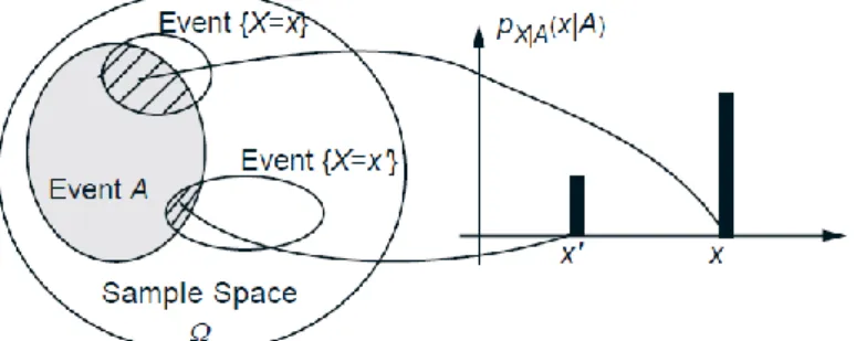
The conditional PMF is calculated similar to its unconditional counterpart: to obtain
𝑝𝑋|𝐴 𝑥 , we add the probabilities of the outcomes that give rise to 𝑋 = 𝑥 and belong to the
conditioning event 𝐴, and then normalize by dividing with 𝑃(𝐴) (see Fig. 1).
Figure 1: Visualization and calculation of the conditional PMF 𝑝𝑋|𝐴 𝑥 . For each 𝑥, we add the
probabilities of the outcomes in the intersection {𝑋 = 𝑥} ∩ 𝐴and normalize by diving with
𝑃(𝐴).
1.2 Conditioning one Random Variable on Another
Let 𝑋 and 𝑌 be two random variables associated with the same experiment. If we know
that the experimental value of 𝑌 is some particular 𝑦 (with 𝑝𝑌(𝑦) > 0), this provides partial knowledge about the value of 𝑋. This knowledge is captured by the conditional PMF 𝑝𝑋|𝑌 of 𝑋
given 𝑌, which is defined by specializing the definition of 𝑝𝑋|𝐴 to events 𝐴of the form {𝑌 = 𝑦}:
𝑝𝑋|𝑌(𝑥|𝑦) = 𝑃(𝑋 = 𝑥|𝑌 = 𝑦).
Using the definition of conditional probabilities, we have
𝑝𝑋|𝑌 𝑥 𝑦 =𝑃 𝑋=𝑥,𝑌=𝑦 𝑃 𝑌=𝑦 =𝑝𝑋 ,𝑌𝑝 (𝑥,𝑦)
𝑌(𝑦) .
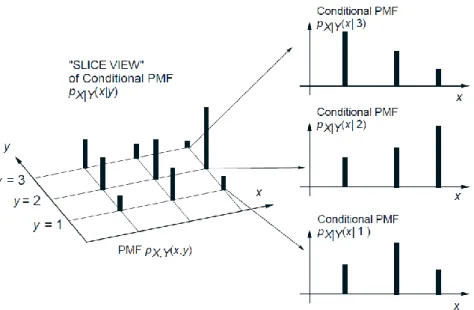
Let us fix some 𝑦, with 𝑝𝑌(𝑦) > 0 and consider 𝑝𝑋|𝑌 𝑥 𝑦 as a function of 𝑥. This
function is a valid PMF for 𝑋: it assigns nonnegative values to each possible 𝑥, and these values
add to 1. Furthermore, this function of 𝑥, has the same shape as 𝑝𝑋,𝑌(𝑥, 𝑦) except that it is
normalized by dividing with 𝑝𝑌(𝑦), which enforces the normalization property
Figure 2 provides a visualization of the conditional PMF.
Figure 2: Visualization of the conditional PMF 𝑝𝑋|𝑌 𝑥 𝑦 . For each 𝑦, we view the joint PMF
along the slice 𝑌 = 𝑦and renormalize so that 𝑝𝑥 𝑋|𝑌 𝑥 𝑦 = 1.
The conditional PMF is often convenient for the calculation of the joint PMF, using a
sequential approach and the formula
𝑝𝑋,𝑌 𝑥, 𝑦 = 𝑝𝑌(𝑦)𝑝𝑋|𝑌 𝑥 𝑦 ,
or its counterpart
𝑝𝑋,𝑌 𝑥, 𝑦 = 𝑝𝑋(𝑥)𝑝𝑌|𝑋 𝑦 𝑥 .
This method is entirely similar to the use of the multiplication rule.
Conditional Expectation
A conditional PMF can be thought of as an ordinary PMF over a new universe
determined by the conditioning event. In the same spirit, a conditional expectation is the same as
an ordinary expectation, except that it refers to the new universe, and all probabilities and PMFs
are replaced by their conditional counterparts. We list the main definitions and relevant facts
Summary of Facts About Conditional Expectations
Let 𝑋and 𝑌be random variables associated with the same experiment.
The conditional expectation of 𝑋given an event 𝐴with 𝑃(𝐴) > 0, is defined by
𝐸[𝑋|𝐴] = 𝑥𝑝𝑥 𝑋|𝐴(𝑥|𝐴).
For a function 𝑔(𝑋), it is given by
𝐸 𝑔(𝑋)|𝐴 = 𝑔(𝑥)𝑝𝑥 𝑋|𝐴(𝑥|𝐴).
The conditional expectation of 𝑋given a value 𝑦of 𝑌is defined by
𝐸[𝑋|𝑌 = 𝑦] = 𝑥𝑝𝑥 𝑋|𝑌(𝑥|𝑦).
We have
𝐸[𝑋] = 𝑝𝑦 𝑌(𝑦)𝐸[𝑋|𝑌 = 𝑦].
This is the total expectation theorem.
Let 𝐴1, 𝐴2, . . . , 𝐴𝑛 be disjoint events that form a partition of the sample space, and
assume that 𝑃(𝐴𝑖) > 0 for all 𝑖. Then,
𝐸[𝑋] = 𝑛 𝑃(𝐴𝑖)𝐸[𝑋|𝐴𝑖]
𝑖=1 .
1.3 Conditioning on a event (continuous RV)
The conditional PDF of a continuous random variable 𝑋, conditioned on a particular
event 𝐴with 𝑃(𝐴) > 0, is a function 𝑓𝑋|𝐴 that satisfies
𝑃(𝑋 ∈ 𝐵|𝐴) = 𝑓𝐵 𝑋|𝐴(𝑥)𝑑𝑥,
for any subset 𝐵of the real line. It is the same as an ordinary PDF, except that it now refers to a
An important special case arises when we condition on 𝑋 belonging to a subset 𝐴 of the
real line, with 𝑃(𝑋 ∈ 𝐴) > 0. We then have
𝑃(𝑋 ∈ 𝐵|𝑋 ∈ 𝐴) = 𝑃(𝑋∈𝐵 𝑎𝑛𝑑 𝑋∈𝐴)𝑃(𝑋∈𝐴) = 𝐴∩𝐵𝑓𝑋(𝑥)𝑑𝑥
𝑃(𝑋∈𝐴) .
This formula must agree with the earlier one, and therefore,
𝑓𝑋|𝐴(𝑥|𝐴) =
𝑓𝑋(𝑥)
𝑃(𝑋 ∈ 𝐴) 𝑖𝑓 𝑥 ∈ 𝐴, 0 𝑜𝑡𝑒𝑟𝑤𝑖𝑠𝑒.
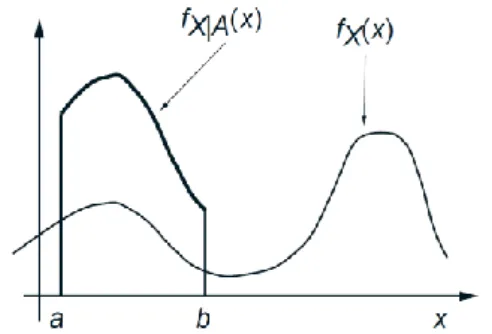
As in the discrete case, the conditional PDF is zero outside the conditioning set. Within
the conditioning set, the conditional PDF has exactly the same shape as the unconditional one,
except that it is scaled by the constant factor 1/𝑃(𝑋 ∈ 𝐴). This normalization ensures that 𝑓𝑋|𝐴
integrates to 1, which makes it a legitimate PDF; see Fig. 3.
Figure 3: The unconditional PDF 𝑓𝑋 and the conditional PDF 𝑓𝑋|𝐴, where A is the interval [𝑎, 𝑏].
Note that within the conditioning event 𝐴, 𝑓𝑋|𝐴 retains the same shape as 𝑓𝑋, except that it is
scaled along the vertical axis.
Conditional PDF and Expectation Given an Event
The corresponding conditional expectation is defined by
𝐸[𝑋|𝐴] = 𝑥𝑓−∞∞ 𝑋|𝐴(𝑥) 𝑑𝑥.
The expected value rule remains valid:
If 𝐴1, 𝐴2, . . . , 𝐴𝑛 are disjoint events with 𝑃(𝐴𝑖) > 0 for each 𝑖, that form a partition
of the sample space, then
𝑓𝑋(𝑥) = 𝑃(𝐴𝑖)𝑓𝑋|𝐴𝑖(𝑥)
𝑛
𝑖=1
(a version of the total probability theorem), and
𝐸[𝑋] = 𝑃(𝐴𝑖)𝐸[𝑋|𝐴𝑖] 𝑛
𝑖=1
(the total expectation theorem). Similarly,
𝐸 𝑔(𝑋) = 𝑛𝑖=1𝑃(𝐴𝑖)𝐸 𝑔(𝑋)|𝐴𝑖 .
2 Basic probability laws of continuous random variables
2.1 Unifrom Random Variable
2.1.1 Continuous Uniform Random Variable
A gambler spins a wheel of fortune, continuously calibrated between 0 and 1, and
observes the resulting number. Assuming that all subintervals of [0,1] of the same length are equally likely, this experiment can be modeled in terms a random variable 𝑋 with PDF
𝑓𝑋(𝑥) = 𝑐 𝑖𝑓 0 ≤ 𝑥 ≤ 1,0 𝑜𝑡𝑒𝑟𝑤𝑖𝑠𝑒,
for some constant 𝑐. This constant can be determined by using the normalization property
1 = 𝑓∞ 𝑋(𝑥)𝑑𝑥
−∞
= 𝑐𝑑𝑥1
0
= 𝑐 𝑑𝑥1
0
so that 𝑐 = 1.
More generally, we can consider a random variable 𝑋 that takes values in an interval
[𝑎, 𝑏], and again assume that all subintervals of the same length are equally likely. We refer to
this type of random variable as uniform or uniformly distributed. Its PDF has the form
𝑓𝑋(𝑥) = 𝑐 𝑖𝑓 𝑎 ≤ 𝑥 ≤ 𝑏, 0 𝑜𝑡𝑒𝑟𝑤𝑖𝑠𝑒,
where 𝑐 is a constant. This is the continuous analog of the discrete uniform random variable. For
𝑓𝑋 to satisfy the normalization property, we must have (cf. Fig. 2)
1 = 𝑐𝑑𝑥𝑏
𝑎
= 𝑐 𝑑𝑥𝑏
𝑎
= 𝑐 𝑏 − 𝑎
so that 𝑐 =𝑏−𝑎1 .
Note that the probability 𝑃(𝑋 ∈ 𝐼) that 𝑋 takes value in a set 𝐼 is
𝑃 𝑋 ∈ 𝐼 = [𝑎,𝑏]∩𝐼𝑏−𝑎1 𝑑𝑥= 𝑏−𝑎1 [𝑎,𝑏]∩𝐼𝑑𝑥 =𝑙𝑒𝑛𝑔𝑡 𝑜𝑓 [𝑎,𝑏]∩𝐼 𝑙𝑒𝑛𝑔𝑡 𝑜𝑓 [𝑎,𝑏] .
The uniform random variable bears a relation to the discrete uniform law, which involves
a sample space with a finite number of equally likely outcomes. The difference is that to obtain
the probability of various events, we must now calculate the “length” of various subsets of the
real line instead of counting the number of outcomes contained in various events.
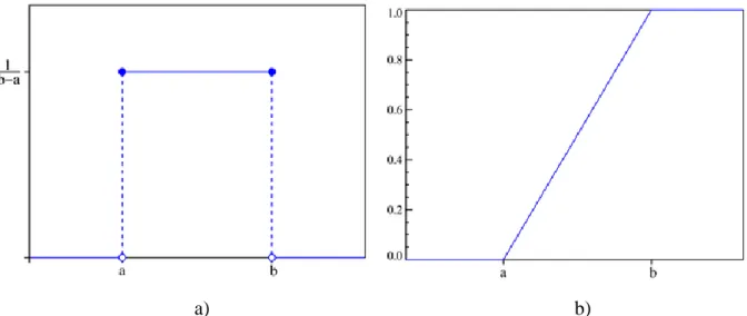
The CDF is
𝐹𝑋 𝑥 =
0 𝑓𝑜𝑟 𝑥 < 𝑎, 𝑥 − 𝑎
a) b)
Figure 4: Uniform Probability density function (a) and Cumulative distribution function (b)
Mean and Variance of the Uniform Random Variable
Consider the case of a uniform PDF over an interval [𝑎, 𝑏]. We have
𝐸 𝑋 = 𝑥𝑓−∞∞ 𝑋 𝑥 𝑑𝑥= 𝑥 ∙𝑎𝑏 𝑏−𝑎1 𝑑𝑥= 𝑏−𝑎1 ∙12𝑥2 𝑏𝑎 =𝑏−𝑎1 ∙𝑏
2−𝑎2
2 =
𝑎+𝑏 2 ,
as one expects based on the symmetry of the PDF around (𝑎 + 𝑏)/2.
To obtain the variance, we first calculate the second moment. We have
𝐸 𝑋2 = 𝑥2 𝑏−𝑎𝑑𝑥 𝑏
𝑎 =
1 𝑏−𝑎 𝑥
2𝑑𝑥 𝑏 𝑎 = 1 𝑏−𝑎∙ 1 3𝑥
3 𝑏
𝑎 =
𝑏3−𝑎3
3(𝑏−𝑎)=
𝑎2+𝑎𝑏 +𝑏2
3 .
Thus, the variance is obtained as
var 𝑋 = 𝐸 𝑋2 − 𝐸 𝑋 2 = 𝑎2+𝑎𝑏 +𝑏2
3 −
𝑎+𝑏 2
4 =
𝑏−𝑎 2
12 ,
after some calculation.
2.1.2 Discrete Uniform Random Variable
What is the mean and variance of the roll of a fair six-sided die? If we view the result of
𝑝𝑋(𝑘) = 1/6 𝑖𝑓 𝑘 = 1, 2, 3, 4, 5, 6, 0 𝑜𝑡𝑒𝑟𝑤𝑖𝑠𝑒.
Since the PMF is symmetric around 3.5, we conclude that 𝐸[𝑋] = 3.5. Regarding the variance, we have
var 𝑋 = 𝐸 𝑋2 − 𝐸 𝑋 2 =1 6(1
2+ 22 + 32+ 42 + 52+ 62) − (3.5)2,
which yields var(𝑋) = 35/12.
The above random variable is a special case of a discrete uniformly distributed random
variable (or discrete uniform for short), which by definition, takes one out of a range of
contiguous integer values, with equal probability. More precisely, this random variable has a
PMF of the form
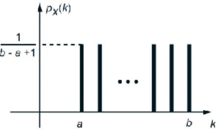
𝑝𝑋(𝑘) = 1
𝑏−𝑎+1 𝑖𝑓 𝑘 = 𝑎, 𝑎 + 1, … , 𝑏,
0 𝑜𝑡𝑒𝑟𝑤𝑖𝑠𝑒, ,
where 𝑎and 𝑏are two integers with 𝑎 < 𝑏. The mean is
𝐸[𝑋] =𝑎+𝑏2 ,
as can be seen by inspection, since the PMF is symmetric around (𝑎 + 𝑏)/2. To calculate the
variance of 𝑋, we first consider the simpler case where 𝑎 = 1 and 𝑏 = 𝑛. It can be verified by induction on 𝑛that
𝐸[𝑋2] = 1
𝑛 𝑘
2 𝑛
𝑘=1 =16(𝑛 + 1)(2𝑛 + 1).
We leave the verification of this as an exercise for the reader. The variance can now be
obtained in terms of the first and second moments
var(𝑋) = 𝐸[𝑋2] − 𝐸[𝑋] 2 =1
6(𝑛 + 1)(2𝑛 + 1) − 1
4(𝑛 + 1) 2 = 1
12(𝑛 + 1)(4𝑛 + 2 −
Figure 5: PMF of the discrete random variable that is uniformly distributed between two
integers 𝑎and 𝑏. Its mean and variance are
𝐸[𝑋] =𝑎+𝑏2 , var[𝑋] = 𝑏−𝑎 (𝑏−𝑎+2)12 .
For the case of general integers 𝑎 and 𝑏, we note that the uniformly distributed random variable over [𝑎, 𝑏] has the same variance as the uniformly distributed random variable over the
interval [1, 𝑏 − 𝑎 + 1], since these two random variables differ by the constant 𝑎 − 1. Therefore,
the desired variance is given by the above formula with 𝑛 = 𝑏 − 𝑎 + 1, which yields
var 𝑋 = 𝑏−𝑎+1 12 2−1 = 𝑏−𝑎 (𝑏−𝑎+2)12 .
a) b)
Figure 6: Discrete Uniform PDF (a) and CDF (b)
2.2 Exponential Random Variable
2.2.1 Exponential PDF and CDF
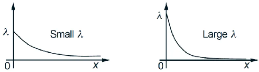
𝑓𝑋 𝑥 = 𝜆𝑒
−𝜆𝑥 𝑖𝑓 𝑥 ≥ 0,
0 𝑜𝑡𝑒𝑟𝑤𝑖𝑠𝑒,
where 𝜆 is a positive parameter characterizing the PDF (see Fig. 4). This is a legitimate PDF because
𝑓−∞∞ 𝑋(𝑥)𝑑𝑥 = 𝜆𝑒0∞ −𝜆𝑥𝑑𝑥= −𝑒−𝜆𝑥|0∞ = 1.
Note that the probability that 𝑋 exceeds a certain value falls exponentially. Indeed, for any 𝑎 ≥ 0, we have
𝑃(𝑋 ≥ 𝑎) = 𝜆𝑒∞ −𝜆𝑥𝑑𝑥
𝑎 = −𝑒−𝜆𝑥|𝑎∞ = 𝑒−𝜆𝑎.
An exponential random variable can be a very good model for the amount of time until a
piece of equipment breaks down, until a light bulb burns out, or until an accident occurs. It will
play a major role in study of random processes.
Figure 7: The PDF λe−λx of an exponential random variable.
The mean and the variance can be calculated to be
𝐸[𝑋] =1𝜆, var(𝑋) =𝜆12.
These formulas can be verified by straightforward calculation. We have, using integration
by parts,
𝐸[𝑋] = 𝑥𝜆𝑒∞ −𝜆𝑥𝑑𝑥
0 = (−𝑥𝑒−𝜆𝑥)|0∞ + 𝑒−𝜆𝑥𝑑𝑥
∞
0 = 0 −
𝑒−𝜆𝑥 𝜆 |0
∞ =1 𝜆.
𝐸[𝑋2] = 𝑥∞ 2𝜆𝑒−𝜆𝑥𝑑𝑥
0 = (−𝑥2𝑒−𝜆𝑥)|0∞+ 2𝑥𝑒−𝜆𝑥𝑑𝑥
∞
0 = 0 +
2
𝜆𝐸[𝑋] = 2 𝜆2.
Finally, using the formula var(𝑋) = 𝐸[𝑋2] − 𝐸[𝑋] 2, we obtain
var 𝑋 = 𝜆22−𝜆12 = 𝜆12.
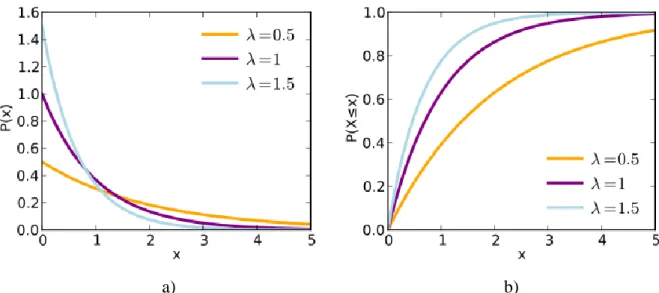
The cumulative distribution function is given by:
𝐹𝑋 𝑥 = 1 − 𝑒
−𝜆𝑥 𝑖𝑓 𝑥 ≥ 0,
0 𝑜𝑡𝑒𝑟𝑤𝑖𝑠𝑒.
Other moments:
Median: ln (2) 𝜆 .
Mode: 0. Skewness: 2.
Kurtosis: 6.
2.2.2 Memoryless property
An important property of the exponential distribution is that it is memoryless. This
means that if a random variable 𝑇 is exponentially distributed, its conditional probability obeys:
𝑃 𝑇 > 𝑠 + 𝑡 | 𝑇 > 𝑠 = 𝑃 𝑇 > 𝑡 𝑓𝑜𝑟 𝑎𝑙𝑙 𝑠, 𝑡 ≥ 0.
This says that the conditional probability that we need to wait, for example, more than
another 10 seconds before the first arrival, given that the first arrival has not yet happened after
30 seconds, is no different from the initial probability that we need to wait more than 10 seconds
for the first arrival. This is often misunderstood by students taking courses on probability: the
fact tha 𝑃(𝑇 > 40 | 𝑇 > 30) = 𝑃(𝑇 > 10)t does not mean that the events 𝑇 > 40 and 𝑇 > 30
are independent. To summarize: "memorylessness" of the probability distribution of the waiting
time 𝑇 until the first arrival means
It does NOT MEAN
𝑊𝑅𝑂𝑁𝐺 𝑃(𝑇 > 40 | 𝑇 > 30) = 𝑃(𝑇 > 40).
(That would be independence. These two events are NOT independent.)
The exponential distributions and the geometric distributions are the only memoryless
probability distributions.
a) b)
Figure 8: Exponential Probability density function (a) and Cumulative distribution function (b)
2.2.3 Occurrence and applications
The exponential distribution occurs naturally when describing the lengths of the
inter-arrival times in a homogeneous Poisson process.
The exponential distribution may be viewed as a continuous counterpart of the geometric
distribution, which describes the number of Bernoulli trials necessary for a discrete process to
change state. In contrast, the exponential distribution describes the time for a continuous process
to change state.
In real-world scenarios, the assumption of a constant rate (or probability per unit time) is
rarely satisfied. For example, the rate of incoming phone calls differs according to the time of
day. But if we focus on a time interval during which the rate is roughly constant, such as from 2
to 4 p.m. during work days, the exponential distribution can be used as a good approximate
In queuing theory, the service times of agents in a system (e.g. how long it takes for a
bank teller etc. to serve a customer) are often modeled as exponentially distributed variables.
Reliability theory and reliability engineering also make extensive use of the exponential
distribution. Because of the memoryless property of this distribution, it is well-suited to model
the constant hazard rate portion of the bathtub curve used in reliability theory. It is also very
convenient because it is so easy to add failure rates in a reliability model. The exponential
distribution is however not appropriate to model the overall lifetime of organisms or technical
devices, because the "failure rates" here are not constant: more failures occur for very “young”
and for very “old” systems.
2.3 Normal random variables
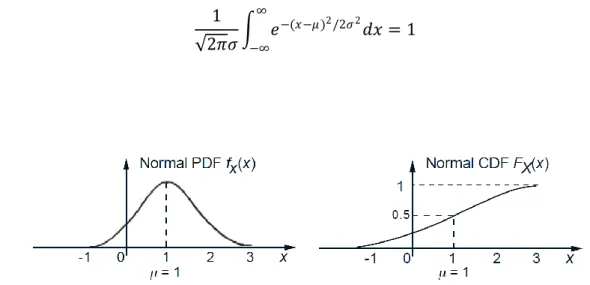
A continuous random variable 𝑋is said to be normal or Gaussian if it has a PDF of the form (see Fig. 9)
𝑓𝑋(𝑥) = 1
2𝜋𝜎𝑒
−(𝑥−𝜇)2/2𝜎2,
where 𝜇and 𝜎are two scalar parameters characterizing the PDF, with 𝜎assumed nonnegative. It can be verified that the normalization property
1
2𝜋𝜎 𝑒
−(𝑥−𝜇)2/2𝜎2𝑑𝑥 ∞
−∞
= 1
holds.
Figure 9: A normal PDF and CDF, with 𝜇 = 1 and 𝜎2 = 1. We observe that the PDF is
symmetric around its mean 𝜇, and has a characteristic bell-shape. As 𝑥gets further from 𝜇, the
The mean and the variance can be calculated to be
𝐸[𝑋] = 𝜇, var(𝑋) = 𝜎2.
To see this, note that the PDF is symmetric around 𝜇, so its mean must be 𝜇.
Furthermore, the variance is given by
var(𝑋) = 2𝜋𝜎1 (𝑥 − 𝜇)2𝑒−(𝑥−𝜇)2/2𝜎2
𝑑𝑥
∞
−∞ .
Using the change of variables 𝑦 = (𝑥 − 𝜇)/𝜎and integration by parts, we have
var 𝑋 = 𝜎2
2𝜋 𝑦
2𝑒−𝑦 22𝑑𝑦 ∞
−∞ = var 𝑋 =
𝜎2
2𝜋 −𝑦𝑒
−𝑦 22 ∞
−∞ +
𝜎2
2𝜋 𝑒
−𝑦 22𝑑𝑦 ∞
−∞ =
𝜎2
2𝜋 𝑒
−𝑦 22𝑑𝑦 ∞
−∞ = 𝜎2.
The last equality above is obtained by using the fact
1
2𝜋 𝑒
−𝑦 22𝑑𝑦 ∞
−∞ = 1,
which is just the normalization property of the normal PDF for the case where 𝜇 = 0 and 𝜎 = 1. The normal random variable has several special properties.
Normality is Preserved by Linear Transformations
If 𝑋 is a normal random variable with mean 𝜇 and variance 𝜎2, and if 𝑎, 𝑏 are scalars, then the random variable
𝑌 = 𝑎𝑋 + 𝑏
is also normal, with mean and variance
𝐸[𝑌] = 𝑎𝜇 + 𝑏, var(𝑌) = 𝑎2𝜎2.
A normal random variable 𝑌 with zero mean (𝜇 = 0) and unit variance (𝜎2 = 1) is said
to be a standard normal. Its CDF is denoted by Φ,
Φ(𝑦) = 𝑃(𝑌 ≤ 𝑦) = 𝑃(𝑌 < 𝑦) = 1
2𝜋 𝑒
−𝑡22𝑑𝑡 𝑦
−∞ .
It is recorded in a table, and is a very useful tool for calculating various probabilities
involving normal random variables; see also Fig. 10.
Note that the table only provides the values of Φ(𝑦) for 𝑦 ≥ 0, because the omitted values can be found using the symmetry of the PDF. For example, if 𝑌 is a standard normal
random variable, we have
Φ(−0.5) = 𝑃(𝑌 ≤ −0.5) = 𝑃(𝑌 ≥ 0.5) = 1 − 𝑃(𝑌 < 0.5) = 1 − Φ(0.5) = 1 − 0.6915 = 0.3085.
Let 𝑋be a normal random variable with mean 𝜇and variance 𝜎2. We “standardize” 𝑋by defining a new random variable 𝑌given by
𝑌 =𝑋−𝜇𝜎 .
Since 𝑌is a linear transformation of 𝑋, it is normal. Furthermore,
𝐸[𝑌] =𝐸[𝑋]−𝜇𝜎 = 0, var(𝑌) =var (𝑋)𝜎2 = 1.
Thus, 𝑌 is a standard normal random variable. This fact allows us to calculate the
Figure 10: The PDF 𝑓𝑌(𝑦) = 1 2𝜋𝑒
−𝑦2/2
of the standard normal random variable. Its
corresponding CDF, which is denoted by Φ(𝑦), is recorded in a table.
Generalizing the approach, we have the following procedure.
CDF Calculation of the Normal Random Variable
The CDF of a normal random variable 𝑋 with mean 𝜇 and variance 𝜎2 is obtained using the standard normal table as
𝑃(𝑋 ≤ 𝑥) = 𝑃 𝑋−𝜇𝜎 ≤𝑥−𝜇𝜎 = 𝑃 𝑌 ≤ 𝑥−𝜇𝜎 = Φ 𝑥−𝜇𝜎 ,
where 𝑌is a standard normal random variable.
The normal random variable is often used in signal processing and communications
engineering to model noise and unpredictable distortions of signals.
The normal random variable plays an important role in a broad range of probabilistic
models. The main reason is that, generally speaking, it models well the additive effect of many
independent factors, in a variety of engineering, physical, and statistical contexts.
Mathematically, the key fact is that the sum of a large number of independent and identically
distributed (not necessarily normal) random variables has an approximately normal CDF,
regardless of the CDF of the individual random variables. This property is captured in the
celebrated central limit theorem.
The standard normal CDF can be expressed in terms of a special function called the error
function, as
Φ(𝑦) =12 1 + erf 𝑦
2 .
Probability Content from
−∞
to
𝒁
z 0.00 0.01 0.02 0.03 0.04 0.05 0.06 0.07 0.08 0.09
0.0 0.5000 0.5040 0.5080 0.5120 0.5160 0.5199 0.5239 0.5279 0.5319 0.5359
0.1 0.5398 0.5438 0.5478 0.5517 0.5557 0.5596 0.5636 0.5675 0.5714 0.5753
0.2 0.5793 0.5832 0.5871 0.5910 0.5948 0.5987 0.6026 0.6064 0.6103 0.6141
0.4 0.6554 0.6591 0.6628 0.6664 0.6700 0.6736 0.6772 0.6808 0.6844 0.6879
0.5 0.6915 0.6950 0.6985 0.7019 0.7054 0.7088 0.7123 0.7157 0.7190 0.7224
0.6 0.7257 0.7291 0.7324 0.7357 0.7389 0.7422 0.7454 0.7486 0.7517 0.7549
0.7 0.7580 0.7611 0.7642 0.7673 0.7704 0.7734 0.7764 0.7794 0.7823 0.7852
0.8 0.7881 0.7910 0.7939 0.7967 0.7995 0.8023 0.8051 0.8078 0.8106 0.8133
0.9 0.8159 0.8186 0.8212 0.8238 0.8264 0.8289 0.8315 0.8340 0.8365 0.8389
1.0 0.8413 0.8438 0.8461 0.8485 0.8508 0.8531 0.8554 0.8577 0.8599 0.8621
1.1 0.8643 0.8665 0.8686 0.8708 0.8729 0.8749 0.8770 0.8790 0.8810 0.8830
1.2 0.8849 0.8869 0.8888 0.8907 0.8925 0.8944 0.8962 0.8980 0.8997 0.9015
1.3 0.9032 0.9049 0.9066 0.9082 0.9099 0.9115 0.9131 0.9147 0.9162 0.9177
1.4 0.9192 0.9207 0.9222 0.9236 0.9251 0.9265 0.9279 0.9292 0.9306 0.9319
1.5 0.9332 0.9345 0.9357 0.9370 0.9382 0.9394 0.9406 0.9418 0.9429 0.9441
1.6 0.9452 0.9463 0.9474 0.9484 0.9495 0.9505 0.9515 0.9525 0.9535 0.9545
1.7 0.9554 0.9564 0.9573 0.9582 0.9591 0.9599 0.9608 0.9616 0.9625 0.9633
1.8 0.9641 0.9649 0.9656 0.9664 0.9671 0.9678 0.9686 0.9693 0.9699 0.9706
1.9 0.9713 0.9719 0.9726 0.9732 0.9738 0.9744 0.9750 0.9756 0.9761 0.9767
2.0 0.9772 0.9778 0.9783 0.9788 0.9793 0.9798 0.9803 0.9808 0.9812 0.9817
2.1 0.9821 0.9826 0.9830 0.9834 0.9838 0.9842 0.9846 0.9850 0.9854 0.9857
2.2 0.9861 0.9864 0.9868 0.9871 0.9875 0.9878 0.9881 0.9884 0.9887 0.9890
2.3 0.9893 0.9896 0.9898 0.9901 0.9904 0.9906 0.9909 0.9911 0.9913 0.9916
2.4 0.9918 0.9920 0.9922 0.9925 0.9927 0.9929 0.9931 0.9932 0.9934 0.9936
2.5 0.9938 0.9940 0.9941 0.9943 0.9945 0.9946 0.9948 0.9949 0.9951 0.9952
2.6 0.9953 0.9955 0.9956 0.9957 0.9959 0.9960 0.9961 0.9962 0.9963 0.9964
2.7 0.9965 0.9966 0.9967 0.9968 0.9969 0.9970 0.9971 0.9972 0.9973 0.9974
2.8 0.9974 0.9975 0.9976 0.9977 0.9977 0.9978 0.9979 0.9979 0.9980 0.9981
2.9 0.9981 0.9982 0.9982 0.9983 0.9984 0.9984 0.9985 0.9985 0.9986 0.9986
3.0 0.9987 0.9987 0.9987 0.9988 0.9988 0.9989 0.9989 0.9989 0.9990 0.9990
Examples
A professor's exam scores are approximately distributed normally with mean 80 and
standard deviation 5.
What is the probability that a student scores an 82 or less?
𝑃(𝑋 ≤ 82) = 𝑃(𝑍 ≤ (82 − 80)/5) = 𝑃(𝑍 ≤ 0.40) = 0.6554.
𝑃(𝑋 ≥ 90) = 𝑃(𝑍 ≥ (90 − 80)/5) = 𝑃(𝑍 ≥ 2.00) = 1 − 𝑃(𝑍 ≤ 2.00) = 1 − 0.9772 = 0.0228.
What is the probability that a student scores a 74 or less?
𝑃(𝑋 ≤ 74) = 𝑃(𝑍 ≤ (74 − 80)/5) = 𝑃(𝑍 ≤ −1.2) = 0.1151.
If your table does not have negatives, use 𝑃(𝑍 ≤ −1.2) = 𝑃(𝑍 ≥ 1.2) = 1 − 0.8849 =
0.1151.
What is the probability that a student scores between 78 and 88?
𝑃(78 ≤ 𝑋 ≤ 88) = 𝑃((78 − 80)/5 ≤ 𝑍 ≤ (88 − 80)/5) = 𝑃(−0.4 ≤ 𝑍 ≤ 1.6) = 𝑃(𝑍 ≤ 1.6) − 𝑃(𝑍 ≤ −0.4) = 0.9452 − 0.3446 = 0.6006.
What is the probability that an average of three scores is 82 or less?
𝑃(𝑋 ≤ 82) = 𝑃(𝑍 ≤ (82 − 80)/(5/ 3)) = 𝑃(𝑍 ≤ 0.69) = 0.7549.
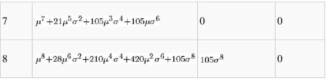
Order Raw moment Central moment Cumulant
1 0
2
3 0 0
4 0
5 0 0
7 0 0
8 0
About 68% of values drawn from a normal distribution are within one standard deviation
σ > 0 away from the mean μ; about 95% of the values are within two standard deviations and
about 99.7% lie within three standard deviations. This is known as the 68-95-99.7 rule, or the
empirical rule, or the 3-sigma rule.
Figure 4 Dark blue is less than one standard deviation from the mean. For the normal
distribution, this accounts for about 68% of the set (dark blue), while two standard deviations
from the mean (medium and dark blue) account for about 95%, and three standard deviations
(light, medium, and dark blue) account for about 99.7%.
In statistics, the 68-95-99.7 rule, or three-sigma rule, or empirical rule, states that for a
normal distribution, nearly all values lie within 3 standard deviations of the mean.
About 68% of the values lie within 1 standard deviation of the mean (or between the
mean minus 1 times the standard deviation, and the mean plus 1 times the standard deviation). In
statistical notation, this is represented as: 𝜇 ± 𝜎.
About 95% of the values lie within 2 standard deviations of the mean (or between the
mean minus 2 times the standard deviation, and the mean plus 2 times the standard deviation).
The statistical notation for this is: 𝜇 ± 2𝜎.
Nearly all (99.7%) of the values lie within 3 standard deviations of the mean (or between
the mean minus 3 times the standard deviation and the mean plus 3 times the standard deviation).
This rule is often used to quickly get a rough estimate of something's probability, given
its standard deviation, if the population is assumed normal, thus also as a simple test for outliers
(if the population is assumed normal), and as a normality test (if the population is potentially not