representing fuzzy temporal knowledge KBCS2000

Representing Fuzzy Temporal Knowledge

Girish Keshav Palshikar

Tata Research Development and Design Centre (TRDDC), 54B, Hadapsar Industrial Estate,

Pune 411013, India.

Email:[email protected]

Abstract

Many systems collect vast data over time, which is used for critical tasks like diagnosis, surveillance, resource management, planning and forecasting. To effectively use the historical data for these purposes, it is important to comprehend its significant structure by identifying the presence and characteristics of specific patterns. We describe a fuzzy logical notation, enhanced with facilities for expressing approximate temporal patterns, to build compositional and abstract models of syntactic structure of patterns. We describe how a temporal database can provide an interpretation for a given formula in this logic. We describe a fuzzy version of Allen’s interval algebra as meta-temporal facilities to specify intervals where a given fuzzy temporal formula shows a significant presence and to describe relationships between intervals. We illustrate this logic to describe fuzzy temporal patterns over temporal databases and to express expert knowledge about temporal phenomena; we use the problem of identifying failing and potentially failing banks from their operational data.

1

Introduction

Many software systems maintain vast temporal databases containing data about attributes at various specific times. The underlying structure of time (i.e., the instants, the beginnings and end of timeline etc.) is usually fixed and known in advance. Examples: stock market databases, banking, accounting, sales and purchase databases, billing and inventory databases, log of process control systems, telemetry data from dynamic systems (e.g., on-board systems in avionics and aero-space systems, power distribution systems etc.). Managers and other decision-makers often need to comprehend various qualitative patterns present in such data. They have considerable expertise in qualitatively stating frequently occurring patterns hidden inside these movement databases. They need tools to express and detect these patterns in given databases. Human beings are usually unable to comprehend the patterns in the enormous historical data in such systems. Our descriptions of such temporal data patterns are conceptually at a very high level of abstraction, away from table structure, keys etc. and is in terms of domain concepts. Moreover, we often use qualitative, approximate and probabilistic or fuzzy terms in English descriptions of such temporal patterns. Most users of temporal data would find it useful to be assisted by a system to help them query, automatically identify, state these patterns in a qualitative temporal pattern language that we can understand and to perform inferences and reasoning.

We sometimes need to represent information and expert knowledge involving temporal aspects of systems and physical phenomena. Often such temporal knowledge is also qualitative and approximate; examples: the stock price will eventually fall, the rains will continue until the pressure reduces, whenever the furnace temperature rises rapidly the yield quality deteriorates etc. Such temporal knowledge is qualitative in the sense that one does not specify actual time instants and intervals but deals with temporal relationships between events. It is approximate in that the statements may have

fuzzy (rather than Boolean) truth-values. We need a fuzzy temporal logical framework to state such

underlying temporal database can provide and interpretation for a given formula in this logic. Finally, we describe a fuzzy version of Allen’s interval algebra and how it can act as a meta-temporal facility for the fuzzy temporal logic and how it can be used to describe temporal knowledge.

Section 2 describes related work. Section 3 and 4 describe the fuzzy temporal logic and its semantics as also a fuzzy algebra for time intervals. Section 5 describes how fuzzy temporal patterns can be used to comprehend and analyse stock market trading databases. Section 6 discusses conclusions and further work.

2

Related Work

Qualitative reasoning is characterised by variables (which need not be Boolean), which take values from a small predetermined set. In contrast, we advocate the use of fuzzy logic in temporal reasoning and demonstrate how the underlying concepts can be modeled as fuzzy sets or fuzzy propositions. A major benefit of the fuzzy approach is the ability to model situations, which have multiple qualitative descriptions but with differing degree of strength. For example,, one can say that trading volume for a security is high with a degree of truth 0.8 and low with a degree of truth 0.36.

The ideas of incorporating fuzzy logic into the framework of temporal logic appeared in [Palshikar 2000] and [Kartalopoulos 2000], which differ in the temporal operators provided. Our work also contains new averaging temporal operators. The work of [Brusoni et al 1999] deals with specifying qualitative and quantitative temporal constraints over temporal databases. The need to use patterns, rather than precise queries and reports, for comprehending the data is well recognised to be important for effective management information systems [Inmon and Osterfelt 1991]. [Bardossy and Duckstein, 1995] discuss various applications of fuzzy rule-base systems, in particular to time series data. [Kirkland, Senator et al, 1999] discuss a similar approach for the stock market regulator application; their stress is on data mining and knowledge discovery and they have not used any formal fuzzy temporal logic framework. [Faloutos et al, 1994] discuss a more algorithmic approach to matching sub-sequences in time-series databases. [Shimakawa and Kikkawa, 1992] discuss an application of automatic trend recognition of time series databases to plant operations. The basic formalism of propositional linear temporal logic is in [Emerson, 1992] and crisp interval algebra is in [Allen 1984]. Coupling of logical languages with databases is an active area. [Parker 1990] discusses an interesting stream based approach to this problem. Our work is closely related to that in the temporal deductive databases, in particular, to TempLog and DatalogLS [Tansel, Clifford et al, 1993, Ch. 13]. For

specification and matching of simple patterns over databases, fuzzy (non-temporal) query languages ([Klir and Yuan, 1995], [Kacprzyk and Zadrozny, 1997], [Rasmussen and Yager, 1997]) can be used. Temporal query languages like TSQL, HSQL or TQuel [Tansel, Clifford et al, 1993, Ch. 4, 5, 6] can be used for (non-fuzzy) queries of temporal databases. [Maidchhi, Pernici and Barbie, 1992] provide a logic-based time calculus for temporal reasoning system over temporal databases.

3

Basic Notions

3.1

Notion of Time

Like fuzzy logic, we assume that the truth-value of a fuzzy proposition is a real number in the closed interval [0,1]. A fuzzy proposition is temporal if its truth-value varies from time to time and

non-temporal otherwise; e.g., high_price, low_volume are fuzzy non-temporal propositions. Let FZPROP be a

equally separated; TIME = <t0, t1, …, tN>, where N+1 is the number of time instants, each ti is a time

instant (0 ≤ i ≤ N) and ti < tj if i < j, for all 0 ≤ i, j ≤ N. For example <1, 3, 6, 7, 9, 12, 15> is a time

domain containing 7 time instants, where t0 = 1, t3 = 7 and t6 = 15. The special time variable (not a

temporal proposition) now or current-instant refers to some specific instant in TIME. A more detailed structure of the time domain is defined using several relations on TIME. For example, a linear ordered

timeline is defined by means of the usual Boolean relational operations (which are binary relations) R

= { <, =, >, ≤, ≥, ≠ } defined on TIME. For instance, ti < tj is true if the time point ti denotes a time

before the time denoted by the time-point tj. Note that our assumption that TIME is a given finite

sequence implies that we consider only a finitely interpreted logic. This is an important point and allows interpretation of formulae over finite temporal databases. By convention we denote t0 and tN its

minimum and maximum element respectively. A time interval is a tuple I = [ti, tj] = {ti, ti+1, …, tj-1, tj}

of time instants such that ti≤ tj. The length |I| of the time interval I = [ti, tj], is the natural number tj – ti

whereas the cardinality of I, denoted #I, is the number of time points tk in TIME such that ti≤ tk≤ tj.

Note that #I is always at least 1.

3.2

Fuzzy Interval Algebra

Allen’s interval algebra provides 13 possible (crisp) binary relations between time intervals. There are several ways to fuzzify them. An obvious way is to treat each time interval as a fuzzy set subset of TIME whose degree of membership function is given by something like a trapezoidal function. Another approach can treat each time instant as a fuzzy number. The laws of fuzzy arithmetic can then be used to given a fuzzy semantics for the 13 binary operations in the algebra. We propose another way to fuzzify these relationships. Essentially, we keep the underlying intervals to be crisp and re-define each crisp binary relation in the algebra as a fuzzy binary relation over the set of all crisp intervals over TIME. Each such fuzzy binary relation associates a fuzzy degree of truth with a tuple of crisp intervals. The main idea behind our approach is to regard ∧ and ∨ as fuzzy connectives and to provide an appropriate fuzzification for the relational operators. By the well-known correspondence

principle in fuzzy logic, we require that every such fuzzy binary relation should return a truth-value of

1 when the corresponding crisp relation holds between the given two intervals. For example, X fz_equals Y should be 1 when X equals Y. We can also suitably extend the semantics of these relations when either the first or second argument (but not both) is a time instant by considering an instant a as an interval [a,a]; e.g., a before [c,d] if a < c; a meets [c,d] if a+1 = c; a during [c,d] if a > c ∧ a < d; a after [c,d] if a > c etc.

We define parameterised fuzzy versions of the relational operators for positive integers (i.e., time

instants, in our case). The crisp binary relation a < b is replaced by a fuzzy less than relation a m b,

defined as follows: if a < b then a m b = 1 else a m b = µL(a,b-1,b+m), where the parameter m is a

given positive integer constant. The L-membership function is shown in Figure 1(a). For example, 5

3 6 = 1; 6 3 6 = µL(6,5,9) = 0.75; 7 3 6 = 0.5. The crisp binary relation a = b is replaced by a fuzzy equality relation a m,n b, defined as follows: if a = b then a m,n b = 1 else a m,n b = µ∆

(a,b-m,b,b+n), where the parameters m and n are given positive integer constants. The ∆-membership function is shown in Figure 1(c); e.g., 6 3,3 6 = 1; 5 3,3 6 = µ∆(5,2,6,9) = 0.75; 7 3,3 6 = 0.5. Other

corresponding fuzzy relational operators are defined as follows, where we assume the standard fuzzy semantics for the logical connectives ¬, ∧, ∨.

a m b =def (b m a)

a m b =def (a m b) ∨ (a m,m b)

a m,n b =def ¬(a m,n b)

Note that each of these fuzzy relations have an associated degree of membership function; e.g., the membership function for fuzzy greater than relation a >m b corresponds to the S-membership function

in Figure 1(b). It is easy to verify some common laws that hold for the fuzzy relational connectives; e.g., a m,n b = b n,m a, for all a, b. Moreover, the relational operators always return 1 whenever the

corresponding crisp relation holds between the arguments; e.g., a m b = 1 whenever a > b.

α β α β α β γ

µL(x,α,β) = 1 if x ≤α µS(x,α,β) = 0 if x ≤α µ∆(x,α,β,γ) = 0 if x ≤α

= 0 if x ≥β = 1 if x ≥β = 0 if x ≥γ = 1 – ((x - α) / (β - α)) = (x - α) / (β - α) = (x-α)/(α-β) if α < x < β = 1–((x-β)/(γ-β)) if β<x<γ

(a) L membership (b) S membership (c) Triangle membership

Figure 1. Some common membership functions; x, α, β are time instants from TIME.

Table 1. Fuzzification of the Thirteen Relations in Allen’s Interval Algebra

[a,b] fz_before [c,d]

b |d-b| c

[a,b] fz_meets [c,d]

b+1 b+1-a,d-c c

[a,b] fz_overlaps [c,d]

(a |d-a| c) ∧ (b |d-b| c) ∧ (b d-c d)

[a,b] fz_during [c,d]

(a |d-a| c) ∧ (b d-c d)

[a,b] fz_ starts[c,d]

(b d-c d) ∧ (a |d-a|,|d-a| c)

[a,b] fz_finishes [c,d]

(a |d-a| c) ∧ (a d-c d) ∧ (b |b-c|,|b-c| d)

[a,b] fz_equals [c,d]

(a |d-a|,|d-a| c) ∧ (b |b-c|,|b-c| d)

[a,b] fz_after [c,d]

[a,b] fz_met_by [c,d]

[c,d] fz_meets [a,b] [a,b] fz_overlapped_by [c,d]

[c,d] fz_overlaps [a,b] [a,b] fz_contains [c,d]

[c,d] fz_during [a,b] [a,b] fz_started_by [c,d]

[c,d] fz_starts [a,b] [a,b] fz_finished_by [c,d]

[c,d] fz_finishes [a,b]

additional fuzzy binary relations between intervals can also be defined. For instance, we can compute the strength of overlap of two intervals [a,b] and [c,d] as:

[a,b] fz_overlaps1 [c,d] = (b-c) / (d-a) if [a,b] overlaps [c,d] or [a,b] finishes [c,d]

= 0 otherwise

Then, for example, [10,20] fz_overlaps1 [18,30] = (20 – 18) / (30-10) = 2/20 = 0.1 and [10,20] fz_overlaps1 [12,20] = (20-12) / (20-10) = 8/10 = 0.8. For both these examples, fz_overlap returns a value 1, since the given intervals do actually overlap.

4

A Fuzzy Propositional Linear Temporal Logic

4.1

Syntax

Let FZPROP denote a finite non-empty set of given fuzzy propositional symbols. Let a, b ∈ TIME, p

∈ FZPROP, α ∈ [0,1] and F, G denote arbitrary fuzzy temporal formulae. The fuzzy temporal formulae, typically denoted by F, G etc., are inductively constructed as follows using fuzzy logic connectives ¬, ∧, ∨ and fuzzy temporal connectives in Table 2.

F ::= p | ¬F | F ∧ G | F ∨ G | ψ | Ψ | op F | F op G

where op is a unary or binary fuzzy temporal operator in Table 2

Example: Let c, h and r respectively denote the fuzzy propositions that it is cool, humid or raining. Let

heavy, fairly, low, high, very be user-specified unary fuzzy connectives. Then the statement “If it is

fairly cool and very humid then it will eventually rain within 5 minutes” is represented by the formula (fairly c ∧ very h) → ( 5 r) and the statement “If it is currently raining heavily then the rain will reduce

to a drizzle before eventually stopping” is represented by the formula (heavy r) → ((very low r) B ( (¬r))).

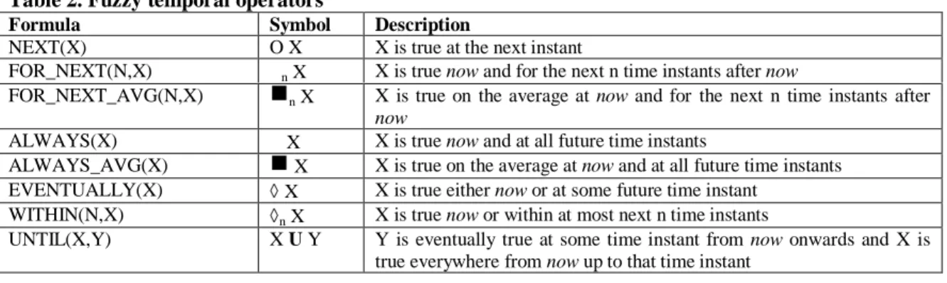
Table 2. Fuzzy temporal operators

Formula Symbol Description

NEXT(X) O X X is true at the next instant

FOR_NEXT(N,X) n X X is true now and for the next n time instants after now

FOR_NEXT_AVG(N,X) n X X is true on the average at now and for the next n time instants after now

ALWAYS(X) X X is true now and at all future time instants

ALWAYS_AVG(X) X X is true on the average at now and at all future time instants EVENTUALLY(X) X X is true either now or at some future time instant

WITHIN(N,X)

n X X is true now or within at most next n time instants

UNTIL(X,Y) X U Y Y is eventually true at some time instant from now onwards and X is true everywhere from now up to that time instant

4.2

Semantics

We now define methods to compute the truth-value of a given fuzzy temporal formula under a given interpretation. Let TIME = <t0, t1, …, tN> denote a given finite, linearly ordered timeline containing

timestamps occurring in given temporal databases, where ti < ti+1 for 0 ≤ i < N. A finite fuzzy temporal interpretation I:TIME×FZPROP→[0,1] is a total function which associates a fuzzy truth-value with every fuzzy proposition from the set FZPROP at every time instant in TIME i.e., I(ti,pj) = the truth

value of the fuzzy proposition pj ∈ FZPROP at the time instant ti in TIME, t0 ≤ ti ≤ tN. Given an

interpretation I and a fuzzy temporal formula F, the truth-value TV(F) of F in I at a time instant ti is

• TV(p) at ti = I(ti, p)

• TV(F ∧ G) at ti = min( TV(F) at ti, TV(G) at ti) • TV(F ∨ G) at ti = max( TV(F) at ti, TV(G) at ti) • TV(¬F) at ti = 1 - TV(F) at ti

• TV(F → G) at ti = TV(¬F ∨ G) = max( (1 - TV(F) at ti), TV(G) at ti) • TV(O F) at ti = TV(F) at ti+1 if i < N; TV(O F) at tN = false • TV( F) at ti = TV(F) at ti∧ TV(F) at ti+1∧ … ∧ TV(F) at tN

• TV( n F) at ti = TV(F) at ti∧ TV(F) at ti+1∧ … ∧ TV(F) at tk = min(TV(F) at ti, TV(F) at ti+1, …,

TV(F) at tk) where if i+n≤ N then k = i+n else k=N

• TV( F) at ti = TV(F) at ti∨ TV(F) at ti+1∨ … ∨ TV(F) at tN = max(TV(F) at ti, TV(F) at ti+1, …,

TV(F) at tN)

• TV( n F) at ti = TV(F) at ti∨ TV(F) at ti+1∨ … ∨ TV(F) = max(TV(F) at ti, TV(F) at ti+1, …,

TV(F) at tk) at tk where if i+n≤ N then k = i+n else k=N

• TV( F) at ti = [TV(F) at ti + TV(F) at ti+1 + … + TV(F) at tN] / (N – i + 1)

• TV( n F) at ti = [TV(F) at ti + TV(F) at ti+1 + … + TV(F) at tk] / m where if i+n≤ N then k = i+n

else k=N and m = (k – i + 1)

• TV(F U G) at ti = TV(G) at tk∧ TV(F) at ti∧ TV(F) at ti+1 ∧ … ∧ TV(F) at tk where the time

instant tk is such that ti≤ tk≤ tN and G achieves its maximum value at tk and there is no instant tj

strictly before tk such that TV(G) at tj = TV(G) at tk (i.e., tk is the maximum of G closest to ti) • TV(F B G) at ti = TV(G) at tk∧ TV(F) at ti∧ TV(F) at ti+1 ∧ … ∧ TV(F) at tk where the time

instant tk is such that ti≤ tk≤ tN and G achieves its maximum value at tk and there is no instant tj

strictly before tk such that TV(G) at tj = TV(G) at tk (i.e., tk is the maximum of G closest to ti) • TV(F at_time tj) at ti = TV(F) at tj

Intuitively, the formula F is true at time instant ti, if F is true at ti and F is true at ti+1 and … and F is

true at tN. The meaning of other future temporal operators can be easily understood similarly. Due to

these definitions, since ∧, ∨ are fuzzy connectives, so are the temporal operators in Table 2. Note that if TV( F) = 0.0 if there is even one instant where TV(F) = 0, even though F may have very high values at other instants in future. To reduce the influence of such outliers, we can use the averaging

and fuzzy connective defined (in the simplest case) by TV(F ∧ G) = [TV(F) + TV(G)] / 2. However, the averaging and connective is not associative. Table 2 contains new fuzzy temporal averaging operators , n, - and -n which act upon a time interval. The meaning of fuzzy temporal

connectives in Table 2 can be defined in other ways to take into account the difference between the instants, rather than implicitly treat all instants as equidistant. Moreover, it is possible to define variations of the connectives like n that refer to time length rather than number of instants.

4.3

Instant and Interval Formulae

Let FZPROP denote a finite non-empty set of given fuzzy propositional symbols. Let a, b ∈ TIME, p

∈ FZPROP, α∈ [0,1] and F, G denote fuzzy temporal formulae. An instant term, typically denoted by i, j etc., refers to a specific crisp time instant in TIME. An instant term can be specified as:

(i) an actual time instant in TIME (e.g., as an integer); or

(ii) special constants first_instant or last_instant, which refer to the end-points of the timeline and first_instant < last_instant; or

(iii) functions next_instant(i) and prev_instant(i) which refer to the next and the previous time instant from the given instant i;

(iv) [F]α which denotes a time instant (or equivalently, a one point time interval) where the

temporal formula F achieves a truth-value ≥α; or

(v) [F]-α which denotes a time instant (or equivalently, a one point time interval) the temporal

formula F achieves a truth-value ≥α.

Usual relational operators can be applied to instant terms to construct crisp Boolean instant formulae, typically denoted by ψ. Also, a formula F at_time i denotes the fuzzy truth-value of the formula F at a given time instant i.

i ::= a | now | first_instant | last_instant | next_instant(i) | prev_instant(i) | [F]α | [F]-α

ψ ::= i = j | i < j | i > j | F at_time i

A basic interval term, typically denoted by I, J etc., refers to a specific crisp time interval over in TIME. A basic interval term is specified as an actual time interval over TIME (e.g., as a tuple [ti,tj] of

instant terms, where ti, tj are instant terms and ti < tj). We introduce a general interval term [[F]]α where

F is a fuzzy temporal formula and threshold α∈ [0, 1]; the value of this interval term (i.e., the time interval denoted by this term) is computed as follows. If there exists a maximally extended time interval [ti, tj] (where ti, tj∈ TIME and ti < tj) such that

β = ([ TV(F) at ti + TV(F) at ti+1 + … + TV(F) at tj ] / n )

where TV(F) at i stands for the fuzzy truth-value of F at time instant i and n is the number of time instants in the interval [ti, tj] and β≥α, then the value of the interval term [[F]]α is the interval [ti, tj]; if

no such interval exists then the interval term refers to a special null interval, say [0,0]. The interval denoted by the interval term [[F]]α is maximally extended in the sense that no time instant can be added

to it (say tj+1) without reducing the average value of F over the extended to interval to less than α. We

define the covering interval of two given intervals [a,b] and [c,d], denoted cover([a,b], [c,d]) or [a,b],[c,d], as another interval [x,y] where x = min(a,c) and y = max(c,d). For example,

cover([20,30], [25,45]) = [20,45] and cover([10,20], [30,40]) = [10,40].

The intervals denoted by the interval terms are compared using interval algebra operators (Table 2) as well using logical (non-temporal) operators ¬, ∧ and ∨ into crisp or fuzzy interval formulae. In addition, a number of unary fuzzy operators like long, short, very, rather etc. can be applied to interval terms to yield fuzzy truth-values. For example, the truth-value of the fuzzy formula long([x,y]) can be defined to be (y – x) / (last_instant - first_instant).

I ::= [i, j] where i < j

For example, consider a situation in stock market where the share price is steady and the trading volume is low for a long time. This is followed by a short time period in which the trading volume is high and the share price is increasing. Assuming appropriately defined fuzzy temporal propositions, the above pattern can be expressed as follows:

[x1,y1] = [[price_steady ∧ volume_low]]0.8∧ long([x1,y1]) ∧

[x2,y2] = [[volume_high ∧ price_increasing]]0.9∧ short ([x2,y2]) ∧ [x1,y1] before [x2,y2]

The truth-value of the instant and interval formulae is computed as follows:

• TV(i op j) at ti = i op j where i, j are instant terms and op is a relational operator =, <, > etc. • TV(I op J) at ti = I op J where I,J are interval terms, op is a crisp binary relation from Table 1 • TV(I op J) at ti = I op J where I,J are interval terms, op is a fuzzy binary operator from Table 1

• TV( long([x,y]) ) at ti = (y – x) / (last_instant – first_instant)

5

Example

This section, we define some sample patterns useful for identifying failing and potentially failing banks; this section is partly based on [Alam et al, 2000], which used fuzzy clustering on non-temporal data for these tasks. During 1985-1992, over 1200 banks failed in USA and the estimated losses are about US$30 billion. In 1989 alone, 206 banks closed in USA and the cost to taxpayers was about US$6 billion. These failures can be attributed to factors like regulatory changes, changes in the markets, increased competition and more aggressive and riskier banking practices, particularly in the lending behaviour of banks. Stringent bank examination and control standards and increases risk aversions are necessary. Identification of failing banks as well as early warning for potentially failing banks by examining historical data are important tasks in this context. For this purpose, one needs to work with a temporal database containing a summary of the banking activities (compiled every month, say) and having a broad structure like that shown in the highly simplified table below. In addition, there may be a large number of tables containing details of various kinds (e.g., details of loans).

Time stamp

BankID Total assets

Total loans

Non-performing loans

Net loan losses

Net income

Provision for loan losses

Non-performing loans include loans due for more than 90 days and non-accrual loans. Rates of change can be defined on all these columns e.g., rate of change of total loans. Additional financial parameters (features) are well-known in the financial domain; e.g.,

NITA = (Net income) ÷ (Total assets)

NLLAA = (Net loan losses) ÷ (total assets – total loans i.e., adjusted assets) NPLTA = (Non-performing loans) ÷ (Total assets)

NLLTL = (Net loan losses) ÷ (Total loans)

NLLPLLNI = (Net loan losses + Provision for loan losses) ÷ (Net income)

NPLTA but steady values for NLLPLLNI is specified by the formula [[very high NLLTA ∧ very high NPLTA ∧ steady NLLPLLNI]]0.9. Interval operators can be used to specify relationships between such

intervals. We define some more fuzzy temporal patterns to characterize failing or poorly performing banks, although we leave out the precise formulae in the fuzzy temporal logic in this paper.

(i) Most of its non-performing loans eventually become loan losses.

(ii) Large increases in total loans within short time along with only small changes in provision for loan losses are followed by a period of high net loan losses.

6

Conclusions and Further Work

In this paper, we described a fuzzy temporal logic where a formula has a truth-value at each instant in time (computed from the given underlying temporal databases) and is useful to characterize time dependent phenomena. We described a fuzzy version of Allen’s interval algebra as interval based meta-temporal facilities to specify intervals where a given fuzzy temporal formula shows a significant presence. These facilities are also useful to describe relationships between various intervals of interests. We are building a prototype tool called SNIFFER, which incorporates a pattern specification mechanism based on the logic described in this paper. We are planning to use SNIFFER for a number of different applications like stock market trading surveillance, diagnostic fault patterns in telemetry data, operational risk monitoring using financial and accounting data etc. In such applications, an end user is interested in specifying and detecting important fuzzy temporal patterns for specific decision-making and purposes. The logic in this paper appears to be succinct and well suited to describe fuzzy temporal patterns over temporal databases and express knowledge about temporal phenomena. For further work, we wish to use SNIFFER in more applications and compare it to other techniques: data mining, clustering, machine learning, temporal queries etc.

Acknowledgements

I sincerely thank Prof. Mathai Joseph for his enthusiastic support. I thank Prof. K. V. Nori, Dr. C. Anantaram and TRDDC colleagues for discussions and feedback. Thanks to the referees for thorough review comments. Finally, I would like to thank Dr. Manasee Palshikar for her patience, hope and confidence in spite of many difficult obstacles.

References

[Alam et al, 2000]

Alam P., Booth D., Lee K., Thordarson T. The use of Fuzzy Clustering Algorithm and Self-organizing Neural Networks for identifying Potentially Failing Banks: an Experimental Study, Expert Systems with Applications, 18(3), April 2000, pp. 185-200.

[Allen, 1984]

Allen J.F. Towards a General Theory of Action and Time. AI, 23(2), 1984, pp. 123-154. [Bardossy and Duckstein, 1995]

Bardossy A., Duckstein L. Fuzzy Rule-based Modeling with Applications to Geophysical, Biological and Engineering Systems. CRC Press, 1995.

[Brusoni et al, 1999]

Brusoni V., Console L., Terenziani P., Pernici B. Qualitative and Quantitative Constraints and Relational Databases: Theory, Architecture and Applications. IEEE Trans. Knowledge Data Engg., vol. 11, no. 6, Nov-Dec., 1999, pp. 948-968.

[Emerson, 1992]

[Faloutos et al, 1994]

Faloutos C., Ranganathan M., Manolopoulous Y. Fast Sub-sequence Matching in Time Series Database, Proc. 1994, ACM SIGMOD.

[Inmon and Osterfelt, 1991]

Inmon W.H. and Osterfelt S. Understanding Data Pattern Processing. QED Technical Publishing Group, 1991. [Kacprzyk and Zadrozny, 1997]

Kacprzyk J. and Zadrozny S. Fuzzy Queries in Microsoft Access V.2. In Fuzzy Information Engg., D. Dubois, H. Prade, R.R. Yager (eds), John Wiley, 1997, pp. 223-232.

[Kartalopoulos, 2000]

Kartalopoulos S.V. Understanding Neural Networks and Fuzzy Logic. Prentice-Hall, 2000. [Kirkland et al, 1999]

Kirkland J.D., Senator T.E., Hayden J.J., Dybala T., Goldberg H.G., Shyr P. The NASD Regulation Advanced Detection System (ADS). Proc. Spring 1999 AAAI Conf., pp. 55-67.

[Maidchhi et al, 1992]

Maidchhi R., Pernici B., Barbie F. Automatic Deduction of Temporal Information. ACM Trans. Database Systems. Vol. 17, No. 4, Dec. 1992, pp. 647-688.

[Palshikar, 2000]

Palshikar G.K. A Fuzzy Temporal Notation and Its Application to Specify Fault Patterns in Diagnosis. Accepted for publication in Pattern Recognition Letters.

[Parker, 1990]

Parker D.S. Stream Data Analysis in Prolog. In Sterling L. (ed.), The Practice of Prolog, pp. 249-302, MIT Press, 1990.

[Ramussen and Yager, 1997]

Rasmussen D., Yager R.R. A Fuzzy SQL Summary Language for Data Discovery. In Fuzzy Information Engg., D. Dubois et al (eds), John Wiley, 1997, pp. 253-264.

[Shimakawa and Kikkawa, 1992]

Shimakawa H., Kikkawa K., 1992. Trend Recognition with Time Series Database. Proc. 2nd _{Far-east work. on}

Future Database Systems (Future Databases ’92), World Scientific. [Tansel et al, 1993]