Effect of routing flexibility on the performance of manufacturing system
Khan, W.U.a, Ali, M.b
a Department of Mechanical Engineering, AMU, Aligarh, India.
b Mechanical Engineering Section, University Polytechnic, AMU, Aligarh, India. a [email protected], b [email protected]
Abstract: This work presented in this paper is based on the simulation of the routing flexibility enabled manufacturing system. In this study four levels of each factor (i.e. routing flexibility, system load conditions, system capacity and four part sequencing rules) are considered for the investigation. The performance of the routing flexibility enabled manufacturing system (RFEMS) is evaluated using three performance measures like make-span time, resource utilization and work-in-process. The analysis of results shows that the performance of the manufacturing system may be improved by adding in routing flexibility at the initial level along with other factors. However, the benefit of this flexibility diminishes at higher levels of routing flexibilities.
Key words: Flexibility, Flexible manufacturing system, Routing flexibility, Makespan, Work-in-process, Resource utilization.
1. Introduction
In the present global market, manufacturers are facing vastly competitive, complex and dynamic industrial environment. The manufacturing performance is not only governed by the price of the product but other factors such as flexibility, quality, and delivery also have grate importance. Thus the researchers are focused on the additional advantages of the advance technologies like computer integration in manufacturing systems, automated material handling system, robotic arms and flexible manufacturing system (FMS). The most important advantage of these systems that are taken by the manufacturers is inherent flexibilities in these systems Gustavsson (1984).
Flexibility in any manufacturing system described as the ability of a system to react in an economic way for volume change, mix requirement, status of the machine and processing capabilities. There are several types of flexibilities mentioned in literature. Sethi and Sethi (1990) recognize flexibility as a multi-dimensional notion within the
manufacturing domain. Flexibility may be reactive or proactive in nature (Gerwin, 1993). Joseph and Sridharan (2012) studied the effect of routing flexibility, sequencing flexibility and sequencing rules of a perfect flexible manufacturing system on different performance measures. The flexibility is broadly classified as hardware flexibility and software flexibility Blackburn and Millen (1986). The later type of flexibility refers to the routing flexibility where as the software flexibility refers as sequencing flexibility. In routing flexibility there are options for the parts to move to one machine or other. It exists when the machines are capable to perform different type of operations without major change in the machine setup. Therefore in this paper we consider routing flexibility in place of sequencing flexibility.
Much of the work has been done on routing flexibility in the deterministic environment. The work focused the impact of routing flexibility with different performance measures in a stochastic environment of a routing flexibility enabled manufacturing system (RFEMS). Various measures are used to evaluate
the performance of RFEMS like make-span time, average resource utilization and work-in-process of parts. Taguchi principle is used to design the simulation experiments and results are statistical analyzed. The objectives of this paper are:
- To examine the interaction among different factors as routing flexibility, system capacity, system load condition, and part sequencing rules in a perfect RFEMS in a stochastic environment. - To find out the effect of various factors and their
levels on the performance of routing flexibility enabled manufacturing system.
This paper is organized as; section 2 represents the work background. Description of proposed RFEMS is presented in section 3. A brief explanation of the operational logic of the RFEMS model is presented in section 4. The section 5 describes the experiment design and methodology of the work. Results and discussion are presented in section 6 and 7 respectively. Finally, conclusions are given in Section 8.
2. Background and Motivation
In the past, much of the work has been done on routing problems with deterministic manufacturing environment and different solutions are proposed for the effectual control of system. But, very few researchers addressed the impact of routing flexibility on FMS with stochastic environment. Some of the researches and their findings are discussed here. Browne et al. (1984) defined routing flexibility is exposed when there is a breakdown of machine. They provide a good discussion on the routing flexibility and their impact on the manufacturing system. This reduces the lead-time and fractional decrease in the total job make-span using alternative routes. Pankaj et al. (1991) incorporates the reliability of machines to study routing flexibility. Zhao et al. (2001) considers genetic algorithm to the scheduling of flexible manufacturing systems with multiple routes. Barad et al. (2003) stated that routing flexibility is the means of processing parts through different routes in the system. But the setup time is a significant part of the lead time. Therefore routing flexibility shows significant impact on manufacturing lead time Wahab (2005). There are various manufacturing flexibilities mentioned in the literature but Chen et al. (2006) stated that all the manufacturing-related flexibilities are derived by the routing flexibility in the FMS. Wadhwa et al. (2008) worked over the impact of
routing flexibility on system performance with various planning and control strategies in an FMS. Ali and Wadhwa (2010) revels that, the increase in the routing flexibility level may not be treated as a key role in system performance enhancement. Mehdi et al. (2013) presents how the meta-heuristics (i.e. ant colony optimization, genetic algorithms, simulated annealing tabu search etc.) are adopted to solve the alternative route selection problem with real time so as to decrease the congestion in the manufacturing system. Hence we observe from literature review that introduction of flexibility, mainly routing flexibility, has been found to have helped firms in the reduction of lead time, bottlenecks and uncertainties.
A stochastic model was developed by Savsar and Aldaihani (2012) which expresses the system by the use of study state differential equations that are solved by MAPLE software and analyze performance measures of FMS under various operational conditions. This model is useful for researchers to analyze a manufacturing system. Rohit et al. (2016) were discussed the unforeseen situations in manufacturing systems like deadlock, machine breakdowns etc. and strived to overcome the impact of uncertainties. They also studied the scheduling of parts and their affect on the performance of manufacturing system. And developed an extrapolative schedule that takes care of the interruption in the system and maintain the performance of the manufacturing system.
Our study here explicitly find outs the impact of routing flexibility, system capacity, system load conditions and sequencing rules on the performance of a RFEMS with respect to make-span time, average resource utilization and work-in-process under stochastic manufacturing environment.
3. Description of RFEMS
This study is carried out on routing flexibility enabled manufacturing system under the stochastic environment. This system comprises of six flexible machines i.e. M1, M2, M3, M4, M5 and M6 with a dedicated input buffer with each machine and a load/ unload station (Khan and Ali, 2015).
3.1. Part type
- Each parst have five different operations.
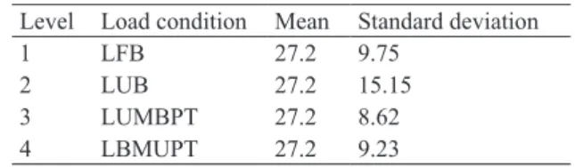
- For different load conditions their mean and standard deviation as taken as follows:
Level Load condition Mean Standard deviation
1 LFB 27.2 9.75
2 LUB 27.2 15.15
3 LUMBPT 27.2 8.62
4 LBMUPT 27.2 9.23
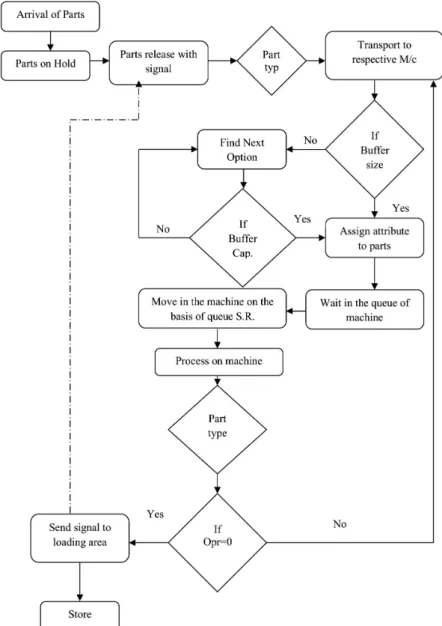
3.2. Modeling routing flexibility
The five different operations were considered for processing each part. The flexible system is considered four routing flexibility levels i.e. RF0, RF1, RF2 and RF3 under stochastic environment. RF=0, means that there is one to one relationship between machine and the part i.e. there is no alternative route for the parts. At RF=1, one operation can be done on two machines i.e. there is 1 more alternative machine for the same job (in addition to the machine available at RF=0). At RF=2, for one operation there are three alternative machines i.e. there is 2 more machines are available for processing the same operation in addition to the first one. Similarly for RF=3, 3 alternative machines
are available any part or operation as shown in the Figure 1. The makespan, resource utilization and work-in-process were considered as performance measures for processing 600 parts of 6 part types.
3.3. System capacity
The size of the input buffer of the machines represents the capacity of the manufacturing system. Four levels of the system capacity are considered in a way that, at an instant 30, 60, 90 and 120 parts present in system for processing.
3.4. System load conditions
The four system load conditions are taken in the proposed manufacturing model for the simulation i.e. Load Unbalanced (LUB), Load Full Balanced (LFB), Load Balanced Machine and Unbalanced Processing Time (LBMUPT) and Load Unbalanced Machine and Balanced Processing Time (LUMBPT).
In stochastic modeling the processing time may vary from one model to another with the influence of many factors, but in this paper it is assumed as
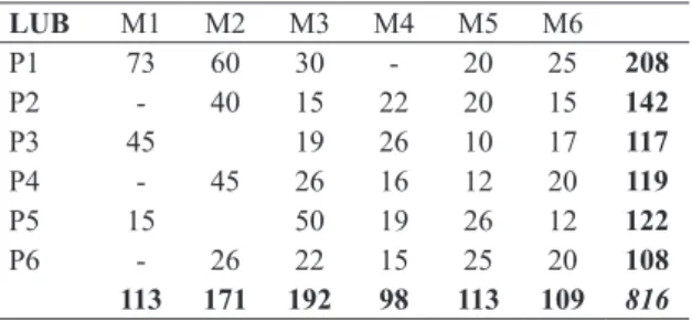
normally distributed. Ozcan et al. (2010) ignored the travel time in the calculation of total task time. They considered task times as normal distribution in stochastic environment. The operation times with the given load conditions are given in Tables 1–4. The mean and standard deviation of each load conditions are given along with the respected tables.
Table 1. System operating with LUB.
LUB M1 M2 M3 M4 M5 M6
P1 73 60 30 - 20 25 208
P2 - 40 15 22 20 15 142
P3 45 19 26 10 17 117
P4 - 45 26 16 12 20 119
P5 15 50 19 26 12 122
P6 - 26 22 15 25 20 108
113 171 192 98 113 109 816
Normal Distribution: Mean = 27.2, Stand. Deviation = 15.15
Table 2. System operating with LFB.
LFB M1 M2 M3 M4 M5 M6
P1 33 30 30 20 23 136
P2 40 20 32 25 19 136
P3 45 19 36 16 20 136
P4 40 25 30 25 16 136
P5 58 20 18 17 23 136
P6 26 22 20 33 35 136
136 136 136 136 136 136 816
Normal Distribution: Mean = 27.2, Stand. Deviation = 9.75
Table 3. System operating with LBMUPT.
LBMUPT M1 M2 M3 M4 M5 M6
P1 38 30 30 22 22 142
P2 35 20 32 23 20 130
P3 40 24 36 20 18 138
P4 37 20 30 21 18 126
P5 58 18 18 18 23 135
P6 34 24 20 32 35 145
136 136 136 136 136 136 816
Normal Distribution: Mean = 27.2, Stand. Deviation = 9.23
Table 4. System operating with LUMBPT.
LUMBPT M1 M2 M3 M4 M5 M6
P1 33 25 35 18 25 136
P2 35 25 32 20 24 136
P3 40 24 30 22 20 136
P4 38 27 25 31 15 136
P5 55 23 16 17 25 136
P6 25 20 20 35 36 136
128 123 154 123 143 145 816
Normal Distribution: Mean = 27.2, Stand. Deviation = 8.62
3.5. Sequencing rules
The sequencing rules are applied over the machine input buffer queue so that the parts are selected on account of the applicable sequencing rule (SR). The opted sequencing rules are:
- First-come-first-served (FCFS): Part that comes first in the machine buffer will be selected first for processing.
- Shortest processing time (SPT): Part having shortest processing time among parts present in the machine buffer will process first.
- Highest processing time (HPT): Part having highest processing time among parts present in the machine buffer will process first.
- Last-come-first-served (LCFS): Part that comes last in the machine buffer will be selected first for processing.
3.6. Performance measures
The model is evaluated by considering make-span time, resource utilization and work-in-process as the performance measures (Khan and Ali, 2015) are. Where:
Makespan time Cmax= max ij CTij
Resource utilization RU i SiUi/ Si
n
i n
1 1
=
|
=|
=Work-in-process (WIP) is referred to all parts and partly finished parts that are at different stages of the manufacturing process.
that machine and the required attributes are assigned. If number of parts in the machine buffer are equal to the capacity of the buffer then the part finds another route. Once all the buffers of the selected routes are full, the systems becomes blocked. The parts have to wait in machine buffer till machine completed its task. The next part moved into the machine for processing only when the in process part moved out from the machine. The next part enters on the bases of queue sequencing rules. Parts after being processed on a particular information is obtained to know whether all the operation of that part has been completed or not. If all the operations are completed, then the part is moved to the store. If any operation is left to perform then the part goes to the particular machine, where attributes are assigned.
Once all operations are completed for a part then it is sent for the storage. The information is sent in the form of a signal to loading station that releases same part type from the controlled input system provided in model. By this way, a constant volume is maintained in the manufacturing system. This process will go on till all the parts turned over through the system.
5. Experiment Design and
Methodology
Arena simulation software is used for the experimentation of proposed manufacturing model. A number of experiments have been performed to find out the effects of routing flexibility, system
capacity, system load condition and sequencing rule on the performance of the system. Make-span time, resource utilization and work-in-process are taken as the performance measure.
5.1. Assumptions of model
The aim of this work is to determine the effect of routing flexibility, system capacity, system load condition and sequencing rule on the performance of RFEMS under stochastic environment and to highlight the actual impact of these factors under different conditions. It is assumed that the processing time of the parts is considered as normally distributed with four different load conditions that are mentioned in the above section. The system capacity is controlled by maintaining the input buffer size of each machine. Sequencing rules are employed over each queue of the machine individually. The make-span time, resource utilization and work-in-process are considered as the performance measure. Each machine must process one part at an instance of time. Total processing time also include set-up times. Table 5 shows the four factors and their levels.
Table 5. Details of factor and their level.
S.No. Factor Factor level Level Id 1 Routing flexibility (RF) 0
1 2 3
1 2 3 4 2 System Capacity (SC) 30
60 90 120
1 2 3 4 3 System load (SL) LUB
LFB LUMBPT LBMUPT
1 2 3 4 4 Sequencing rules (SR) FCFS
SPT HPT LCFS
1 2 3 4
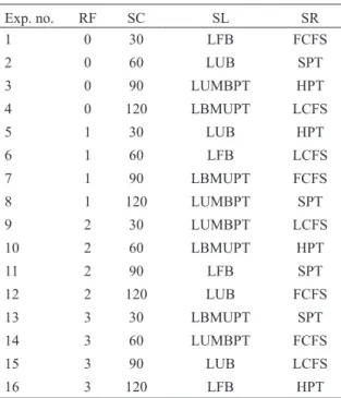
In the above designed conditions the total number of experiment required to perform the interactive study of the given factors and their levels are 256. Therefore, Taguchi’s concept of design of experiment is used to establish the best possible combinations of the given factors and their levels that drop the number of experiments to 16 shown in Table 6.
Table 6. Combination details of factors and levels.
Exp. no. RF SC SL SR
1 0 30 LFB FCFS
2 0 60 LUB SPT
3 0 90 LUMBPT HPT
4 0 120 LBMUPT LCFS
5 1 30 LUB HPT
6 1 60 LFB LCFS
7 1 90 LBMUPT FCFS
8 1 120 LUMBPT SPT
9 2 30 LUMBPT LCFS
10 2 60 LBMUPT HPT
11 2 90 LFB SPT
12 2 120 LUB FCFS
13 3 30 LBMUPT SPT
14 3 60 LUMBPT FCFS
15 3 90 LUB LCFS
16 3 120 LFB HPT
Phadke (1989) stated that for make-span time the natural scale is not appropriate because it gives negative calculation, which is meaningless. To avoid the negative prediction we may use well known decibel scale. So as to minimize the sensitivity of noise factor, we have to maximize α, as:
α= −10 log (make span)2
In regard to signal-to-noise (S/N) ratio, three types are described by Taguchi, i.e., smaller the-best, larger the-the-best, and nominal-the-best. For the analysis of results smaller-the-best is considered in case of make-span time and work-in-process, while for resource utilization, the larger-the-best was considered.
6. Experimental results
The proposed RFEMS model is simulated with the above consideration. The model is simulated for 600 parts of 6 part types. The results are presented in Table 7.
The ANOM is used to determine the optimal factor combinations for the designed RFEMS model, it may be defined as follows (Phadke 1989):
mjk = main factor effect for the kth level of factor j, i.e.:
ljki
t l
1
a
=
|
Where: j = the factor (i.e., routing flexibility, system capacity, system load condition, sequencing rules);
k = factor level (i.e., 1, 2, 3, or 4); αjki= the S/N ratio
of the factor j with level k; l = the time that factor j
with level k appears in the simulation model (i.e., 4).
6.1. Optimal factor combinations
According to the results getting from ANOM, the mjk
values for RFEMS with the three given performance measuring i.e. MST, WIP and RU are presented in Table 8. The S/N ratio for each of the optimal factor combination is signified by the maximum point on the graph as shown in the Figure 3, 4 and 5. Table 7. Orthogonal array L 16 (4) with experimental results and calculated S/N ratios.
Exp. No. RF SC SL SR MST/min. S/N ratio (dB) WIP (%) S/N ratio (dB) RU (%) RU ratio (dB)
1 1 1 1 1 31397 -89.93 45.59 -33.17 0.43 7.25
2 1 2 2 2 19761 -85.91 42.58 -32.58 0.69 3.16
3 1 3 3 3 18347 -85.27 43.26 -32.72 0.74 2.59
4 1 4 4 4 17596 -84.90 42.88 -32.64 0.77 2.22
5 2 1 2 3 31897 -90.07 44.52 -32.97 0.42 7.35
6 2 2 1 4 18606 -85.39 42.10 -32.48 0.73 2.70
7 2 3 4 1 15161 -83.61 40.78 -32.20 0.89 0.95
8 2 4 3 2 14142 -83.01 41.42 -32.34 0.96 0.33
9 3 1 3 4 32797 -90.31 43.46 -32.76 0.41 7.63
10 3 2 4 3 18910 -85.53 40.82 -32.21 0.71 2.87
11 3 3 1 2 14836 -83.42 40.44 -32.13 0.91 0.77
12 3 4 2 1 13903 -82.86 43.77 -32.82 0.98 0.14
13 4 1 4 2 32534 -90.24 42.96 -32.66 0.41 7.55
14 4 2 3 1 14795 -83.40 41.06 -32.26 0.91 0.74
15 4 3 2 4 14266 -83.08 42.41 -32.54 0.95 0.36
16 4 4 1 3 14258 -83.08 42.30 -32.52 0.95 0.41
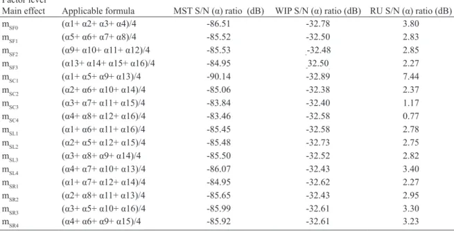
Table 8. Factor mean effects of matrix experiment Factor level
Main effect Applicable formula MST S/N (α) ratio (dB) WIP S/N (α) ratio (dB) RU S/N (α) ratio (dB)
mSF0 (α1+ α2+ α3+ α4)/4 -86.51 -32.78 3.80
mSF1 (α5+ α6+ α7+ α8)/4 -85.52 -32.50 2.83
mSF2 (α9+ α10+ α11+ α12)/4 -85.53 --32.48 2.85
mSF3 (α13+ α14+ α15+ α16)/4 -84.95 -32.50. 2.27
mSC1 (α1+ α5+ α9+ α13)/4 -90.14 -32.89 7.44
mSC2 (α2+ α6+ α10+ α14)/4 -85.06 -32.38 2.37
mSC3 (α3+ α7+ α11+ α15)/4 -83.84 -32.40 1.17
mSC4 (α4+ α8+ α12+ α16)/4 -83.46 -32.58 0.77
mSL1 (α1+ α6+ α11+ α16)/4 -85.45 -32.58 2.78
mSL2 (α2+ α5+ α12+ α15)/4 -85.48 -32.73 2.75
mSL3 (α3+ α8+ α9+ α14)/4 -85.50 -32.52 2.82
mSL4 (α4+ α7+ α10+ α13)/4 -86.07 -32.43 3.40
mSR1 (α1+ α7+ α12+ α14)/4 -84.95 -32.62 2.27
mSR2 (α2+ α8+ α11+ α13)/4 -85.65 -32.43 2.95
mSR3 (α3+ α5+ α10+ α16)/4 -85.99 -32.61 3.30
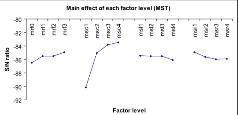
It is found in Figure 3 that the best factor level combination with MST is RF3, SC4, SL1 and SR1. Which shall be understood as the routing flexibility level 4, the system capacity 120, load fully balanced (LFB) and sequencing rule as FCFS.
It is also evident from the Figure 4 that the best factor level combination with WIP as performance measure is RF2, SC2, SL4 and SR2. This shall be easily read as the routing flexibility level 3, the system capacity 60, load balanced on machine and unbalanced processing time (LBMUPT) and sequencing rule as SPT.
It is shown in Figure 5 that the best factor level combination with RU is RF0, SC1, SL4 and SR3. This may be read as the routing flexibility level 1, the system capacity 30, load balanced on machine and unbalanced processing time (LUMBPT), and the sequencing rule is HPT.
It is also very important to discuss the relative significance of different factors on the system. For this analysis of variance (ANOVA) is implemented.
Main effect of each factor level (MST)
-92 -90 -88 -86 -84 -82 -80 m rf0 m rf1 m rf2 m rf3 m sc1 m sc2 m sc3 m
sc4 msl1 msl2 msl3 msl4 msr1
m sr2 m sr3 m sr4 Factor level S/N ra tio
Figure 3. Main effects of each factor level (MST).
Main effect of each factor level (WIP)
-33 -32.9 -32.8 -32.7 -32.6 -32.5 -32.4 -32.3 -32.2 -32.1 m rf0 m rf1 m rf2 m rf3 m sc1 m sc2 m sc3 m
sc4 msl1 msl2 msl3 msl4 msr1
m sr2 m sr3 m sr4 Factor level S/N ra tio
Figure 4. Main effects of each factor level (WIP).
Main effect of each factor level (RU)
0 2 4 6 8 m rf0 m rf1 m rf2 m rf3 m sc1 m sc2 m sc3 m
sc4 msl1 msl2 msl3 msl4 msr1
m sr 2 m sr 3 m sr 4 Factor level S/N ra tio
6.2. Analysis of variance
The significant factors can be found out by implementing analysis of variance (ANOVA). Where, the relative importances of factors are exposed by the error variance. The higher F-value means greater importance. Minitab statistical software is used to calculate the ANOVA at confidence level of 95%. The simulated results of the MST, WIP and RU of the system are taken from Table 8 for Preparation of the ANOVA table (Table 9). The importance of the factor is determined by the F-value Phadke (1989). From the Table 9 F-value of system capacity is maximum at MST and RU at the same time effect of routing flexibility is highest at WIP. But the sequencing rule is having the least effect at all performance measures.
7. Results and Discussions
Taguchi’s Design of Experiment (DOE) gives us a quick means to find out the behavior of different factors in a Manufacturing System. It is established from the above analysis the best factors and their levels combination with make-span time is RF3, SC4, SL1 and SR1, that may read as the routing
flexibility level 4, system capacity 120, Load unbalanced (LUB), and the sequencing rule as FCFS where as for resource utilization the best combination is RF0, SC1, SL4 and SR3, whereas RF2, SC2, SL4 and SR2 is the best combination for work-in-process measurement. In light of results obtained each of factor is discussed briefly in the following sections.
7.1. Routing flexibility
It is seen in Figure 3 that there is a major effect of routing flexibility with the make-span time on the performance of RFEMS. It decreases with the increase in the level of routing flexibility. At RF=0 the parts moved through fixed route. Routing flexibility is exploited as RF level increases, in result there is decrease in MST. Figure 4 shows that as the routing flexibility increases the WIP reduce. This phenomenon happens up to RF2 and then there is a slight increase at RF3. WIP is maximum at RF=0, as the parts wait in machine buffers for processing, in so doing increasing the WIP. It is also view from Figure 5 that the RU reduces with the increase in RF level. This is because at lower levels of RF the parts are processed through a fixed route resulting decrease in RU. It is also observed from Tablex9 that
Table 9. ANOVA results showing at different outputs (RF).
ANOVA for Means (MST)
Source DF Seq SS Adj SS Adj MS F P
RF 3 16320178 16320178 5440059 4.28 0.132 SC 3 782739183 782739183 260913061 205.32 0.001
SL 3 3983854 3983854 1327951 1.05 0.486
SR 3 10964563 10964563 3654854 2.88 0.204 Residual Error 3 3812234 3812234 1270745
Total 15 817820013
ANOVA for Means (WIP)
Source DF Seq SS Adj SS Adj MS F P
RF 3 5.9762 5.9762 1.9921 3.74 0.154 SC 3 16.0854 16.0854 5.3618 10.06 0.045 SL 3 4.5263 4.5263 1.5088 2.83 0.208 SR 3 2.4233 2.4233 0.8078 1.52 0.370 Residual Error 3 1.5983 1.5983 0.5328
Total 15 30.6095
ANOVA for Means (RU)
Source DF Seq SS Adj SS Adj MS F P
RF 3 0.046771 0.046771 0.015590 8.19 0.059 SC 3 0.602995 0.602995 0.200998 105.56 0.002 SL 3 0.010807 0.010807 0.003602 1.89 0.307 SR 3 0.023346 0.023346 0.007782 4.09 0.139 Residual Error 3 0.005712 0.005712 0.001904
impact of routing flexibility is highest when RU is taken as performance measure and followed by MST and WIP.
7.2. System capacity
It is evident from the Figure 3 that there is a remarkable improvement in the MST of the proposed RFEMS. MST decreases with increase in system capacity. Increase in the system capacity means more parts are permissible to move in the system resulting better load sharing so as MST is reduced. Figure 4, shows that the WIP is significantly reduced from SC1 to SC2 and then there is a marginal increase with the increase in system capacity level. It is also found from Figure 5 that the average resource utilization increases with the increase in the capacity of the system. It is because at higher levels of SC resources constantly in working therefore RU increases. From the results Table 9 shows system capacity effect most at MST and followed by RU and WIP.
7.3. System load condition
Figure 3 show that, the RFEMS perform in a different way with different system load conditions with make-span time. It is maximum at LBMUPT and minimum at LFB. From Figure 4, it is clear that WIP is maximum with LUB and minimum with LBMUPT system load condition. It is evident from Figure 5, that RU is highest when LBMUPT is taken and it is lowest when LUB is takes as system load condition. This is so because when the model is simulated with LUB then there is maximum load sharing on the machines therefore average resource utilization increases. It is also observed from Table 9 that the effect of SL is significant by considering WIP and then followed by RU and MST as performance measure.
7.4. Sequencing rules
Sequencing rules have a little impact on the MST and RU performance of RFEMS as shown in Figure 3 and 5. They are minimum when FCFS is taken into consideration. While Figure 4 shows the minimum WIP at SPT. It is also observed from Table 9 that effect of sequencing rule is most dominating by considering RU as performance measure and then MST and WIP.
8. Conclusions
In this paper, discrete-event simulation model is used to analyze the impact of some factors i.e. routing flexibility, system capacity, system load condition and sequencing rule on the performance of a RFEMS. For experiment design Taguchi’s DOE framework is used and the results are analyzed statically. It is found that increase in the routing flexibility level is not the only means for the system performance improvement. By using the proposed model, the best possible levels of some other factors are also considered, i.e. system capacity, system load condition, and sequencing rule. In spite of whole of this study, there are some limitations exist that may be explored further. One of the key limitation of this study is the model cannot be used for all manufacturing domain. An extensive data set may be modeled for getting better results. The focus of this work is for the development of a demonstrative platform to show major areas of concern and key directions. Keeping these limitations in mind future work can be undertaken by considering other flexibility types, number of machines, parts, operations, etc.
References
Ali, M., Wadhwa, S. (2010). The Effect of Routing Flexibility on a flexible system of Integrated Manufacturing. International Journal of Production Research, 48(19), 5691-5709. https://doi.org/10.1080/00207540903100044
Barad, M., Sapir, D. E. (2003). Flexibility in Logistic Systems-Modeling and Performance Evaluation. International Journal of Production Economics, 85, 155-170. https://doi.org/10.1016/S0925-5273(03)00107-5
Blackburn, J., Millen R. (1986). Perspectives on Flexibility in Manufacturing: Hardware versus Software, In Andrew R. Rachamadugu and T.J. Schriber Kusiak Modeling and Design of Flexible Manufacturing Systems, 2, 2, , Ed. Elsevier Science Publishers, Amsterdam, The Netherlands, 116-117.
Browne J., Dubois, D., Rathmill, K., Seth, S. P., Stecke, K. E. (1984). Classification of Flexible Manufacturing Systems. The FMS Magazine 114.
Gerwin, D. (1993). Manufacturing Flexibility: A Strategic Perspective. International Journal of Management Science, 39(4), 395-410. https://doi.org/10.1287/mnsc.39.4.395
Gustavsson, S. O. (1984). Flexibility and Productivity in Complex Production Processes. International Journal of Production Research, 22, 801-808. https://doi.org/10.1080/00207548408942500
Joseph, O. A., Sridharan, R. (2012). Effect of Flexibility and Scheduling decisions the Performance of an FMS: Simulation modeling and analysis. International Journal of Production Research, 50(7), 2058-2078. https://doi.org/10.1080/00207543.2011.575091 Khan W. U., Ali. M. (2015), Effect of Sequencing Flexibility on the performance of Flexibility Enabled Manufacturing System. International
Journal of Industrial and Systems Engineering, 21(4), 474-498. https://doi.org/10.1504/IJISE.2015.072731
Mehdi S., Zaki S., Ahmed, H. (2013). Real-time rescheduling metaheuristic algorithms applied to FMS with routing flexibility. International Journal of Advanced Manufacturing Technology, 64(1-4), 145. https://doi.org/10.1007/s00170-012-4001-y
Ozcan U., Kellegoz, T., Toklu, B. (2010). A genetic algorithm for the stochastic mixed-model U-line balancing and sequencing problem. International Journal of Production Research, 49(6), 1605-1626, https://doi.org/10.1080/00207541003690090
Pankaj, C., Mihkel, M. T. (1991). Models for the Evaluation of Routing and Machine Flexibility. European Journal of Operational Research, 60(2), 156-165. https://doi.org/10.1016/0377-2217(92)90090-V
Phadke, M. S. (1989). Quality engineering robust design. Englewood Cliffs, NJ: Prentice-Hall.
Rohit P., Nishant S., Arvind S. T. (2016). Performance Evaluation of Flexible Manufacturing System (FMS) in Manufacturing Industries. Imperial Journal of Interdisciplinary Research, 2(3), 2454-1362
Savsar, M., Aldaihani, M. (2012). A Stochastic Model for Analysis of Manufacturing Modules. Applied Mathematics and Information Science 6(3), 587-600.
Sethi, A. K., Sethi, S. P. (1990). Flexibility in Manufacturing: A Survey. International Journal of Flexible Manufacturing Systems, 2, 289-328. https://doi.org/10.1007/BF00186471
Wadhwa, S., Bhagwat, R. (1998). Judicious Increase in Flexibility and Decision Automation in Semi-Computerized Flexible Manufacturing (SCFM) Systems. International Journal, Studies in Informatics and Control, 2(8), 329-342.
Wadhwa, S., Ducq, Y., Mohammed, A., Prakash, A. (2008). Performance Analysis of a Flexible Manufacturing System under Planning and Control Strategies. International Journal, Studies in Informatics and Control, 17(3), 273-284.
Wahab, M. I. M. (2005). Measuring machine and product mix flexibilities of a manufacturing system. International Journal of Production Research, 43(18), 3773-3786. https://doi.org/10.1080/00207540500147091