SOME CONTRIBUTIONS TO DATA DRIVEN INDIVIDUALIZED DECISION MAKING PROBLEMS
Zhengling Qi
A dissertation submitted to the faculty of the University of North Carolina at Chapel Hill in partial fulfillment of the requirements for the degree of Doctor of Philosophy in the
Department of Statistics and Operations Research.
Chapel Hill 2019
c ⃝2019 Zhengling Qi
ABSTRACT
ZHENGLING Qi: SOME CONTRIBUTIONS TO DATA DRIVEN INDIVIDUALIZED DECISION MAKING PROBLEMS
(Under the direction of Yufeng Liu)
Recent exploration of the optimal individualized decision rule (IDR) for patients in preci-sion medicine has attracted a lot of attentions due to the potential heterogeneous response of patients to different treatments. In the current literature, an optimal IDR is a decision function based on patients’ characteristics for the treatment that maximizes the expected outcome. My dissertation research mainly focuses on how to estimate optimal IDRs under various criteria given experimental data.
To my parents, Jianxin Qi and Zhi Zheng,
and my beloved wife, Xutong Zhao,
ACKNOWLEDGEMENTS
I feel so grateful and fortune that I have had the opportunity over the past four years working on exciting and challenging statistical problems, and turning them into my Ph.D. dissertation. It is one of the most enjoyable and fulfilling Ph.D. experiences that anybody could hope for. I could not imagine having better support from my advisor, committee members, colleagues, friends and family.
First of all, I would like to express my deepest gratitude to my advisor Dr. Yufeng Liu for his tremendous help of my Ph.D. study and related research, for his patience, encouraging and motivation. He has taught me how to start doing research, to learn and think with his rich knowledge and extensive experience. His technical and editorial advice was essential to the completion of this dissertation. Besides research, he has many impressive traits that I hope to cultivate. He inspires me for the value of seeking simplest but most useful solutions and persisting on them. He shows me how to be an amazing mentor to students that I hope I could be. Your advice on both research as well as my career has been invaluable.
I would also like to thank my committee members: Dr. Shu Lu, Dr. J.S. Marron, Dr. Jong-Shi Pang and Dr. Donglin Zeng, who provide me insightful suggestions on my dissertation. Those invaluable comments have greatly improved this dissertation. I am also grateful to Dr. Edward Carlstein, who has given me a lot of great comments and suggestions during my job search.
I also want to thank Dr. Ji Zhu for his kind support during my master study at University of Michigan, Ann Arbor. Without his encouragement, I would not pursue a Ph.D. and have the chance to enjoy the beauty of doing research in statistics.
I am also thankful to all my fellow colleagues, especially those lovely basement friends. Special appreciation goes to Wawa, Small little face, ZZQ, Tony Fan, Jonathan P Williams, Iain Carmichael and all the members in Dr. Yufeng Liu’s research group.
I am very grateful to all my friends, who always support me through my Ph.D. study. Special appreciation alphabetically goes to Yifan Cui, Ying Cui, Ruituo Fan, Cui Guo, Peng Liao, Xia Lu, Hongsheng Liu, Wenbo Sun, Lu Tang, Nalingna Yuan, Ruofei Zhao and Jinyang Zheng.
TABLE OF CONTENTS
LIST OF TABLES . . . x
LIST OF FIGURES . . . xiii
LIST OF ABBREVIATIONS AND SYMBOLS . . . xiv
1 Introduction . . . 1
1.1 Multi-armed Angle-based Direct Learning for Estimating Optimal In-dividualized Decision Rules with Various Outcomes . . . 1
1.2 Estimating Individualized Decision Rules with Tail Controls . . . 1
1.3 Estimation of Individualized Decision Rules Based on an Optimized Covariate-Dependent Equivalent of Random Outcomes . . . 2
2 Multi-armed Angle-based Direct Learning for Estimating Optimal Individu-alized Decision Rules with Various Outcomes . . . 4
2.1 Introduction . . . 4
2.2 Angle Based Direct Learning . . . 7
2.2.1 The Direct Learning Framework . . . 8
2.2.2 Angle Based D-learning for Continuous Outcomes . . . 10
2.2.3 Estimation Procedures of AD-learning . . . 13
2.3 Extensions to Other Types of Outcomes . . . 16
2.3.1 Binary Outcomes . . . 16
2.3.2 Survival Outcomes . . . 17
2.4 Theoretical Properties of AD-learning . . . 19
2.5 Simulation Study . . . 22
2.5.1 Study of Continuous Outcomes . . . 23
2.5.2 Study of Binary and Survival Outcomes . . . 25
2.6 Real Data Applications . . . 28
2.7 Conclusion . . . 31
3 Estimating Individualized Decision Rules with Tail Controls . . . 32
3.1 Introduction . . . 32
3.2 Robust Criteria to Estimate Optimal IDRs . . . 35
3.2.1 Expected Value Function Framework . . . 35
3.2.2 Conditional Value at Risk . . . 36
3.2.3 Robust Criteria for IDR Problems . . . 38
3.2.3.1 Average Lower Tail . . . 38
3.2.3.2 Individualized Lower Tails . . . 39
3.2.4 Duality Representation . . . 41
3.3 Statistical Estimation and Optimization . . . 44
3.3.1 Estimation of Optimal IDRs underM1(d) . . . 45
3.3.2 Estimation of Optimal IDRs underM2(d) . . . 49
3.4 Theoretical Results . . . 51
3.4.1 Fisher Consistency . . . 52
3.4.2 Excess Value Bound . . . 52
3.4.3 Convergence Rate . . . 52
3.5 Simulation Studies . . . 55
3.5.1 A Motivating Example Revisit . . . 56
3.5.2 Distributional Shift Examples . . . 58
3.5.3 Simulation Scenarios . . . 59
3.6 Real Data Applications . . . 62
3.7 Conclusion . . . 64
4 Estimation of Individualized Decision Rules Based on An Optimized Covariate-dependent Equivalent of Random Outcomes . . . 66
4.1 Introduction . . . 66
4.1.2 Optimized certainty equivalent . . . 68
4.1.3 Contributions and organization . . . 70
4.2 The IDR-based CDE . . . 71
4.2.1 Definition and properties . . . 71
4.2.2 The IDR optimization problem . . . 76
4.2.3 Decomposable space and normal integrand . . . 77
4.2.4 Illustrative examples . . . 79
4.3 The Empirical IDR Optimization Problem . . . 83
4.4 Solving a Piecewise Affine Constrained DC Program . . . 88
4.5 Numerical Experiments . . . 96
APPENDIX A SUPPLEMENTARY MATERIAL TO CHAPTER 2 . . . 101
APPENDIX B SUPPLEMENTARY MATERIAL TO CHAPTER 3 . . . 115
LIST OF TABLES
2.1 Results of average means (standard deviations) of empirical value func-tions and misclassification rates for four continuous-outcome simulation scenarios with 40 covariates. The best value functions and
misclassifi-cation rates are in bold. . . 25 2.2 Results of average means (standard deviations) of empirical value
func-tions and misclassification rates for two binary-outcome simulation sce-narios with 40 covariates. The best value functions and misclassification
rates are in bold. . . 26 2.3 Results of average means (standard deviations) of empirical value
func-tions and misclassification rates for two survival-outcome simulation scenarios with 40 covariates. The best value functions and
misclassifi-cation rates are in bold. . . 27 2.4 Results of average means (standard deviations) of empirical value
func-tions and misclassification rates for six high dimensional simulation
scenarios. The best value functions and misclassification rates are in bold. . . 28 2.5 Results of coefficients estimation for comparison functions. . . 29 2.6 Results of empirical value functions on one fold of testing data. The
best empirical value function is in bold. . . 30 2.7 Results of coefficient estimation for survival time of failure. . . 31
3.1 Comparisons of misclassification error rates (standard error) for
simu-lated examples with n= 200 andp= 20. . . 59 3.2 Comparisons of misclassification error rates (standard deviation) for
simulated examples with n= 200 andp = 20. From left to right, each column represents Scenarios (1)-(8) respectively. Each row represents one specific method. The last six rows correspond to our proposed
methods. . . 61 3.3 Comparisons of average value functions (standard deviation) for
sim-ulated examples with n = 200 and p = 20. From left to right, each column represents scenarios (1)-(8) respectively. Each row represents one specific method. The last six rows correspond to our proposed
methods. . . 61 3.4 Comparisons of 50% quantiles (standard deviation) of value functions
for simulated examples with n= 200 and p = 20. From left to right, each column represents scenarios (1)-(8) respectively. Each row repre-sents one specific method. The last six rows correspond to our proposed
3.5 Comparisons of 25% quantiles (standard deviation) of value functions for simulated examples with n= 200 and p = 20. From left to right, each column represents scenarios (1)-(8) respectively. Each row repre-sents one specific method. The last six rows correspond to our proposed
methods. . . 62 3.6 Results of Value function comparison. First column represents the
means of empirical value functions. Second and third columns rep-resent means of 50% and 25% quantiles of empirical value functions,
respectively. . . 64
4.1 The average computational times (in seconds) and dc iteration numbers forp= 10.. . . 98 4.2 Average misclassification rates (standard errors) and average means (standard
errors) of empirical value functions for three simulation scenarios over 100 runs. The best expected value functions and the minimum misclassification rates are
in bold. . . 99 4.3 Results of average 25% (standard errors) and 50% (standard errors) quantiles
of empirical value functions for three simulation scenarios over 100 runs. The
largest 25% and 50% quantiles are in bold. . . 100
A.1 Results of average means (standard deviations) of empirical value func-tions and misclassification rates for four continuous-outcome simula-tions scenarios with 20 covariates. The best value funcsimula-tions and
mis-classification rates are in bold. . . 107 A.2 Results of average means (std) of empirical value functions and
misclas-sification rates for four continuous-outcome simulation scenarios with n = 200. The best value functions and misclassification rates are in
bold. . . 108 A.3 Results of average means (standard deviations) of empirical value
func-tions and misclassification rates for two binary-outcome simulation sce-narios with 20 covariates. The best value functions and misclassification
rates are in bold. . . 109 A.4 Results of average means (standard deviation) of empirical value
func-tions and misclassification rates for two binary-outcome simulation sce-narios with n = 200. The best value functions and misclassification
rates are in bold. . . 109 A.5 Results of average means (standard deviations) of empirical value
func-tions and misclassification rates for two survival-outcome simulation scenarios with 20 covariates. The best value functions and
A.6 Results of average means (standard deviation) of empirical value func-tions and misclassification rates for two survival-outcome simulation scenarios with n= 200. The best value functions and misclassification
rates are in bold. . . 110 A.7 Results of average means (std) of empirical value functions and
misclas-sification rates for four continuous-outcome simulation scenarios with
20 covariates. The best value functions and misclassification rates are in bold. . . . 112 A.8 Results of average means (std) of empirical value functions and
misclas-sification rates for four continuous-outcome simulation scenarios with
40 covariates. The best value functions and misclassification rates are in bold. . . . 113 A.9 Results of average means (std) of empirical value functions and
mis-classification rates for two simulation scenarios with 20 covariates. The
best value functions and misclassification rates are in bold. . . 113 A.10 Results of average means (std) of empirical value functions and
misclas-sification rates for one continuous-outcome simulation scenarios with 20 covariates. The best value functions and misclassification rates are in
LIST OF FIGURES
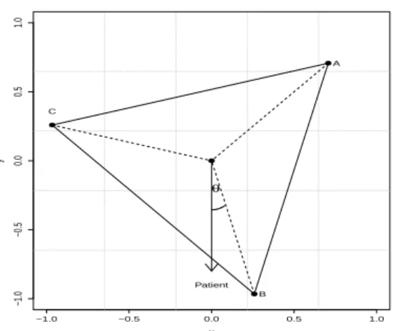
2.1 Graphical illustration of the estimated IDR for a given patient in a three-treatment setting. Vertices A, B and C represent 3 treatments. The estimated IDR of the patient has the least angle with treatmentB
which is thus more preferable than the other two treatments. . . 6 2.2 Geometric interpretation of our least angle decision rule. When K = 3
orK= 4, the estimate ˆf has the smallest angle with treatment 1 so we recommend treatment 1 as the optimal treatment. When K = 2, we can see ˆf has the smallest angle with vector w2 and the optimal rule
for this patient is treatment 2. . . 12
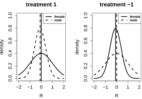
3.1 Plots of a motivating example. The dash and solid lines in the left plot show the probability densities of N(-0.1,0.5) andN(0,1) respectively. The dash and solid lines in the right plot correspond to the probability densities ofN(0,1) andN(-0.1,0.5) respectively. In this example, male is more preferable to treatment 1, while female is more preferable to
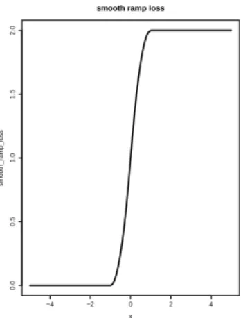
treatment -1. . . 33 3.2 Plot of smooth surrogate loss function with δ= 1 . . . 46 3.3 Box plots of value functions computed by three methods. The left
box plot corresponds to the result of l1-PLS under the expected-value
function framework. The middle and the right box plots correspond to
the result of our proposed methods under M1(d) andM2(d) respectively. . . 57
3.4 Medians and standard deviations of value functions under different com-binations of τ and γ by l2-DC-CVaR. The left plot corresponds to the
medians and the right plot corresponds to the standard deviations of
value functions respectively. . . 58
LIST OF ABBREVIATIONS AND SYMBOLS IDR
AD-learning OCE
CDE CVaR DC MM D-learning l1-PLS
OWL RWL CPH DL ACWL VT DCA VaR
Individualized Decision Rules Angle-based direct learning Optimized Certainty Equivalent Covariates dependent equivalent Conditional Value at Risk Difference-of-convex Majorization-minimization Direct learning
l1 penalized least square
Outcome weighted learning Residual weighted learning Cox Proportional Hazard Decision list
Adaptive contrast weighted learning Virtual twins
CHAPTER 1 Introduction
In this chapter, we outline the contributions in the subsequent development of the disser-tation.
1.1 Multi-armed Angle-based Direct Learning for Estimating Optimal Individu-alized Decision Rules with Various Outcomes
Estimating an optimal individualized decision rule (IDR) based on patients’ information is an important problem in precision medicine. An optimal IDR is a decision function that optimizes patients’ expected clinical outcomes. Many existing methods in the literature are designed for binary treatment settings with the interest of a continuous outcome. Much less work has been done on estimating optimal IDRs in multiple treatment settings with good interpretations. In this paper, we propose an angle-based direct learning (AD-learning) method to efficiently estimate optimal IDRs with multiple treatments. Our proposed method can be applied to high dimensional settings under various types of outcomes, such as continuous, survival or binary outcomes. Moreover, it has an interesting geometric interpretation on the effect of different treatments for each individual patient, which can help doctors and patients make better decisions. Finite sample error bounds have been established to provide a theoretical guarantee for AD-learning. Finally, we demonstrate the superior performance of our method via extensive simulation studies and real data applications.
1.2 Estimating Individualized Decision Rules with Tail Controls
dissertation, we propose two new robust criteria to estimate optimal IDRs: one is to control the average lower tail of the subjects’ outcomes and the other is to control the individualized lower tail of each subject’s outcome. In addition to optimizing the individualized expected outcome, our proposed criteria take risks into consideration, and thus the resulting IDRs can prevent adverse events caused by the heavy lower tail of the outcome distribution. Interestingly, from the perspective of duality theory, the optimal IDR under our criteria can be interpreted as the decision rule that maximizes the “worst-case” scenario of the individualized outcome within a probability constrained set. The corresponding estimating procedures are implemented using two proposed efficient non-convex optimization algorithms, which are based on the recent de-velopments of difference-of-convex (DC) and majorization-minimization (MM) algorithms. We provide a comprehensive statistical analysis for our estimated optimal IDRs under the proposed criteria such as consistency and finite sample error bounds. Simulation studies and a real data application are used to further demonstrate the robust performance of our methods.
1.3 Estimation of Individualized Decision Rules Based on an Optimized Covariate-Dependent Equivalent of Random Outcomes
CHAPTER 2
Multi-armed Angle-based Direct Learning for Estimating Optimal Individualized Decision Rules with Various Outcomes
2.1 Introduction
Precision medicine, which recommends different treatments for individual patients, has been a popular research area in the scientific community. Compared with traditional “one-size-fits-all” medical procedures, precision medicine provides an individualized decision for each patient based on their information, such as clinical covariates, genetics, in order to maximize the outcome of each patient. In practice, there exists various types of outcomes such as time to event, health index or the disease indicator.
Censored data are commonly seen in practice because of early drop out or other reasons. Thus, it is also important to develop methods to estimate optimal IDRs for the survival outcome. Various methods have been proposed in the literature to estimate optimal IDRs for survival outcomes, such as (Goldberg and Kosorok, 2012; Zhao et al., 2015b) and (Cui et al., 2017). Recently, (Bai et al., 2016) and (Jiang et al., 2016) proposed several methods to estimate the optimal IDR that can maximize the survival probability of patients.
In the current literature, most of these existing methods are designed for binary treatment settings only. But there are many multi-armed IDR problems in pratice ((Baron et al., 2013)). To the best of our knowledge, not much has been done for estimating the optimal IDR for the multi-armed treatment settings with various outcomes, such binary and survival outcomes. Thus it is essential to develop methods to take multiple treatments into consideration simul-taneously and estimate optimal IDRs for various outcomes, which can help to improve the estimating efficiency and the classification accuracy.
−1.0 −0.5 0.0 0.5 1.0
−1.0
−0.5
0.0
0.5
1.0
x
y
Patient
θ
A
B C
Figure 2.1: Graphical illustration of the estimated IDR for a given patient in a three-treatment setting. VerticesA, BandC represent 3 treatments. The estimated IDR of the patient has the least angle with treatmentB which is thus more preferable than the other two treatments.
To get accurate estimation of optimal IDRs and obtain a good interpretation jointly under the multi-armed setting, we consider aK-vertex simplex structure in an Euclidean space, where each vertex represents one treatment. The simplex lies in a K-1 dimensional space with the origin as the center and has equal inner products among vertices. Using the expression of the optimal IDR, we transform the problem of maximizing the value function into maximizing the inner product between the decision function vector and the corresponding vertex in the simplex space. Such a transformation allows us to estimate the optimal IDR using multiple response regression methods. In particular, for each patient, our estimated decision function vector maps the covariates into thisK−1 dimensional space. The angle between each treatment vertex and the estimation function vector can be interpreted as a measure of preference to this treatment. We recommend a patient to take the corresponding treatment having the least angle with our estimated decision function vector. Figure 2.1 shows an example with our estimated IDR for a given patient. In this case, we recommend treatment B as the best option for this patient. In addition, we can see treatment C is more preferable than treatment A for this patient based on their corresponding angles.
such as binary and survival responses. Compared with existing methods, our proposed AD-learning enjoys several advantages. In particular, our method is robust in the sense that it is not necessary to model the main effect function of the conditional outcome. Due to direct learning scheme, our method does not suffer from the mismatch problem between minimizing prediction errors and maximizing value functions in model based methods such asl1-PLS ((Qian and
Mur-phy, 2011)) and can perform better in high dimensional settings. Moreover, by representing each treatment as a vertex of a standard simplex in the Euclidean space, our proposed method provides an attractive geometric interpretation of the relative effectiveness of all treatments for a given patient. The resulting relative effectiveness of different treatments can be interpreted as the angles between the decision function vector for the patient and each vertex corresponding to the treatment. These angles can be scaled between [0, π]. In addition, flexible structures such as group and low rank sparsity can be also incorporated to further improve the model interpretation and simplicity, which can be applied in high dimensional settings. Finally, our proposed method is easy to implement with efficient algorithms.
The remainder of Chapter 2 is organized as follows. In Section 2.2, we introduce our AD-learning to estimate optimal IDRs in multiple treatment settings. In Section 2.3, we discuss how to extend our proposed method to binary and survival outcomes. In Section 2.4, we provide a theoretical guarantee for our AD-learning under some mild assumptions. In Section 2.5, we conduct an extensive simulation study to evaluate the finite sample performance of our method with implementation details including algorithms. Furthermore, we illustrate our method using the AIDS data in Section 2.6. We conclude our paper with some discussions and possible future extensions in Section 2.7. Details of proof and additional simulation results are given in the Appendix A.
2.2 Angle Based Direct Learning
For notation of this Chapter, we use boldface capital and lowercase symbols to denote matrices and vectors respectively. For a matrixB, we define a mixedl1andl2norm as||B||2,1=
∑
||Bj||2, whereBjis thej-th row vector ofB. We use Tr(B) to denote the sum of the diagonal
We consider a randomized treatment framework for estimating optimal IDRs. For each patient, we observe a triplet random vector (x, A, R). In particular, x= (1, X1,· · · , Xp) ∈ X
denotes patients’p-dimensional covariates with an intercept. The random variableArepresents the randomized treatment that a patient receives. Here we consider the K-treatment-armed setting where A∈ {1,2,· · ·, K} with a known prior probability distribution π(A,x), which is the conditional probability depending on x. In a general setting other than the randomized trial study, π(A,x) denotes the propensity score and can be estimated by the generalized linear models such as multinomial logistic regression. The variable R is a patient’s outcome after receiving the treatment A. Without loss of generality, we assume that the outcome R is bounded and the largerR is, the better the treatment works for this patient.
One of the most important goals of our problem is to estimate the optimal IDR that can maximize the expected clinical outcome of each patient under this IDR. Mathematically speaking, an IDR is a decision function d(x) :X → A, mapping from the covariate space into the treatment space. According to (Qian and Murphy, 2011) and (Zhao et al., 2012), the value function under the IDR dcan be expressed as
V(d) =:E[R|d(x) =A] =E[RI(A=d(x)
π(A,x) ], (2.1)
whereI(•) is the indicator function. Then the optimal IDR is defined as
d0(x) = argmaxd∈DV(d) (2.2)
within a pre-specified class of treatment rulesD. Before introducing our proposed AD-learning, we first discuss the direct learning framework.
2.2.1 The Direct Learning Framework
represent the optimal IDR as
d0(x) = sign(E[R|x, A= 1]−E[R|x, A=−1])
= sign(E[ RA
π(A|x)|x]) := sign(f0(x)).
(2.3)
Using Equation (2.3), similarly in (Tian et al., 2014), the IDR problem is equivalent to estimate the optimal decision function f0(x) = E[π(ARA|x)|x] via various regression methods such as l1
penalized regression (LASSO). The final decision rule is determined by the sign of this estimator. Binary D-learning directly estimates the decision rule. It is very different from the out-come weighted learning (OWL) proposed by (Zhao et al., 2012) because binary D-learning uses regression methods to estimate the optimal IDR directly. Note that binary D-learning can be simply extended to theK-treatment-arm setting by rewriting the optimal IDR as
d0(x) = argmax k∈{1,···,K}
E[R|x, A=k]
= argmax
k∈{1,···,K}
KE[R|x, A=k]−
K
∑
i=1
E[R|x, A=i]
= argmax
k∈{1,···,K} K
∑
i̸=k
{E[R|x, A=k]−E[R|xA=i]}
= argmax
k∈{1,···,K} K
∑
i̸=k
E[ RAki πki(Aki,x)|
x, A=kori]
:= argmax
k∈{1,···,K} K
∑
i̸=k
fki(x) := argmax k∈{1,···,K}
fk(x),
(2.4)
whereAki∈ {−1,1}represents treatmentskandi, andfki(x) is defined as the optimal decision
function between treatment k and i. Each pairwise decision function can be estimated by a binary D-learning method. The final treatment decision rule is to compare the cumulative sum of pairwise decison functions fk(x) fork= 1,· · · , K, and select the largest one. We refer this
pairwise method as pairwise D-learning.
measure fk(x) can capture the relative strength of a treatment for a given patient, it may be
suboptimal.
To handle multi-armed IDR problems, we propose AD-learning that considers all treatments together to estimate the optimal IDR. Moreover, the AD-learning can provide a more effective measure of treatments for patients with a good interpretation.
2.2.2 Angle Based D-learning for Continuous Outcomes
For a K-armed IDR problem, one natural approach is to estimate K functions for all treatments. Since only one function is needed for the binary IDR problem, one indeed only needs K−1 functions for a K-armed problem. Instead of using K functions with a constraint on these functions, we aim to directly estimate K −1 functions. To that end, we project the treatment A into K simplex vertices defined on RK−1. Specifically, we encode the j-th treatment as a vector wj ∈ RK−1 with
wj =
(K−1)−1/21K−1, ifA= 1
−(1 +√K)/(K−1)3/21K−1+ (KK−1)1/2eA−1, if 2≤A≤K,
(2.5)
where ei is a K −1 dimensional vector with every element being 0, except the i-th location
being 1. Definewas a random vector withP[w=wj|x] =P[A=j|x]. This simplex encoding
scheme has several properties. In particular, the center of these vertices is the origin of the space, that is ∑Kj=1wj = 0 with ||wj||2 = 1 for j = 1,· · · , K. The angle between each pair of
K. Interestingly, we can then express the optimal IDR as
d0(x) = argmax k∈{1,···,K}
E[R|x, A=k] = argmax
k∈{1,···,K}
(1−c(K))E[R|x, A=k]
= argmax
k∈{1,···,K}
{(1−c(K))E[R|x, A=k] +c(K)
K
∑
j=1
E[R|x, A=j]}
= argmax
k∈{1,···,K}
{E[R|x, A=k] +c(K)
K
∑
j̸=k
E[R|x, A=j]}
= argmax
k∈{1,···,K}
{wTkE[Rw|x, A=k] +wTk
K
∑
j̸=k
E[Rw|x, A=j]}
= argmax
k∈{1,···,K}
wTkE[ Rw
π(A,x)|x] := argmaxk∈{1,···,K}w
T kf0(x),
(2.6)
where f0(x) is a function vector from Rp+1 to RK−1 with some abuse of notation. Then the
optimal IDR is given by comparing the inner product betweenwkand f0(x) for each treatment
k. We define the angle between each pair of vertices in [0, π]. Then wTkf0(x) is the largest if
and only if the angle between wk and f0(x) is the least, for k = 1,· · · , K. Thus we call our
proposed method as Angle based D-learning (AD-learning). Note that the simplex coding is unique up to the orthogonal rotation.
Our proposed AD-learning has an attractive geometric interpretation. In particular, this least angle decision rule can be understood through newly defined treatment regions for each patient. For example, when K = 3, as shown in Figure 2.2 (b), vectors wk; k = 1,· · · , K
form an equilateral triangle in the R2 space, where each divided region represents a treatment region. The decision function vector f0(x) maps from the covariate space into the treatment
region. One can observe that the angles between vertices are the same, and consequently each treatment is treated equally. Such a simplex coding scheme does not require a balanced group size for each treatment since treatment proportions are taken into account by the termπ(A,x) in Equation (2.6). We name the angle between eachwk andf0(x) as thetreatment score which
w2=−1 O= 0 w1= 1 ˆ
f
(a)K= 2
x y w1 w2 w3 O ˆ f θ1 θ2 θ3
(b)K= 3 w1
w2 w3
w4
O
ˆ
f
(c) K= 4
Figure 2.2: Geometric interpretation of our least angle decision rule. When K = 3 or K = 4, the estimate ˆf has the smallest angle with treatment 1 so we recommend treatment 1 as the optimal treatment. When K= 2, we can see ˆf has the smallest angle with vector w2 and the optimal rule for
this patient is treatment 2.
To further illustrate our AD-learning, we propose the following alternative interpretation. Suppose the clinical outcomeR can be expressed as
R=µ(x) +
K
∑
i=1
δi(x)I(A=i) +ϵ, (2.7)
where µ(x) is main effect function, δi(x) is the interaction effect between covariates and the
i-th treatment, andϵis mean zero random error. Then we can get
E[ Rw
π(A,x)|x] =µ(x)E[ w
π(A,x)|x] +
K
∑
i=1
δi(x)iE[
wI(A=i)
π(A,x) |x] +E[ w
π(A,x)|x]E[ϵ|x] =
K
∑
i=1
δi(x)wi.
(2.8)
Furthermore, the optimal IDR is
d0(x) = argmaxk∈{1,···,K}wkTE[
Rw π(A|x)|x] = argmaxk∈{1,···,K}wkT
K
∑
i=1
δi(x)wi
= argmaxk∈{1,···,K}C(K)
K
∑
i=1
δi(x) + (1−C(K))δk(x)
= argmaxk∈{1,···,K}δk(x),
(2.9)
As a remark, we note that extensions of methods for binary treatment settings to multiple treatment settings using all treatments jointly can be nontrivial since we need to account for multiple treatment effect comparisons without sacrificing too much efficiency. Our proposed AD-learning achieves this by first projecting treatments into a K-1 dimensional space. A simplex withK vertices is used to represent the K treatments. Then Equation (2.6) provides an innovative but direct way to efficiently estimate the decision function vector and considers all the data simultaneously. Inherited from the simplex structure, our proposed method has an attractive geometric interpretation to show the relative effectiveness of different treatments for a patient. Thus it provides an informative comparison of all treatments for patients and doctors to make decisions.
Note that the simplex coding scheme has previously been used by (Wu and Lange, 2010) and (Zhang and Liu, 2014) for classification problems. However, our proposed AD-learning is very different because it is not a classification method. Consequently, our method is not an extension of O-learning proposed by (Zhao et al., 2012). Instead, by transforming the problem (2.2) into (2.6), our goal is to estimate the decision function f0(x) directly, using multiple
response regression introduced in Section 2.2.3.
2.2.3 Estimation Procedures of AD-learning
In order to estimate the optimal IDR, it is equivalent to estimatingf0(x) from Section 2.2.2.
The next lemma provides us a way for estimation off0(x).
Lemma 2.2.1. Under the exchange of differential and expectation condition,f0(x)is an optimal
solution to
argmin
f∈RK−1
E[ 1
π(A,x)(KRw−f(x))
TΣ(KRw−f(x))], (2.10)
where Σcan be any positive definite matrix that characterizes the dependency among responses. Without knowing any prior knowledge, one could simply let Σ =IK−1.
Assume we observe independent identically distributed data {(xi, Ai, Ri), i = 1,· · ·, n}.
Then we can estimatef0(x) via empirical average approximation
argmin
f∈F
1 n(K−1)
n
∑
i=1
1 π(Ai,xi)
whereF is a pre-specified class of decision functions. For simplicity, we first consider the class of linear decision rules, that is, F := {f(x) = BTx,B ∈Rp×(K−1)}. By observing KRiwi as
multivariate responses, one can apply ordinary least square estimates for each of the responses separately. However, since the responses share the same clinical outcomeRifor thei-th sample,
it is clear that pooling multivariate responses together can efficiently improve the estimation of f0(x) ((Breiman and Friedman, 1997)). This motivates us to incorporate shrinkage and selection
strategies that explore the correlations among different responses by
argmin
B∈Rp×(K−1)
1 n(K−1)
n
∑
i=1
1 π(Ai,xi)
(KRiwi−BTxi)T(KRiwi−BTxi) +λJ(B), (2.12)
where λ is a positive tuning parameter. Then our final least angle decision rule becomes d0(x) = argmaxk∈{1,···,K}wkTBTx. In this decision rule, the corresponding coefficient for the
j-th variable ofx is wTkBj, for j = 1,· · · , p, where Bj is the j-th row vector of B. Note that
for any orthogonal matrixΓ ,
||BΓ||2,1 = p
∑
j=1
||BTjΓ||2 = p
∑
j=1
√ BT
jΓΓTBj
=
p
∑
j=1
||Bj||2 =||B||2,1,
(2.13)
which implies that||B||2,1 remains to be the same under any orthogonal transformation of w.
This is essential since our simplex coding is unique up to the orthogonal rotation. In addition, Bj = 0K−1 implies the j-th variable has no effect on our least angle decision rule. These
motivate us to use the group sparsity penalty, i.e., the mixedl1/l2 norm as follows
argmin
B∈Rp×(K−1)
1 n(K−1)
n
∑
i=1
1 π(Ai,xi)
(KRiwi−BTxi)T(KRiwi−BTxi) +λ||B||2,1. (2.14)
Model (2.14) is best suited for the case that all treatments share the common interaction covari-ates. The group sparsity structure of B will not change under any orthogonal transformation of w.
implies potentialrorthogonal latent factors in the covariates. Hence we can also use the nuclear norm penalty to control the complexity of coefficient matrix B if there is a low rank structure or exists latent factors in the covariates by
argmin
B∈Rp×(K−1)
1 n(K−1)
n
∑
i=1
1 π(Ai,xi)
(KRiwi−BTxi)T(KRiwi−BTxi) +λ||B||∗, (2.15)
where ||B||∗ denotes the sum of all singular values of coefficient matrix B. The nuclear norm penalty, unlike the rank constraint, provides a soft and stable shrinkage on the singular values. Moreover, it is also invariant to orthogonal rotation ofw.
So far, we have only focused on linear decision rules. If f0(x) belongs to some classes of
nonlinear functions, we can adapt our method to nonlinear learning via kernel learning or basis function expansions. For kernel learning, we can apply kernel ridge regression for each response separately, using Equation (2.11). However, it may lose some efficiency since it does not consider the dependence among the responses. How to perform kernel learning with multiple responses in our setting will be an interesting future research. For basis function expansions, depending on the problem, we can use spline basis functions, interaction functions, wavelet functions, etc. to approximate the nonlinear decision function.
To summarize, Models (2.14) and (2.15) are proposed to control the complexity of coefficient matrix B and consequently can enhance the estimation and prediction. As our proposed AD-learning directly targets on the decision functionf0(x), it does not suffer the mismatch problem
between minimizing prediction errors and maximizing value functions happened for model-based methods such asl1-PLS. Thus our proposed method tends to perform better in high dimensional
2.3 Extensions to Other Types of Outcomes
In Sections 2, we proposed AD-learning for continuous outcomes. In practice, especially in clinical studies, other types of outcomes such as binary, count responses, or survival time can also be used. In this section, we extend our AD-learning to more general types of outcomes motivated by the following lemma.
Lemma 2.3.1. Under the exchange of differential and expectation condition,f0(x)is an optimal
solution to
argmin
f∈F
E[ 1 π(A,x)(
K
K−1R−w
Tf(x))2]. (2.16)
Based on the optimization problem (2.16), one can write a corresponding working model as
K
K−1R=w
Tf(x) +ϵ, (2.17)
whereϵis the random error. Note that whenf ∈ F,wTf(x) =wTBTx= Tr(BT(xwT)). Then
xwT can be regarded as modified covariates. Then the multiple response regression model in (2.11) can be extended to a more general model, namely trace regression model ((Rohde et al., 2011)).
Motivated by the optimization problem (2.16) and the corresponding working model, we can extend our proposed AD-learning to more general settings. In particular, instead of the least squared loss for continuous outcome in (2.16), we can use other loss functions for corresponding outcomes.
2.3.1 Binary Outcomes
When R is binary, motivated by Lemma 2.3.1 and the connection between (2.16) and working model (2.17), we consider to replace the least squared loss in (2.16) by the deviance loss of logistic regression models. Then we have the following lemma.
Lemma 2.3.2. Under the exchange of differential and expectation condition, an optimal solu-tion to
argmin
f∈F
E[− Rw
Tf
π(A,x)+
log(1 + exp(wTf))
is the function f0(x) satisfying
P[R= 1|x, A=i] = exp(w
T i f0(x))
1 + exp(wTi f0(x))
. (2.19)
Analogous to (2.17), solving (2.18) is equivalent to fitting a logistic regression working model (2.19). Based on Lemma 2.3.2, we can derive the optimal decision rule for the binary outcome as
d0(x) = argmaxk∈{1,···,K}P[R= 1|x, A=i]
= argmaxk∈{1,···,K}wiTf0(x),
(2.20)
which can be also interpreted as the least angle decision rule. Then we can fit a weighted logistic regression with modified covariatesx∗ =xwT by modeling
P[R= 1|x, A] = exp(Tr(B
Tx∗))
1 + exp(Tr(BTx∗)), (2.21)
and estimate the coefficient matrixB by maximum likelihood estimation
argmin
B∈Rp×(K−1)
l(B) =− 1 n
n
∑
i=1
RiTr(BTx∗i)
π(Ai,xi)
+ 1 n
n
∑
i=1
log(1 + exp(Tr(BTx∗i))) π(Ai,xi)
+λJ(B), (2.22)
whereJ(B) is either the mixedl1/l2 penalty or the nuclear norm penalty under different model
assumptions. We can use the accelerated proximal gradient method to solve this problem ((Beck and Teboulle, 2009)). However, the gradient of the exponential loss function for this model may need relatively large computational time. The efficient group coordinate descent algorithm proposed by (Breheny and Huang, 2015) can be used as an alternative to solve Model (2.22) with the mixedl1/l2 penalty by vectorizing the modified covariates.
2.3.2 Survival Outcomes
error loss in (2.16) for continuous outcomes by the negative log-likelihood of the Cox model for survival outcomes. Then we have the following lemma for survival outcomes.
Lemma 2.3.3. Under the exchange of differential and expectation condition, an optimal solu-tion to
argmin
f∈F
E[ ∫ τ
0
logE[efTwI(Y ≥u)] π(A,x) −
fTw
π(A,x)dN(u)] (2.23)
is the function f∗ satisfying
exp(wTi f∗)E[Λ∗(Y(i))|x, A=i] =P[δ= 1|x, A=i] (2.24)
for a monotone nondecreasing function Λ∗(u), where N(u) =I( ˜Y ≤u)δ, and τ is a fixed time point with P[ ˜Y ≥τ]> 0. If the censoring time is non-informative and the censoring rate for each treatment group is the same, then
argmaxi∈{1,···,K}−wTi f∗ =argmaxi∈{1,···,K}E[Λ(Y)|x, A=i]. (2.25)
Using Lemma 2.3.3, the optimal decision rule for the survival outcome can be written as
d0(x) = argmaxk∈{1,···,K}wTi (−f∗). (2.26)
This is equivalent to fitting a weighted Cox Proportional Hazard (CPH) model with modified covariates x∗=xwT, by defining the hazard function as
λ(t|x, A) =λ0(t)eTr(B
Tx∗)
, (2.27)
where λ0(t) is a baseline hazard function. Then we can estimate the coefficient matrix B by
maximum likelihood estimation such as
argmin
B∈Rp×(K−1)
l(B) =1 n
∑
i:δi=1
{−YiTr(BTx∗i)
π(Ai,xi)
+ 1
π(Ai,xi)
log ∑
j:Yj≥Yi
exp(Tr(BTx∗i))}+λJ(B), (2.28) where J(B) is either the mixed l1/l2 penalty or the nuclear norm penalty under different
computation, similar to Section 2.3.1, efficient group coordinate descent ((Breheny and Huang, 2015)) can be used to optimize (2.28) with the mixed l1/l2 penalty through vectorizing the
modified covariates.
Note that the modified covariatesx∗ in Equation (2.27) contain the treatment information that can be incorporated into the baseline hazard function. Thus baseline hazard functions can be different for different treatments. For Lemma 2.3.3, we assume the censoring rate to be equal for all treatment groups so that our proposed method can be directly extended to the survival outcome. This assumption can possibly be removed by estimating the censoring rate for each group and then adjusting Equation (2.24).
2.4 Theoretical Properties of AD-learning
In this section, we show our proposed AD-learning is consistent under some mild conditions and establish finite value reduction bounds for our method. We first state the generalized margin condition used in our theory.
Assumption 1. For anyϵ >0, there exists some constants C >0 and α >0 such that
P[|(wi−wj)Tf0(x)| ≤ϵ]≤Cϵα (2.29)
for everyi, j= 1,· · · , K.
Assumption 1 is an extension of margin condition used in binary classification problems to obtain sharper bounds on the excess 0-1 risk ((Audibert et al., 2007)). For our IDR problems, this generalized margin condition characterizes the behavior of the decision function vector f0(x) around the boundary among different treatment regions, thus the level of difficulty in
finding the optimal IDR. In the literature, (Zhao et al., 2012) used a similar assumption in the binary IDR problem. Using Assumption 1, we have the following theorem for the value reduction bound.
Theorem 2.4.1. For the estimatorˆfnby our proposed AD-learning and the corresponding IDR
ˆ
dn, we have
V(d0)−V( ˆdn)≤
2K(K−1)
1−C(K) (E||f0− ˆ fn||22)
1
Furthermore, if Assumption 1 holds, we can improve the bound by
V(d0)−V( ˆdn)≤C1(K, α)(E||f0−ˆfn||22) 1+α
2+α, (2.31)
where C1(K, α) is the constant that only depends onK and α.
Remark 1. Based on (2.31), we can see that when α= 0 and C = 1, Assumption (1) always holds for any ϵ > 0. In this case, (2.31) reduces to (2.30). Based on (2.29), if α increases, the outcomes corresponding to various treatments become more different. As a result, the corresponding exponent 1+α2+α becomes larger, and consequently a sharper bound in (2.31) can be obtained.
Theorem 2.4.1 gives an upper bound for the value function reduction in terms of the predic-tion error. For simplicity, we first consider Model (2.14) with equalπ(Ai,xi) for each treatment.
Then we can use the main idea from (Lounici et al., 2009). We first vectorize the multiple re-sponses and the coefficientB so that the model becomes
argmin
β∈Rp(K−1)
1 n(K−1)
K∑−1 k=1
(yk−Xβk)T(yk−Xβk) +λ||β||2,1, (2.32)
where vector yk = KRwk ∈ Rn for k = 1,· · · , K −1 and X is a design matrix with the
i-th row being the i-th patient covariates xi. Denote each column of the coefficients B as βk, for k = 1,· · · , K −1. Then β ∈ Rp(K−1) is formed by stacking the coefficient βk, for
k= 1,· · · , K−1. We further define the (K−1)n×p(K−1) block diagonal matrixZwith its k-th block formed by the design matrix X.
We assume the underlying true f0 is linear with coefficient β0. Define S(β) = {j : βkj ̸=
0, k = 1,· · · , K −1} and the cardinality of S(β) as ||S(β)||0. We make the following two
assumptions as in (Lounici et al., 2009). The first one is the Restricted Eigenvalue (RE) assumption considered by (Bickel et al., 2009) with an extension to the mixedl1/l2 norm.
Assumption 2. [RE(s)] For any nonzero β with ||S||0 ≤ s and ||βSc||2,1 ≤ 3||βS||2,1, there exists a positive real number ρ(s) such that
√
whereS denotes the short notation ofS(β) and ˆΣ= 1nZTZ.
The next assumption is to control the stochastic error term in Model (2.14) with the bounded variance assumption.
Assumption 3. (1) Assume that the random error eki = (yki−xiTβk); i = 1,· · ·, n, k =
1,· · · , K−1, are independent among differentiwith mean zero and finite varianceE[e2ki]≤ σ2.
(2) There exists a constantc such that max1≤i≤nmax1≤j≤p|xij| ≤c.
With the assumptions in place, we have the following theorem.
Theorem 2.4.2. Consider Model (2.14), for p ≥ 3 and K, n ≥ 1. Assume S(β0) ≤ s,
As-sumptions 2 and 3 and the RE(2s) assumption hold. Let
λ=σ √
(logp)1+δ
n(K−1),
for any δ > 0. Then with probability at least 1− (2e(loglogp)p−1+e)cδ 2, for the solution Bˆ to the Model (2.14), we have
V(d0)−V( ˆdn)≤
√
K−1K(K−1) 1−C(K)
4√10c ρ2(2s)σ
√
s(logp)1+δ
n . (2.34)
Furthermore, if Assumption 1 is satisfied, we can improve the bound by
V(d0)−V( ˆdn)≤C(K, α)
32 ρ2(s)σ
2s((logp)1+δ
n )
1+α
2+α, (2.35)
where C(K, α) only depends on K and the margin condition constant α.
Theorem 2.4.2 gives us the value reduction bound of order nearly 1n as long as α is large enough. This value bound is consistent with l1-PLS proposed by (Qian and Murphy, 2011) if
we assume the underlying true function is linear. For a general function approximation, an additional approximation error to f0(x) needs to be considered.
2.4.2. For Model (2.22), it can be regarded as usual logistic regression with modified covariates. If we consider the mixedl1/l2 penalty, error bounds of the same order were developed in (Meier
et al., 2008). These results are applicable to our proposed AD-learning. However, to the best of our knowledge, the finite sample properties of other settings such as CPH models with the mixed l1/l2 penalty or low rank penalty require further developments and we leave it as the
future work.
2.5 Simulation Study
In this section, we perform an extensive simulation study to investigate the finite sample performance of AD-learning for various types of outcomes. For all simulation settings, we con-sider four-armed (K= 4) randomized trials with equal probabilities of patients being assigned to each treatment group. For the low dimensional simulation setting, we set the sample sizen to be 200, 400, and 800. The number of covariatespis set to be 20 and 40. For high dimensional simulation settings, we let the sample size be 400 and p be 1000. Each simulation is repeated for 120 times. Additional simulation results are in the supplementary material, such as settings withn= 200, low rank decision function simulation studies, etc.
For the implementation details of AD-learning, two types of algorithms can be applied. The first one is the accelerated proximal gradient method. In particular, Models (2.14) and (2.15) can be represented as
minF(B) :=L(B) +λJ(B), (2.36)
whereL(B) is a smooth convex function with its gradient being Lipschitz continuous andJ(B) is a non-smooth convex function, of which the proximal operator can be computed efficiently. Then we can use the accelerated proximal gradient method to solve it with low computational complexity. It achieves the optimal converge rateO(m12) for gradient methods, wherem is the
number of iterations for the algorithm. More details can be found in (Nesterov, 2013) and (Toh and Yun, 2010).
each gradient decent iteration can be efficiently computed. Thus the stochastic block coordinate decent algorithm may cost less time than the accelerated proximal gradient method.
The tuning parameterλis selected based on the cross-validation procedure. The criterion is to select λthat maximizes the average of estimated value functions on the validation data set defined as
ˆ
V(d) = En[RI(A=d(x))/π(A,x)] En[I(A=d(x))/π(A,x)]
, (2.37)
whereEn denotes the empirical average.
2.5.1 Study of Continuous Outcomes
When the clinical outcomeRis continuous, we generate our data from Model (2.7). Specif-ically, fori= 1,· · · , n, let
Ri=µ(xi) +δ(xi) +ϵi,
where δ(xi) =
∑K
k=1(xTi βk)I(A = k), each covariate is generated by the uniform distribution
from −1 to 1, and ϵi follows from the standard normal distribution. For each simulation
scenario, we consider µ(x) = 1 +X1 +X2 and consider other types of main effect functions
in the supplementary material. We design the following three interaction functions similar to those in (Zhou et al., 2017) and (Zhang et al., 2015):
1. δ(x) = (1 +X1+X2+X3+X4)I(A= 1) + (1 +X1−X2−X3+X4)I(A= 2) + (1 +X1−
X2+X3−X4)I(A= 3) + (1−X1−X2+X3+X4)I(A= 4);
2. δ(x) = (3I(X1 ≤0.5)(I(X2 >−0.6)−1))I(A= 1)+((I(X3 ≤1))(2I(X4 ≤ −0.3)−1)I(A=
2) + (4I(X5 ≤0)−2)I(A= 3) + (4I(X6 ≤0)−2)I(A= 4);
(1) l1-PLS proposed by (Qian and Murphy, 2011) with basis (1,x,xA);
(2) pairwise D-learning;
(3) the decision list (DL) method proposed by (Zhang et al., 2015);
(4) adaptive contrast weighted learning (ACWL-1 and ACWL-2) methods proposed by (Tao and Wang, 2017);
(5) the method of virtual twins (VT) proposed by (Foster et al., 2011),
where we use degree 2 polynomials as basis functions for all methods in the last scenario. Additional simulation study results on AD-learning using the low rank sparsity penalty are included in the supplementary material. In addition, we also perform the comparison between groupl1-PLS andl1-PLS in the supplementary material, which shows little differences between
l1-PLS and groupl1-PLS in our simulation studies. This confirms our appropriate use ofl1-PLS
instead of group l1-PLS unless there are some prior information about strong group sparsity
structures.
All the tuning parameters are selected via 10-fold cross-validation. We report the value functions and misclassification errors forp= 40 on 10000 independently generated test data in Table 2.1. From Table 2.1, we can see that our AD-learning has competitive performance among all methods. When we consider linear interaction effect, it is expected that our proposed AD-learning andl1-PLS perform the best compared with other methods. In particular, our method
will potentially be better than l1-PLS becausel1-PLS suffers the mismatch problem discussed
previously. For the second simulation scenario that corresponds to simple tree type interaction effect, while those tree based methods such as VT, DL and ACWL perform well, our method is still competitive. Similar results for p = 20 are included in the supplementary material. An interesting observation for this scenario is that although VT has the largest empirical value function among all methods, its misclassification rate is similar to that of our proposed method when n= 400. One potential reason is that VT is focused on model fitting while our method directly targets on decision rules. For the last scenario, since the basis functions we used correctly identify the interaction effect, our proposed AD-learning and l1-PLS enjoy some
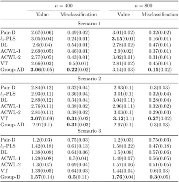
Table 2.1: Results of average means (standard deviations) of empirical value functions and misclas-sification rates for four continuous-outcome simulation scenarios with 40 covariates. The best value functions and misclassification rates are in bold.
n= 400 n= 800
Value Misclassification Value Misclassification Scenario 1
Pair-D 2.67(0.06) 0.49(0.02) 3.01(0.02) 0.32(0.02) l1-PLS 3.05(0.04) 0.24(0.01) 3.15(0.01) 0.16(0.01) DL 2.6(0.04) 0.54(0.01) 2.78(0.02) 0.47(0.01) ACWL-1 2.69(0.05) 0.46(0.01) 2.9(0.02) 0.37(0.01) ACWL-2 2.77(0.05) 0.43(0.01) 3.02(0.01) 0.31(0.01) VT 2.66(0.03) 0.5(0.01) 2.81(0.02) 0.45(0.01) Group-AD 3.06(0.05) 0.22(0.02) 3.14(0.03) 0.15(0.02)
Scenario 2
Pair-D 2.84(0.12) 0.32(0.04) 2.93(0.1) 0.3(0.03) l1-PLS 2.93(0.11) 0.36(0.04) 3.01(0.1) 0.32(0.04) DL 2.89(0.12) 0.34(0.04) 3.04(0.11) 0.28(0.04) ACWL-1 2.76(0.11) 0.38(0.02) 2.96(0.11) 0.32(0.02) ACWL-2 2.81(0.11) 0.38(0.02) 3.03(0.1) 0.29(0.03) VT 3.07(0.09) 0.31(0.02) 3.12(0.1) 0.27(0.02) Group-AD 2.97(0.1) 0.31(0.03) 2.97(0.1) 0.3(0.03)
Scenario 3
Pair-D 1.2(0.03) 0.75(0.03) 1.2(0.03) 0.75(0.03) l1-PLS 1.42(0.18) 0.61(0.13) 1.58(0.22) 0.47(0.18) DL 1.38(0.08) 0.64(0.06) 1.5(0.08) 0.57(0.06) ACWL-1 1.29(0.08) 0.7(0.04) 1.49(0.07) 0.56(0.05) ACWL-2 1.3(0.07) 0.69(0.04) 1.57(0.06) 0.51(0.05) VT 1.39(0.05) 0.64(0.03) 1.44(0.04) 0.6(0.03) Group-D 1.57(0.14) 0.5(0.11) 1.76(0.04) 0.3(0.05)
2.5.2 Study of Binary and Survival Outcomes
For the binary outcomeR, the dataset is independently generated by the logistic regression model
logit(P[Ri = 1]) =µ(xi) + K
∑
k=1
(xTi βk)I(A=k),
where the link function logit(x) = log1−xx. We consider same interaction effects as the first two scenarios of the continuous outcome simulation study.
Since pairwise D-learning and ACWL are not intended for the binary outcome, after modi-fying thel1-PLS by usingl1 penalized logistic regression (l1-PLR), we comparel1-PLR, DL and
VT with our AD-learning. Table 2.2 shows the value functions and misclassification rates for p= 40 andn= 400,800. We can see that our proposed AD-learning has largest value functions and lowest misclassification rates in both scenarios. Moreover, there are some mismatches in model based methods such asl1-PLS, where the misclassification rates and the value functions
tuning procedure in l1-PLS. The other potential reason is the mismatch between minimizing
prediction error and maximizing value function in model based methods.
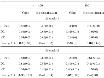
Table 2.2: Results of average means (standard deviations) of empirical value functions and misclassi-fication rates for two binary-outcome simulation scenarios with 40 covariates. The best value functions and misclassification rates are in bold.
n= 400 n= 800
Value Misclassification Value Misclassification Scenario 1
l1-PLR 0.88(0.01) 0.58(0.02) 0.91(0) 0.45(0.02) DL 0.85(0.01) 0.67(0.01) 0.87(0.01) 0.61(0) VT 0.84(0.01) 0.68(0.01) 0.84(0) 0.69(0) Binary-AD 0.9(0.01) 0.44(0.02) 0.92(0) 0.32(0.02)
Scenario 2
l1-PLR 0.83(0.01) 0.66(0.05) 0.86(0) 0.61(0.05) DL 0.81(0.01) 0.53(0.01) 0.85(0.01) 0.44(0.01) VT 0.83(0.01) 0.43(0.01) 0.83(0.01) 0.51(0) Binary-AD 0.86(0.01) 0.43(0.04) 0.87(0.01) 0.4(0.04)
Next we consider R to be the outcome of time to event. The simulated data are generated by the following model with the exponential distribution
Ri= exp(λi),
where exp denotes the exponential distribution andλi =µ(xi) +
∑K
k=1(xTi βk)I(A=k) for i=
1,· · · , n. The censoring time Ci;i= 1,· · ·, n, are generated from an exponential distribution
with mean θ to induce around 25% censoring rate. We consider the same settings as those in the binary case. For comparisons, we apply thel1 penalized CPH models and compare it with
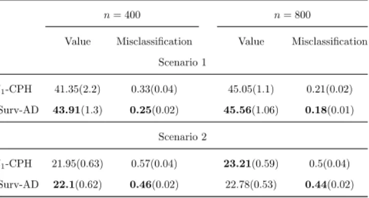
AD-learning, since other methods we use previously are not designed for the survival outcome. From Table 2.3 with p = 40, we can see that our proposed AD-learning has clear advantages overl1-CPH. In addition, we also observe the mismatch phenomena ofl1-CPH in Scenario 2 of
Table 2.3: Results of average means (standard deviations) of empirical value functions and misclassifi-cation rates for two survival-outcome simulation scenarios with 40 covariates. The best value functions and misclassification rates are in bold.
n= 400 n= 800
Value Misclassification Value Misclassification Scenario 1
l1-CPH 41.35(2.2) 0.33(0.04) 45.05(1.1) 0.21(0.02) Surv-AD 43.91(1.3) 0.25(0.02) 45.56(1.06) 0.18(0.01)
Scenario 2
l1-CPH 21.95(0.63) 0.57(0.04) 23.21(0.59) 0.5(0.04) Surv-AD 22.1(0.62) 0.46(0.02) 22.78(0.53) 0.44(0.02)
2.5.3 Study of High Dimensional Problems
We evaluate our AD-learning performance for high dimensional settings. We consider the sample size n = 400 so that each treatment group has roughly 100 patients and number of covariates p = 800. Scenarios 1-2, 3-4, 5-6 correspond to continuous, binary, and survival outcomes respectively. The interaction effects considered here are the same as the first two scenarios in the continuous setting in Section 5.1.
From Table 2.4, we can find that our proposed AD-learning performs better than l1-PLS.
Table 2.4: Results of average means (standard deviations) of empirical value functions and misclassifi-cation rates for six high dimensional simulation scenarios. The best value functions and misclassifimisclassifi-cation rates are in bold.
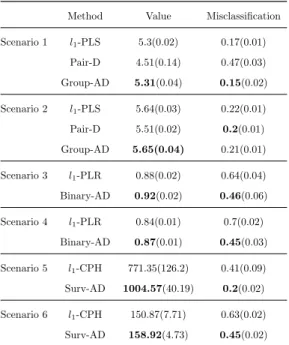
Method Value Misclassification
Scenario 1 l1-PLS 5.3(0.02) 0.17(0.01) Pair-D 4.51(0.14) 0.47(0.03) Group-AD 5.31(0.04) 0.15(0.02)
Scenario 2 l1-PLS 5.64(0.03) 0.22(0.01) Pair-D 5.51(0.02) 0.2(0.01) Group-AD 5.65(0.04) 0.21(0.01)
Scenario 3 l1-PLR 0.88(0.02) 0.64(0.04) Binary-AD 0.92(0.02) 0.46(0.06)
Scenario 4 l1-PLR 0.84(0.01) 0.7(0.02) Binary-AD 0.87(0.01) 0.45(0.03)
Scenario 5 l1-CPH 771.35(126.2) 0.41(0.09) Surv-AD 1004.57(40.19) 0.2(0.02)
Scenario 6 l1-CPH 150.87(7.71) 0.63(0.02) Surv-AD 158.92(4.73) 0.45(0.02)
2.6 Real Data Applications
In this section, we perform a real data analysis to further evaluate our proposed AD-learning. We consider a clinical trial dataset from “AIDS Clinical Trials Group (ACTG) 175” in (Hammer et al., 1996) to study whether there is a subgroup of patients suitable for different combination treatments of AIDS. In this study, with equal probabilities, a total number of 2139 patients with HIV infection were randomly assigned into four treatment groups: zidovudine (ZDV) monotherapy, ZDV combined with didanosine (ddI), ZDV combined with zalcitabine (ZAL), and ddI monotherapy.
We consider two outcomes for our analysis. The first outcome is the difference between the early stage (around 25 weeks) CD4+ T (cells/mm3) cell amount and the baseline CD4+ T cells prior to the trial. This was also studied in (Lu et al., 2013) and (Fan et al., 2017). Using this short term outcome, our goal is to use AD-learning to find the short term optimal IDR for each patient with AIDS among four treatment groups. We report the estimator of the coefficient wTi BT for each treatment in Table 2.5.
Table 2.5: Results of coefficients estimation for comparison functions.
Variable Name (1-7) ZDV ZDV+ddI ZDV+Zal ddI
Intercept −49.86 44.66 −3.53 8.73
Age −0.47 4.33 −3.34 −0.52
Weight 0 0 0 0
Karnofsky Score 0 0 0 0
CD4 baseline 3.58 −14.79 −14.78 9.46
Days pre-anti-retroviral therapy 0 0 0 0
Hemophilia 0 0 0 0
Homosexual activity −0.28 −3.96 0.65 3.60
History of drug use −2.50 8.20 4.03 −9.74
Race 0 0 0 0
Gender 0 0 0 0
Antiretroviral history 0 0 0 0
Symptomatic indicator 0 0 0 0