EARLY ASSESSMENT OF TUMOR RESPONSE TO RADIATION THERAPY USING HIGH-RESOLUTION CONTRAST ENHANCED ULTRASOUND IMAGING TECHNIQUES
AND APPLICATIONS FOR PROSTATE CANCER
Sandeep K. Kasoji
A dissertation submitted to the faculty of the University of North Carolina at Chapel Hill in partial fulfillment of the requirements for the degree of Doctor of Philosophy in the Department
of Biomedical Engineering in the School of Medicine.
Chapel Hill 2018
iii ABSTRACT
Sandeep K. Kasoji: Early Assessment of Tumor Response to Radiation Therapy Using Advanced Contrast Enhanced Ultrasound Imaging Techniques and Applications for
Prostate Cancer
(Under the direction of Paul A. Dayton)
Traditional anatomical imaging for cancer diagnosis and assessing response to therapy is limited to just the superficial appearance of a tumor. A functional imaging approach, which takes a closer at look various microenvironments within the tumor, is likely to offer a more holistic view of the tumor behavior and response to treatment. Acoustic Angiography is a novel super-harmonic contrast ultrasound imaging technique that utilizes a dual-frequency transducer to quickly generate high-resolution 3D microvascular images with exceptionally high contrast-to-tissue ratio. Herein, we demonstrate the ability of Acoustic Angiography to quantify tumor microvascular features and investigate their changes after therapeutic doses of radiation therapy in a tumor bearing rodent model. We then demonstrate using functional longitudinal data analysis that quantified microvascular features can be used to predict radiation therapy response with limited time point measurements.
iv
Acoustic Angiography hinges on certain design improvements, primarily increased depth of penetration. The last part of this dissertation discusses the development of a dual-frequency linear array transducer for Acoustic Angiography.
This dissertation consists of two primary hypotheses:
1) Acoustic Angiography can be used to quantify changes in tumor microvascular features and predict radiation treatment response earlier than using tumor volume alone.
v
This is dedicated to:
My wife, Dr. Meghana Konanur, who has been a constant source of love and encouragement throughout my academic career.
My family, who through their patience, guidance, love, and support, made this Ph.D. work possible.
vi
ACKNOWLEDGMENTS
I would like to first thank Dr. Paul Dayton, who has been an incredibly supportive adviser. His constant support and guidance throughout my graduate career is greatly appreciated and will always be remembered. I would next like to thank Dr. Sha Chang, whose enthusiasm for novel research has been the backbone for the first section of my thesis. I would like to thank the rest of my committee, Drs. Emily Chang, Xiaoning Jiang, and Ronald Chen, for their
indispensable guidance throughout this Ph.D. work in their respective fields of expertise.
I would next like to acknowledge all of my collaborators who made this work possible. Specifically, Drs. Sibo Li and Jinwook Kim for their expertise in novel transducer design, and Dr. Stuart Foster and his lab for their expertise in fabricating dual-frequency transducers. I would also like to thank all of the undergraduate students (Ruby Patel and Amit Cudykier) who I have had the pleasure of mentoring. They made significant contributions to data analysis that helped move these projects forward.
I would like to thank all of the past and current members of the Dayton Lab. I have learned a great deal from each and every one of them. Their kindness and friendship will always be remembered. Lastly, I would like to thank all of my friends and mentors who have acted as role models for me throughout my life. This work and many of my other accomplishments are a result of collective thought and collaboration.
vii
TABLE OF CONTENTS
ABSTRACT ... III
ACKNOWLEDGMENTS ... VI
TABLE OF CONTENTS ... VII
LIST OF FIGURES ... XIII
LIST OF TABLES ... XVI
LIST OF ABBREVIATIONS ... XVII
CHAPTER 1: OVERVIEW OF CANCER AND RADIATION THERAPY ... 1
1.1 CANCER AND THE ROLE OF ANGIOGENESIS ... 1
1.2 RADIATION THERAPY AND ITS EFFECT ON TUMOR MICROVASCULATURE ... 4
CHAPTER 2: OVERVIEW OF CANCER IMAGING ... 8
2.1 MODALITIES FOR CANCER IMAGING ... 8
2.2 IMAGING FOR ASSESSING RESPONSE TO THERAPY ... 9
2.3 MEDICAL ULTRASOUND IMAGING ... 11
2.4 ULTRASOUND CONTRAST IMAGING ... 13
CHAPTER 3: OVERVIEW OF HIGH-RESOLUTION CEUS ... 15
3.1 ACOUSTIC ANGIOGRAPHY ... 15
viii
3.3 PRIOR STUDIES WITH ACOUSTIC ANGIOGRAPHY ... 18
CHAPTER 4: AA FOR ASSESSING TUMOR MICROVASCULAR RESPONSE TO RT ... 20
4.1 OVERVIEW ... 20
4.2 MATERIALS AND METHODS ... 21
4.2.i Rat and Tumor Models ... 21
4.2.ii RT and Monitoring ... 21
4.2.iii Imaging Procedure... 24
4.2.iv Image Analysis ... 25
4.2.v Data Analysis ... 28
4.3 RESULTS ... 29
4.3.i TV and VVD Results ... 29
4.3.ii PN, SOAM, DM, and TCM Results ... 36
4.4 DISCUSSION AND CONCLUSIONS ... 37
CHAPTER 5: PRELIMINARY FUNCTIONAL PRINCIPAL COMPONENTS ANALYSIS ON LONGITUDINAL MICROVASCULAR IMAGING DATA SETS ... 43
5.1 OVERVIEW ... 43
5.2 FUNCTIONAL DATA ANALYSIS ON BIOLOGICALLY RELEVANT LONGITUDINAL DATA ... 44
5.3 METHODS ... 45
5.3.i Acquisition of Additional Data ... 45
5.3.ii Data and Statistical Analysis ... 45
5.4 RESULTS ... 48
ix
CHAPTER 6: EXTENSIONS, LIMITATIONS, AND FUTURE
DIRECTIONS ... 54
6.1 MOLECULAR IMAGING FOR ASSESSING RESPONSE TO RADIATION THERAPY ... 54
6.1.i Overview ... 54
6.1.ii Methods ... 56
6.1.iii Results and Discussion ... 58
6.2 CURRENT LIMITATIONS OF ACOUSTIC ANGIOGRAPHY AND IMPROVEMENTS ... 60
6.3 CEUS AND RADIOMICS ... 61
CHAPTER 7: IN-VITRO AND IN-VIVO TESTING OF A PROTOTYPE DUAL-FREQUENCY ARRAY TRANSDUCER ... 63
7.1 OVERVIEW ... 63
7.1.i Development of a Dual-Frequency Linear Array for Acoustic Angiography . 63 7.1.ii Dual-frequency Transrectal Ultrasound for Prostate Cancer Imaging ... 65
7.2 METHODS ... 67
7.2.i Verasonics Coding ... 67
7.2.ii DF-TRUS Development ... 68
7.2.iii Acoustic Characterization ... 70
7.2.iv In-Vitro Imaging ... 71
7.2.v In-Vivo Imaging ... 73
7.3 RESULTS ... 74
7.3.i Acoustic Characterization Results of DF-TRUS Transducer ... 74
7.3.ii In-vitro Experiment Results ... 76
7.3.iii In-Vivo Results ... 77
x
7.5 CONCLUSIONS ... 81
CHAPTER 8: PROOF OF CONCEPT DUAL-PROBE/ DUAL-FREQUENCY TRANSDUCER FOR AA... 82
8.1 OVERVIEW ... 82
8.2 METHODS ... 83
8.2.i Verasonics Coding ... 83
8.2.ii DP-DF Set-up ... 83
8.2.iii Acoustic Characterization ... 84
8.2.iv In-Vitro Imaging ... 85
8.2.v In-Vivo Imaging ... 86
8.2.vi Image Processing and Analysis ... 87
8.3. RESULTS ... 88
8.3.i Acoustic Characterization Results... 88
8.3.ii In-vitro Experiment Results ... 90
8.3.iii In-vivo Results ... 91
8.4 DISCUSSION AND CONCLUSIONS ... 94
8.5 FUTURE WORK ... 97
APPENDIX A: A QUANTITATIVE APPROACH TO CHARACTERIZING MALIGNANT RENAL CELL CARCINOMA USING CONTRAST ENHANCED ULTRASOUND ... 98
A.1 INTRODUCTION ... 98
A.2 MATERIALS AND METHODS ... 100
A.2.i Patient Recruitment and Initial Tests ... 100
xi
A.2.iii CEUS Time-Intensity-Curve Analysis ... 102
A.2.iv Histological Analysis ... 105
A.2.v Statistical Analysis ... 105
A.3 RESULTS ... 106
A.4 DISCUSSION ... 108
A.5 CONCLUSION ... 113
APPENDIX B: EFFICIENT DNA FRAGMENTATION IN A BENCH-TOP ULTRASONIC WATER BATH ENABLED THROUGH THE USE OF CAVITATION ENHANCING MICROBUBBLES AND NANODROPLETS ... 115
B.1 INTRODUCTION ... 115
B.2 METHODS ... 118
B.2.i Genomic DNA preparation ... 118
B.2.ii Microbubble and Nanodroplet Preparation ... 118
B.2.iii DNA Fragmentation: Covaris E110 Sonicator ... 119
B.2.iv DNA Fragmentation: Branson Sonifier Bath ... 120
B.2.v Next-generation Sequencing ... 120
B.3 RESULTS AND DISCUSSION ... 121
B.3.i Nanodroplets are a shelf-stable agent that perform better than microbubbles for DNA fragmentation ... 121
B.3.ii DNA fragmented in the presence of nanodroplets is consistent with DNA fragmented by a commercially available method ... 125
B.3.iii The addition of nanodroplets permits DNA fragmentation in a bench top ultrasonic water bath ... 129
B.4 CONCLUSION ... 133
xii
APPENDIX D: SUPPLEMENTARY TABLES ... 139
xiii
LIST OF FIGURES
Figure 3. 1. Acoustic Angiography and B-mode images. ... 15
Figure 3. 2. The RMV prototype dual-frequency probe used for AA imaging. ... 16
Figure 3. 3. The effect of frame averaging on AA images. ... 18
Figure 4. 1. Setup used for irradiation and ultrasound imaging... 23
Figure 4. 2. Summary of the image analysis for calculating VVD. ... 26
Figure 4. 3. An example of vessels segmented from an AA image. ... 27
Figure 4. 4. A comparison of TV and VVD by response group ... 30
Figure 4. 5. Example of VDD and TV growth curves ... 33
Figure 4. 6. A visual comparison of VVD and TV changes. ... 34
Figure 4. 7. Early detection of treatment failure by dose group. ... 35
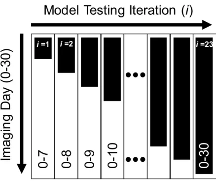
Figure 5. 1. Iterations of fPCA... 47
Figure 5. 2. Binomial Logistic Regression results. ... 48
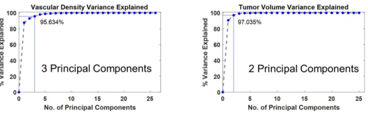
Figure 5.2. Scree plots for TV and VVD. ... 48
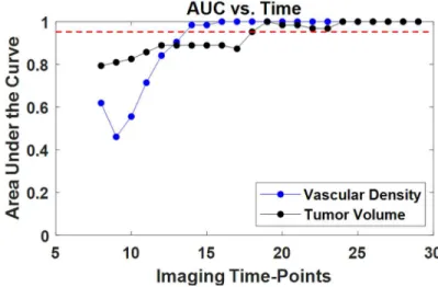
Figure 5. 3. Plots of AUC of ROC curves. ... 49
Figure 6. 1. USMI of a murine angiosarcoma model. ... 55
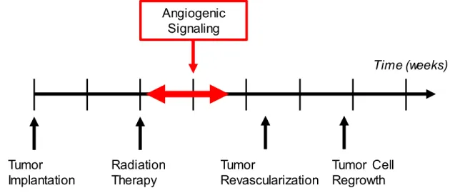
Figure 6. 2. Hypothesized molecular targeting signal timeline. ... 55
Figure 6. 3. Sample 2D images from 3D scans from a single tumor. ... 57
Figure 6. 4. Summary of average longitudinal curves of TV and USMI. ... 59
Figure 7. 1. Stacked element design. ... 69
Figure 7. 2. DF-TRUS prototype transducer. ... 70
Figure 7. 3. Setup for in-vivo imaging. ... 71
Figure 7. 4. Transmit and receive beam maps from the DF-TRUS transducer. ... 74
Figure 7. 5. The transmit waveform of the DF-TRUS. ... 75
xiv
Figure 7. 7. Lateral and axial resolution measurements of EV-8C4. ... 77
Figure 7. 9. 3D representation of the 3D image volume. ... 78
Figure 8. 1. 3D modeling of transmit and receive transducers for the DP-DF configuration. ... 84
Figure 8. 2. Transmit and receive beam maps from the DP-DF transducer. ... 88
Figure 8. 3. An alignment beam map of the DP-DF transducer in the elevational-axial plane. ... 89
Figure 8. 4. The transmit waveform of the DP-DF transducer. ... 90
Figure 8. 5. In-vivo images from the DP-DF, RMV, and EV-8C4 transducers. ... 92
Figure 8. 6. A Comparison of frame averaging versus no frame averaging using the DP-DF transducer. ... 93
Figure 8. 7. MIPs of the DP-DF probe compared with the RMV probe of the same FSA tumor. ... 93
Figure A. 1. Ellipsoidal ROI selection of both the lesion and normal renal cortex. ... 102
Figure A. 2. Sample TICs of a lesion and renal cortex. ... 105
Figure B. 1. Analysis of the fragmented DNA products following focused-wave sonication of purified genomic DNA. ... 122
Figure B. 2. Nanodroplets persisted in solution longer than microbubbles. ... 124
Figure B. 3. Nanodroplets are an effective cavitation agent for use in DNA fragmentation. ... 125
Figure B. 4. Saccharomyces cerevisiae genomic DNA (BY4741) fragmented with nanodroplets in a commercial sonicator is comparable in quality to DNA fragmented using a commercial method. ... 126
Figure B. 5. The addition of nanodroplets allows genomic DNA fragmenation in an ultrasonic water bath. ... 128
Figure B. 6. DNA fragmentation in an ultrasonic water batch compared to a commercially available device. ... 129
Figure B. 7. Saccharomyces cerevisiae genomic DNA (BY4741) fragmented with nanodroplets in an ultrasonic water bath is comparable in quality to DNA fragmented in a commercially available device. ... 131
Figure C. 1. Growth curves of PN and vessel tortuosity metrics. ... 134
xv
Figure C. 3. Transmit waveform of RMV probe. ... 136 Figure C. 4. The starch-iodine test was performed to confirm the presence
of cavitation. ... 137 Figure C. 5. CTR vs. Imaging Depth in an attenuating phantom of the
xvi
LIST OF TABLES
Table 4. 1 Treatment Response Statistics by Dose Group ... 29
Table 4. 2 Tumor Volume and Volumetric Vascular Density Growth Curve Statistics... 32
Table 4. 3. Average initial TV and VVD by dose group. ... 35
Table 7. 1 In-vivo Imaging Parameters. ... 86
Table A. 1. Definitions for metrics used for TIC analysis. ... 104
Table A. 2. Results from ten metrics derived from lesion and parenchyma TICs. ... 107
Table D. 1. Summary of SNR and CTR values for all probes for comparison. ... 139
xvii
LIST OF ABBREVIATIONS
2D Two-Dimensional
3D Three-Dimensional
AA Acoustic Angiography
AML Angiomyolipoma
A-T Adenine-Thymine
AUC Area Under the Curve
avβ3 Alpha-v-beta-3 integrin
B-mode Brightness Mode
ccRCC Clear Cell Renal Cell Carcinoma
CE Contrast Enhanced
CEUS Contrast Enhanced Ultrasound Imaging
ChIP Chromatin Immunoprecipitation
chRCC Chromophobe Renal Cell Carcinoma
CPS Cadence Pulse Sequence
CT Computed Tomography
CTR Contrast-to-Tissue Ratio
xviii
CTRImg Contrast-to-Tissue Ratio (measured with image data)
dB Decibel
DFB Decafluorobutane
DF-TRUS Dual-Frequency Transrectal Ultrasound
DICOM Digital Imaging and Communications in Medicine
DM Distance Metric
DMAS Delay-Multiply-and-Sum
DNA Deoxyribonucleic Acid
DP-DF Dual-Probe/Dual-Frequency
DRE Digital Rectal Examination
EV-8C4 (Siemens Prostate Transducer)
FDA Functional Data Analysis
FDG Fluorodeoxyglucose
FFT Fast Fourier Transform
fPCA Functional Principal Component Analysis
FSA Fibrosarcoma
FWHM Full-Width Half-Max
xix
gDNA Genomic DNA
Gy Gray (unit of ionizing radiation dose)
Hz Hertz (unit of frequency)
IQR Interquartile Range
IV Intravenous
MATLAB (Mathworks computational program)
MHz Megahertz (unit of frequency)
MI Mechanical Index
MIP Maximum Intensity Projection
MPa Megapascal
MRA Magnetic Resonance Angiography
MRI Magnetic Resonance Imaging
MV MegaVolts
MVm Microvascular metric
OCT Oncocytoma
OCT Optical Coherence Tomography
PACE Principal Analysis by Conditional Expectation
xx PCa Prostate Cancer
PCR Polymerase Chain-Reaction
PEG Polyethylene Glycol
PET Positron Emission Tomography
PI Peak Intensity
PN Percent Necrosis
pRCC Papillary Renal Cell Carcinoma
PSA Prostate Specific Antigen
PZT Lead Zirconate Titanate
RCC Renal Cell Carcinoma
RECIST Response Evaluation Criteria in Solid Tumors
RF Radio Frequency
RMV (Dual-element probe used for AA)
RNA Ribonucleic Acid
ROC Receiver Operator Characteristic
ROI Region of Interest
ROS Reactive Oxygen Species
xxi SBRT Stereotactic Body Radiotherapy
SNR Signal-to-Noise Ratio
SNRdB Signal-to-Noise Ratio (measured with voltage data)
SNRImg Signal-to-Noise Ratio (measured with image data)
SOAM Sum of Angles Metric
SPECT Single Photon Emission Computed Tomography
SRS Stereotactic Radiosurgery
SSD Source-to-Skin Distance
T80% Time to 80% on wash-out
T80%-r Time to 80% on wash-out ratio
TCM Total Curvature Metric
TE Tris-EDTA buffer
TIC Time Intensity Curve
TPk Time to Peak
TPk-r Time to Peak ratio
TRUS Transrectal Ultrasound
TUNEL Terminal deoxynucleotidyl
xxii
TVx Start of Tumor Volume Recurrence
V Volt
VVD Volumetric Vascular Density
VVDx Start of Volumetric Vascular Density Recurrence
WIS Wash-in Slope
WIS-r Wash-in Slope ratio
WIWOS-r Wash-in/Wash-out ratio
WOS Wash-out Slope
1 CHAPTER 1:
Overview of Cancer and Radiation Therapy
1.1 Cancer and the Role of Angiogenesis
It is expected that over 1.6 million new cases of cancer will be diagnosed in 2017 in the United States and over 12 million new cases worldwide, with an estimated number of deaths reaching over 600,000 and 7 million, respectively [1,2]. Cancer incidence and mortality increased significantly during the 20th century, most probably due to the surge in tobacco use and other health epidemics such as obesity, increased alcohol consumption, and poor western-type diets. While cancer rates have slowly declined since the 1990’s with improved diagnostics, treatment, and healthier lifestyles, it is still the second most deadly disease in America, after heart disease, claiming 1 out of every 4 deaths [3].
2
Cancer arises when mutations in the DNA of normal cells result in aberrant cellular growth and function. Mutations can be caused by both environmental factors and genetic disposition, however recent data has shown that most cancers arise from random DNA copying “mistakes” [6]. Native cellular repair mechanisms will usually fix these mutations at various checkpoints in the cell cycle, or the cell will undergo apoptosis to prevent further mitotic divisions of the abnormal cell. Defects or mistakes made in these repair mechanisms may result in accumulation of mutations drastically increasing the probability of cancer [7].
Mutated cellular DNA can lead to the deregulation of cell signal transduction pathways, such as RNA transcription, protein synthesis, resulting in the inactivation or overactivation of certain cellular processes [8]. Usually these sorts of modifications result in increased
proliferation of the aberrant cells and unsettles the balance of regulatory pathways that maintain homeostasis in the body. Hanahan et al proposed six “hallmarks of cancer” consisting of
molecular characteristics of the tumor microenvironment that contribute to the development and proliferation of tumors, one of which is aberrant angiogenesis.
Normal angiogenesis is precisely regulated by the expression of pro-angiogenic and anti-angiogenic factors. In normal tissue, the balance between the expression of both factors is shifted towards anti-angiogenesis resulting in mostly quiescent blood vessels [9]. Rapidly proliferating tumor cells will eventually become hypoxic as they grow beyond the diffusion limit of oxygen with the existing vascular supply, thus straining the metabolic processes of the neoplasm [10]. This oxygen and nutrient starvation caused by hypoxia is a major driving factor in the
upregulation of angiogenesis, resulting in a shift towards pro-angiogenic factors [9].
3
nature, resulting in excessive sprouting of disorganized, tortuous, and highly dense networks of vessels. While initially the newly stimulated angiogenesis increases oxygenation and nutrient delivery to a certain extent, the overall function of the tumor vasculature is deficient, suffering from leaky vessels and poor perfusion [11]. Further endothelial cell recruitment of pericytes ultimately results in the formation of premature vessels, as they are constantly bombarded with signaling factors preventing complete vessel maturation [12].
The rate and extent of angiogenesis varies by tumor type and the microenvironment conditions leading to tumors with a wide range of vascularity. The extent of tumor vascularity has significant implications on the growth of the tumor and the effectiveness of various treatment modalities, specifically chemotherapy and radiotherapy (RT). Chemotherapy (targeted or
untargeted), typically administered intravenously, requires sufficient blood flow into the tumor region for maximum effect. In addition to increased vascular density and tortuosity, angiogenesis is often accompanied with tumor hypoxia and necrosis [13]. Tumor necrosis has been reported to correlate with levels of angiogenesis and poor prognosis of malignant cancer. Specifically, αvβ3 integrin, a key regulator in tumor angiogenesis is known to be associated with necrosis and apoptotic activity [14]. Therefore it is typical for tumors to develop necrotic and perinecrotic regions of the tumor. Since a higher density of vessels exist in the perimeter of the tumor,
4
Usually, these techniques are used together with other treatment strategies such as radiation or surgical resection.
Similarly, presence of blood as an oxygen carrier increases the efficacy of RT by increasing oxygen radical formation, an indirect mechanism for radiation assisted cell death. Microvessel density and perfusion have been shown to be a prognostic factor of RT response. Previous studies have demonstrated the radioresistance of hypovascular/hypoxic tumors as well as the improvement in RT response with pro-angiogenic pre-treatment of the tumor prior to radiation. Other studies have proposed the delivery of secondary oxygen carriers via IV or intratumoral injection to increase oxygen concentration for increasing radiosensitivity [17].
1.2 Radiation Therapy and its Effect on Tumor Microvasculature
RT is one of the most basic forms of cancer treatment, used to treat approximately 50% of all cancer patients during their first course of treatment, and contributes to 40% of curative cancer treatment [18,19]. Approximately 40% of cancer patients are on at least their second course of RT, with rates of cancer resistance ranging from 20-30% for PCa, 10% for breast cancer, and as high as 90% for some types of lung cancer [20–23].
5
or single and double-strand breaks. Although direct ionization occurs, it only accounts for a small contribution of the total DNA damage [24]. Ionization can also pass through the cellular membrane, interacting with aqueous molecules and forming reactive oxygen species (ROS) and free radicals. ROS and free radicals are extremely reactive (given their unpaired electrons) and readily attack covalent bonds of DNA, causing single and double-strand breaks [25]. This accounts for the majority of DNA damage (>80%) and is the most commonly accepted
mechanism for cellular death. Cellular repair mechanisms (base excision repair) deal with base-pair deletions and single-strand breaks on a daily basis due to natural production of ROS and free radicals; however, repair of double-strand breaks is prone to errors and usually results in cellular apoptosis. Although some normal cell damage is inevitable during RT of cancer, it has been reported that highly proliferating cells such as cancer are more sensitive to radiation. Cellular death from radiation exposure occurs during the mitotic phases, therefore quickly dividing cells react sooner than healthy tissue [26]. The same phenomenon holds true for other quickly
dividing cells such as epithelial and endothelial cells.
To date, the clinical standard for assessing radiation treatment response is a system similar to Response Evaluation Criteria in Solid Tumors (RECIST), where changes in tumor size indicate positive or negative treatment response [27]. Unfortunately, gross changes in tumor volume (TV) occur very slowly (weeks to months after treatment) and is a limitation especially when the tumor is not responding well to the treatment as early assessment of a failed treatment will allow physicians more time to switch treatment strategies. Advances in radiobiology over the last half-century had revealed that changes in TV are the result of a long cascade of intricate biological processes. Better understanding the effect of radiation on various tumor
6
assessment of response to therapy, improving the effectiveness of adjuvant therapies, or developing more advanced methods of RT. One such microenvironment, the tumor
microvasculature, has been known to be significantly affected by radiation, resulting in a series of molecular changes that result in tumor cell death and control [28]. Endothelial apoptosis of tumor microvasculature is known to be a homeostatic factor in the regulation of tumor growth and is strongly correlated with tumor control when treated with radiation, therefore suggesting that DNA damage and consequential cell death due to exposure to ionizing radiation may not be the only significant factor determining the effect of RT [29]. Better understanding the complex mechanisms behind the microvascular response to radiation may enable a better understanding of overall tumor response to treatment, allowing for improved treatment planning.
Immediate changes in tissue perfusion as a result of cancer treatments have been closely studied and documented previously. In the context of RT, many studies have observed changes in vascular function in both clinical and pre-clinical studies. Park et al reported in an extensive review that lower dose treatments (<10 Gy) induced mild vascular damage, while larger doses (>15 Gy) resulted in significant vascular damage that was reflected in both vessel density and perfusion [30]. Long term vascular changes in higher-dose scenarios have been largely
consistent. In another study, it was reported that 10 Gy radiation induced an increase in perfusion immediately after radiation, and then a significant decrease in perfusion 26 hours post treatment. Perfusion returned to normal levels 7-11 days after treatment [31]. Others have reported similar trends in blood perfusion: a sudden hyper-perfusion, followed by a sudden hypo-perfusion, and then gradual return to normal perfusion levels.
7
predictor of long-term treatment response. It was reported by that immediate vascular volume and perfusion changes following high dose (>10 Gy) RT precede long term outcomes.
Specifically, a marked increase in perfusion and neovascularization was a potential predictor of long-term tumor regrowth [32–34]. This was corroborated by Song et al, who also reported increased revascularization in tumors that regrew 15 days after 30 Gy treatment [30]. Interestingly, Maeda et al demonstrated early microvascular changes (within just 2 days) in response to a single dose of radiation in a mouse optical window chamber model suggesting that the tumor microvasculature is a highly dynamic and responsive system [35].
In addition to functional changes in tissue microvasculature, previous studies have
reported changes in vessel structure in response to RT. Specifically, Bullitt et al demonstrated the use of vessel segmentation and tortuosity calculations from magnetic resonance angiography (MRA) images of the brain and correlated radiation treatment outcome with vascular
8 CHAPTER 2:
Overview of Cancer Imaging
2.1 Modalities for Cancer Imaging
Cancer can be diagnosed using a variety of techniques including blood tests, physical examination, tissue biopsy, genetic tests, and imaging. Technology is rapidly improving in all of the diagnostic areas whether it is the development of antibodies that are more specific to blood serum antigens or advancements in Next Generation Sequencing/High-throughput Sequencing for personalized cancer screening [37–39]. Radiology plays an important role in the
multidisciplinary approach to cancer diagnosis and disease management; it has dominated the area of cancer diagnostics for over half a century due to its non-invasiveness, standardized techniques, and versatility in application. Imaging is applied in a number of ways in oncology, including routine screening, biopsy guidance, and treatment monitoring to name a few. Nearly every imaging modality is currently used in cancer diagnosis (ultrasound, computed tomography (CT), magnetic resonance imaging (MRI), positron emission tomography (PET), single photon emission computed tomography (SPECT), bone scans, Optical Coherence Tomography (OCT), each with its unique strengths and weaknesses [40–42].
9
depending on the type and location of the tumor. Traditional grayscale ultrasound imaging is useful for imaging soft tissue tumors with high sensitivity which may otherwise be difficult to see with x-ray imaging. It is a real-time imaging modality, inexpensive, and globally accessible. CT and MRI excel at allowing physicians to perform 3D full body imaging of the body to visualize location, morphology, and size of lesions [43].
Functional imaging adds an additional dimension to cancer diagnosis by offering information regarding the molecular activity of the cancer. Two examples include PET and SPECT imaging, which can be used to identify regions of abnormal molecular activity (e.g. localized increase in radiolabeled glucose uptake is indicative of cancer). While PET and SPECT have high sensitivity and specificity to the radiolabeled compounds that are used for imaging, they lack resolution and anatomic detail. Development of multimodal imaging techniques, such as PET-CT or PET-MRI have made it possible to visualize anatomical and functional
information simultaneously [43]. The fusion of anatomical and functional imaging has been the backbone of image aided cancer diagnostics, and the same theories can be applied to assessing cancer response to therapy as well.
2.2 Imaging for Assessing Response to Therapy
The long standing standard for assessing treatment response is quantifying changes in the size of the tumor mass. Since tumor measurements can be easily performed serially and
10
demonstrated that volumetric measurements may provide a more accurate assessment. The Response Evaluation Criteria in Solid Tumors (RECIST) was published in 2000 as a guide of international standards for assessing tumor response to therapy using medical imaging, specifically CT and MRI. It is commonly used by physicians on a daily basis as part of their treatment monitoring (which also includes symptom surveillance and other tests). RECIST categorizes lesions as measurable and non-measurable. Measurable lesions are >20 mm on chest x-ray (or >10 mm on spiral CT) [27]. Measurable lesions are further categorized as complete response, partial response, stable disease, or progressive disease based on percent increase or decrease of the sum of the largest diameters. Non-measurable, or non-target lesions are also categorized as complete responders, stable disease, or progressive disease based on their disappearance or persistence, or the appearance of new lesions.
The advancement of new cancer drugs and targeted treatment strategies has warranted the development of a new method of assessing tumor response. At the time RECIST was published, many of the chemotherapeutics used were cytotoxic drugs which functioned by directly killing cancer cells. Therefore, a change in the number of cancer cells was represented by a change in the TV. New treatment strategies, such as anti-angiogenic drugs, or drugs that inhibit cancer cell proliferation by interrupting relevant cell signaling pathways, do not directly kill the cancer cells yet have still demonstrated sufficient tumor control and disease management [44]. Considering the effects of these new types of treatments requires a different biomarker that looks beyond the size of the tumor.
11
for PET imaging to assess glycolytic metabolism of the tumor [45]. PET is often coupled with an anatomical imaging modality such as PET-CT or PET-MRI which registers the molecular
(functional) information with the anatomy.
Dynamic contrast-enhanced CT and MRI enable quantification of contrast perfusion in the tissue of interest [46]. Depending on the type of therapy, blood perfusion in the tumor may be expected to increase or decrease. For example, a decrease in tumor perfusion might be expected after the delivery of an anti-angiogenic drug. Changes in tumor metabolism and blood perfusion are two of many alternative biomarkers that can be used for assessing response to therapy that may paint a more accurate picture of treatment effects than TV.
As discussed previously, angiogenesis plays a crucial role in tumor development and the resulting tumor vasculature has distinctive characteristics such as increased tortuosity, density, and permeability. Angiogenesis can be quickly triggered in response to physiological stimuli such as inflammation and hypoxia [47]. Since these changes have been shown to occur much sooner than the physical growth of the tumor mass itself, the ability to assess microvascular changes related to a particular disease would potentially increase the sensitivity of diagnostics and improve disease management.
2.3 Medical Ultrasound Imaging
12
of less than 1 m3, and requires just a small consult room. Recent advancements in ultrasound instrumentation have condensed the size of an ultrasound scanner to the size of a table or phone--in fact, there are now ultrasound apps that are available for the iPhone. This is phone--in contrast to CT, MRI, and nuclear imaging, which require significantly more expensive equipment and dedicated facilities to house the scanners. These large imaging rooms are usually equipped with a
procedure room and an external control room so that interference from ionizing radiation or magnetic fields do not affect bystanders or other unprotected equipment. Ultrasound is also significantly inexpensive. Standard diagnostic ultrasound and chest x-ray cost $150-300, while MRI, CT, and nuclear imaging can cost anywhere from $500-$2,500 depending on the
application (prices based on no insurance coverage) [48].
Medical ultrasound is most commonly used for anatomical imaging. Unlike the full-body imaging capabilities of CT and MRI, ultrasound has an extremely limited field of view of ~2-7 cm laterally, and 15-20 cm axially. However, ultrasound offers higher resolution, anywhere from 100-1000 µm depending on the desired frequency and application. In terms of cancer imaging, traditional brightness mode ultrasound (b-mode or gray-scale ultrasound) can detect abnormal lesions with high sensitivity, however it has low specificity in lesion subtyping or assessing malignancy [49]. It is also difficult to visualize blood with conventional ultrasound, and standard Doppler techniques are limited and unable to detect smaller vessels due to limited scattering of blood components and a low impedance mismatch between blood and the surrounding tissue.
13
for contrast enhanced ultrasound imaging (CEUS) which provides sufficient contrast between blood and the surrounding tissue.
2.4 Ultrasound Contrast Imaging
Microbubble contrast agents are composed of an inert, high molecular weight gas core stabilized by a phospholipid or albumin shell. Other molecules may be incorporated with bubble shell. For example, polyethylene glycol (PEG) is often incorporated into lipid shell
microbubbles, which acts as a stealth agent, reducing its visibility to the reticuloendothelial system. The bubbles are on the order of 1-3 µm in diameter, roughly the size of red blood cells [50]. This means that once introduced into the vascular supply, they remain strictly an
intravascular contrast agent. This is in contrast to gadolinium and iodine based contrast agents for CT and MRI, which eventually diffuse out of the vasculature. As a pure intravascular agent, the microbubbles increase the specificity of microvessel detection using ultrasound. The half-life of the bubbles is on the order of 3-5 minutes, depending on the organism that is being imaged; for humans, it is approximately 3 minutes. The shell components are cleared by the body through the liver and spleen, while the core gas is transferred out through the lungs and simply breathed out.
14
reflections centered at the fundamental frequency with weak higher harmonic signal. Various ultrasound algorithms take advantage of the non-linear oscillations for contrast imaging. For example, pulse inversion is a technique where two consecutive pulses (the second pulse is inverted) are transmitted such that their echoes are summed, subtracting the odd harmonics and summing the resultant even harmonics [52]. This effectively removes the linear fundamental frequency, while retaining the non-linear, harmonic (primarily 2nd order) signals.
CEUS has been used heavily in echocardiography, and in the last decade, techniques such as perfusion imaging and molecular imaging have been tested in preclinical and clinical settings in a variety of organ systems and cancer types [50]. While the applications of CEUS are
15 CHAPTER 3:
Overview of High-Resolution CEUS
3.1 Acoustic Angiography
Acoustic Angiography (AA) is CEUS imaging technique developed by the Dayton Lab at the University of North Carolina at Chapel Hill that implements the concept of superharmonic imaging, which utilize the broadband microbubble response for high-resolution microvascular imaging [56].
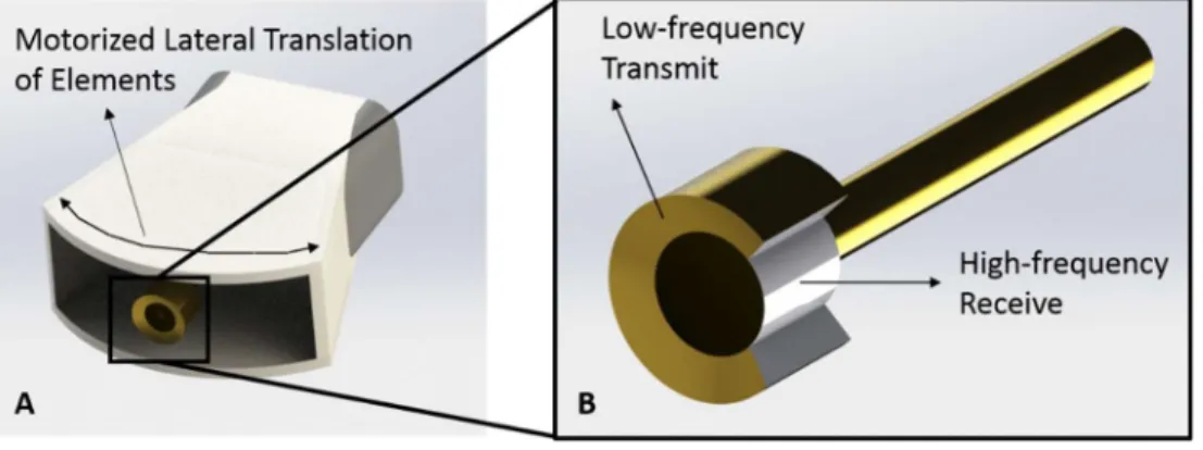
Figure 3. 1. Acoustic Angiography and B-mode images. A) B-mode image in the coronal view of a tumor located in the right flank of a rat indicated with yellow arrows. B) A coronal maximum intensity projection of 3D intensity data from a stack of 2D AA images in the same imaging area. Using AA we can visualize the tumor tissue and microvasculature with exceptional tissue
rejection.
16
microbubble response spans as high as the 8-10th order harmonics. The lower harmonics (mostly containing tissue signal) are filtered out using a high-pass filter. Since such broadband
transducers do not exist that can perform both a low frequency transmit and a high frequency receive, a prototype confocal dual-frequency transducer was developed containing a low
frequency (1-4 MHz, close to microbubble resonance) outer ring element for transmission and a high-frequency (25-30 MHz) inner element for receiving (Figure 3.2). The large bandwidth separation of the transmit and receive frequencies enables the detection of broadband
microbubble signals while rejecting linear tissue signal. AA is significantly more sensitive to microbubble contrast agents resulting in a high contrast to tissue ratio (CTR) of up to 20 dB, and because such a high receiving frequency is used, the resolution is approximately 100-200 µm, higher than conventional contrast imaging techniques [54].
17
3.2 Vascular Metrics Derived from Acoustic Angiography
A stack of 2D images acquired by translating the ultrasound probe in the elevational dimension can be constructed into a 3D visualization of tissue microvasculature. There are several vascular metrics that can be derived from AA 3D data. Using the grayscale 8-bit raw intensity data, thresholding algorithms can be used to filter out weak microbubble contrast signal from slow-flowing unresolvable vessels, below the resolution limit of AA and binarize the remaining resolvable vessels (>100 µm) -- this is performed over the entire 3D volume. For instance, volumetric vascular density (VVD) can be measured with the binarized image by summing the number of pixels above the grayscale threshold and dividing by the number of pixels within the user defined region of interest (ROI) encompassing the tumor region [57].
Individual resolvable vessels can also be segmented using specialized segmentation software, which generates an array of 3D vectors representing the tubular centerline for each vessel enabling quantitative morphological assessment. As discussed previously in section 2.1, tumor vessels are often characterized as highly tortuous. Using AA and segmentation methods, we calculate vessel tortuosity using three metrics: distance metric (DM), sum of angles metric (SOAM), and total curvature metric (TCM) [58]. The DM is calculated by dividing the length of the extracted vessel path by the length of the end-to-end vessel secant. The SOAM is calculated by integrating the angular changes throughout the centerline of the vessel, divided by the length of the extracted vessel path. TCM is calculated by summing the total curvature of the vessel and dividing by total path length [58]. All three metrics are complementary to describing vessel tortuosity—for example, SOAM and TCM are more sensitive to tightly coiled vessels.
18
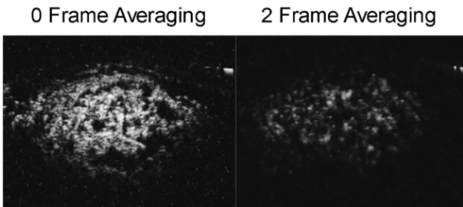
prognosis. By reducing the frame-rate of imaging, we can increase our sensitivity to microbubble signal, including signals from smaller, slow flowing vessels (Figure 3.3). This results in an image similar to conventional CEUS, however the increased resolution and contrast sensitivity allows us to draw precisely defined lines of regions of necrosis and calculate percent necrosis (PN). Using a slower frame-rate image, we apply the same binarization algorithm used for VVD calculations and count the pixels below the grayscale threshold.
Figure 3. 3. The effect of frame averaging on AA images. The AA image on the left was
acquired without frame averaging. Contrast signal from microvessels below the resolution limit can be detected. In this way, areas of no perfusion (considered severely hypoxic or necrotic) are easily discernable and can be extracted and measured using basic image processing. The image on the right is after 2 frame averaging. The signal intensity is significantly lowered since signal from small, slower flowing vessels is averaged out between frames. The result is that individual vessels can be visualized during 3D reconstruction.
3.3 Prior Studies with Acoustic Angiography
19
detect statistical increases in DM and SOAM in tumors as small as 2-3 mm [60]. This established the detection of “pre-palpable” tumors using quantification of microvascular features alone.
The work discussed in this dissertation builds upon this previous work and extends the application of AA to assessing tumor microvascular response to treatment, specifically RT. We investigate the quantification of various vessel features and evaluate their sensitivity to
20 CHAPTER 4:
AA for Assessing Tumor Microvascular Response to RT1
4.1 Overview
Previously we have demonstrated the ability to discriminate healthy from cancerous tissue solely by quantifying abnormal microvasculature using AA. As tumors develop, their microenvironment become denser with tortuous and leaky vessels. Additionally, quickly growing tumors become hypoxic resulting in regions of severe hypovascularity and necrosis. We
hypothesize that changes detected in the tumor microvascular microenvironment using AA in response to RT are correlated with long term survival. In this study, we longitudinally performed AA imaging on tumor bearing rats treated with a single dose of RT, measured five tumor
vascular features at each time point, and determined the correlation with long term survival compared with TV measurements.
21 4.2 Materials and Methods
4.2.i Rat and Tumor Models
All animal surgical and imaging procedures were reviewed and approved by the
University of North Carolina at Chapel Hill Animal Care and Use Committee prior to conducting this study. Rat FSA tumor tissue was subcutaneously implanted in the right flank of 30 female Fisher 344 rats as previously described [61]. Rat FSA was originally induced and isolated from Fisher 344 rats injected with the carcinogen, methylcholantrene [62]. Rat FSA is characterized as a local, non-metastasizing tumor that is highly vascular and oxygen dependent [62,63]. Because of its high vascularity, it is an appropriate tumor model for AA imaging after RT, since we are specifically interested in the tumor vascular response to therapy. Because rat FSA is oxygen dependent, avascular regions typically undergo tissue necrosis [63].
4.2.ii RT and Monitoring
22
dependent correlation between TV change and microvascular change for both complete response and partial response groups with similar statistics.
The rats were anesthetized using vaporized isoflurane and oriented in the left lateral recumbent position on a heating pad throughout the duration of the treatment with front and rear paws stabilized on the heating pad with medical tape. Positioning was performed using a
23
24
4.2.iii Imaging Procedure
Rats were imaged immediately prior to radiation for baseline measurements. After the radiation treatment, imaging was performed daily for 3 consecutive days and then every 3 days for approximately 30 days or until the tumors reached the maximum size of 2 cm in the longest diameter.
25
averaging with a frame rate of 3 frames/second was used for all AA imaging to improve the signal-to-noise ratio for producing optimal images.
4.2.iv Image Analysis
The b-mode images were used to calculate TV. The caliper feature on the Vevo 770 imaging software was used to measure the longest tumor diameter in each image axis to approximate the ellipsoidal volume of the tumor. The AA images were post-processed using MATLAB (MathWorks, Natick, MA), TubeX, and VesselView to measure VVD, PN, and vessel tortuosity through the SOAM, DM, and the TCM [65,66].
It is important to identify and remove large hypoechoic regions to not overestimate the total perfused tissue volume [67,68]. We assumed that large hypoechoic regions were due to necrosis and hypoxia, based on tumor ex vivo observations and prior literature that describes rat FSA as a highly oxygen dependent tumor [63]. These hypoechoic regions will be referred to as “necrotic” for simplicity, which encompasses necrotic and perinecrotic regions. For identifying necrotic regions, a de-noising 2D median filter was applied to each frame of the AA image slices to smooth the image and then a threshold was used to create a volumetric binary mask which identified large dark regions. The ratio of the number voxels representing necrotic regions within the ROI and the number of voxels representing the entire tumor ROI was calculated as PN.
𝑃𝑒𝑟𝑐𝑒𝑛𝑡 𝑁𝑒𝑐𝑟𝑜𝑠𝑖𝑠 (𝑃𝑁) = # 𝑣𝑜𝑥𝑒𝑙𝑠 𝑜𝑓 𝑖𝑑𝑒𝑛𝑡𝑖𝑓𝑖𝑒𝑑 𝑛𝑒𝑐𝑟𝑜𝑠𝑖𝑠 # 𝑜𝑓 𝑣𝑜𝑥𝑒𝑙𝑠 𝑖𝑛 𝑡ℎ𝑒 𝑡𝑢𝑚𝑜𝑟 𝑅𝑂𝐼
26
Otsu threshold method [69]. VVD was calculated by dividing the number of voxels representing vessels by the number of voxels representing the tumor tissue sans necrosis (Figure 4.2).
Figure 4. 2. Summary of the image analysis for calculating VVD. A single 2D slice of a 3D volume is shown in this figure. A) The original AA ROI. B) The original image, de-noised with a 2D median filter. C) The binary vessel image of the original ROI produced by applying an Otsu threshold. D) The hypoechoic mask made by applying a threshold on the de-noised image (B). E) The mask (D) applied to the binary vessel image (C). Arrows indicate resolvable vessels that have been converted into binary by thresholding.
27
vessels far from the tumor region reduces the sensitivity of detecting changes in tortuosity. The raw image ROI data was preconditioned into isotropic voxels prior to segmentation. The
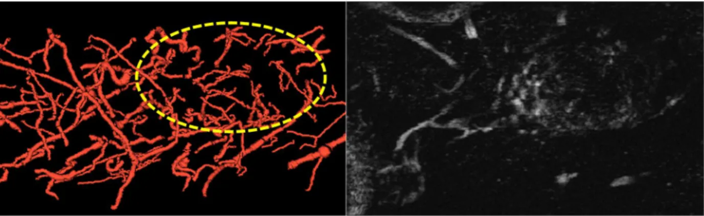
automatic, single vessel segmentation algorithm requires a manual definition of a seed point (performed by clicking a potential vessel in either the coronal or axial slice mode), which then automatically extracts the rest of the vessel by following the image intensity ridge representing the centerline of the calculated tubular structure (Figure 4.3). The algorithm performs a spatial up-sampling function which smooths the trajectory of each vessel. The radii of the vessel is also determined at each centerline point [66]. Initially for each image, approximately 100-200 vessels were segmented but were later filtered based on segment length to remove vessels that were too short to perform tortuosity metrics. A threshold vessel length of 500 points was used for all tortuosity analyses. The segmented data was imported into a second analysis software
(VesselView) also developed by Bullitt and Aylward, which calculated SOAM, DM, and TCM (among other metrics) for each vessel.
28
4.2.v Data Analysis
At the end of the study, treated rats were retrospectively categorized based on the treatment outcome as either partial response (initial treatment response followed by tumor recurrence) or complete response (full treatment response resulting in complete tumor disappearance). The 20 Gy study was terminated early at day 20 due to imaging schedule constraints. All complete responders were monitored for the duration of the study (30 days) for tumor regrowth, followed by an additional 30 days.
TV and all microvascular metric (MVm) (VVD, PN, SOAM, DM, TCM) growth curves for all individual rats were normalized by their respective baseline (pre-treatment) values. Initial TV growth curves (before tumor regression) and tumor recurrence rates were characterized by calculating their doubling times (Dt) using the equation:
Dt = (T – T0) × (log(2)/log(Vf)) – log(V0) (Dt – doubling time; T0 – time of initial
measurement; T – time of initial measurement; V0 – initial volume; Vf – final volume)
Similarly, TV regression was characterized by calculating the tumor halving times (Ht)
using the equation:
Ht = (T – T0) × (log(1/2)/log(Vf)) – log(V0) [70] (Ht – halving time; T0 – time of initial
measurement; T – time of initial measurement; V0 – initial volume; Vf – final volume)
Different phases of the MVm (initial response, regression, and recurrence phases) were characterized using linear regression.
29
metrics as well (labeled collectively as MVmx). Statistical differences in growth curves and TVx and MVmx values were evaluated using the Mann-Whitney U-test, and differences observed between dose groups were evaluated with the Kruskal-Wallis test, followed by the Tukey Post-Hoc multiple comparison test (α = 0.05). All statistical analysis was performed in MATLAB.
4.3 Results
4.3.i TV and VVD Results
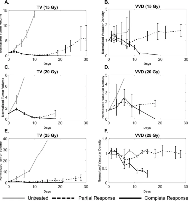
The treatment response statistics and sample sizes for each dose group are summarized in Table 1. Partial responders, complete responders, and untreated tumors in each dose group present distinctly different VVD and TV growth curves (Figure 4.4).
Table 4. 1 Treatment Response Statistics by Dose Group
15 Gy 20 Gy 25 Gy
Partial Response 5 (63%) 3 (60%) 3 (38%)
Complete Response 3 (38%) 2 (40%) 5 (63%)
Total Treated Tumors: 8 5 8
30
Figure 4. 4. A comparison of tumor volume (A, C, E) and tumor microvascular density (B, D, F) growth curves for complete responders (solid black), partial responders (dotted black), and untreated tumors (solid gray) for each dose group. Sample sizes for complete and partial
responders, and untreated groups were 3, 4, and 2 for the 15 Gy group, 2, 3, and 5 for the 20 Gy group, and 5, 3, and 2 for the 25 Gy cohorts, respectively. Error bars represent standard
deviation. Partial responders undergo a transient decrease in vascular density that correlates with tumor regression and eventually increases, correlating with tumor recurrence. For complete responders, both TV and VVD decrease. The large error bars in TV and VVD curves are expected due variability in tumor growth as well as heterogeneity of vascular supply.
0 10 20 30
Days 0 5 10 15 N o rm al iz e d T u m o r V o lu m e
TV (15 Gy)
0 10 20 30
Days 0 1 2 3 N o rm al iz e d V a sc u la r D en s it y
VVD (15 Gy)
0 10 20 30
Days 0 2 4 6 8 N o rm al iz e d T u m o r V o lu m e
TV (20 Gy)
0 10 20 30
Days 0 10 20 30 40 N o rm al iz e d T u m o r V o lu m e
TV (25 Gy) A. C. E. B. D. F.
31 Initial Response
Untreated tumors underwent normal, uninterrupted exponential volume growth with a mean doubling time of 1.9 ± 0.5 days (median: 1.9 days; range: 1.4 days; IQR: 0.6 days). All treated tumors presented delayed TV growth after the treatment (day 0) until day 3, at a growth rate significantly less (p=0.009) than compared to the untreated tumors with a mean tumor doubling time of 3.8 ± 2.6 days (median: 3.2 days; range: 11.7 days; IQR: 2.0 days). There was a non-significant decrease in the average tumor doubling time for treated tumors as RT dose increased. VVD of all treated tumors increased by an average of 18 ± 13%, significantly greater (p=0.023) than in untreated tumors, which increased by 4 ± 6%. There were no significant VVD or TV differences between partial and complete responders within each dose group (Table 2).
Tumor Regression
By day 5, all treated tumors experienced tumor regression where both TV and VVD decreased. There was no statistical difference in the regression rates of either TV or VVD between complete and partial responders in the 15, 20, and 25 Gy treatment groups. For
32
Table 4. 2 Tumor Volume and Volumetric Vascular Density Growth Curve Statistics
Untreated All
Treated 15 Gy 20 Gy 25 Gy
Complete Response Partial Response Complete Response Partial Response Complete Response Partial Response
Tumor Volume Doubling time – Initial Response
(days)
1.9 ± 0.5 3.8 ± 2.6
(p=0.009)
5.6 ± 3.4 3.4 ± 0.5 2.4 ± 1.4
5.5 ± 1.2 5.7 ± 4.7 3.6 ± 0.7 3.3 ± 0.3 2.3 ± 1.3 2.4 ± 1.9
Volumetric Vascular Density increase – Initial Response
(%)
4.3 ± 6.1 18.1 ± 12.7
(p=0.023)
21.0 ± 15.8 26.5 ± 10.2 10.0 ± 5.1
22.3 ± 21.3 20.5 ± 14.0 23.8 ± 15.3 28.3 ± 8.9
8.6 ± 5.9 12.4 ± 2.9
Tumor Volume Halving time – Regression
(days)
~ 3.0 ± 1.0 3.2 ± 0.7 2.8 ± 0.3 2.9 ± 1.4
2.5 ± 0.3 3.8 ± 0.5 3.0 ± 0.6 2.7 ± 0.1 2.1 ± 0.3 1.3 ± 1.6
Volumetric Vascular Density Regression (%)
~ -12.8 ±
9.3
-10.9 ± 4.9 -20.9 ± 14.7 -9.3 ± 5.0
-10.4 ± 6.1 -11.7 ± 3.5 -26.0 ± 19.6 -17.5 ± 14.1 -11.1 ± 5.7
-6.2 ± 1.0
Tumor Volume Doubling time – Recurrence
(days)
~ 4.7 ± 2.1 3.6 ± 0.8 6.4 ± 3.4 4.5 ± 1.2
Volumetric Vascular Density Recurrence (%)
~ 5.2 ± 3.2 7.2 ± 3.6 4.7 ± 3.3 3.2 ± 1.4
33 Tumor Recurrence
All partial responders rebounded and recurred between days 10 and 20 as indicated by their TV growth curves. VVD began to increase between days 7 and 11 and was also associated with tumor recurrence. Tumor recurrence occurred (non-significantly) earlier as dose increased as indicated by decreasing average TVx; VVD recurrence (average VVDx) was not statistically different between dose groups. When comparing TV and VVD curves for each individual tumor, the increase in VVD was observed earlier than the increase in TV (Figure 4.5). Figure 4.6
visually illustrates TV and VVD changes where VVD begins to increase while TV is still in the regression phase (Figure 4.6).
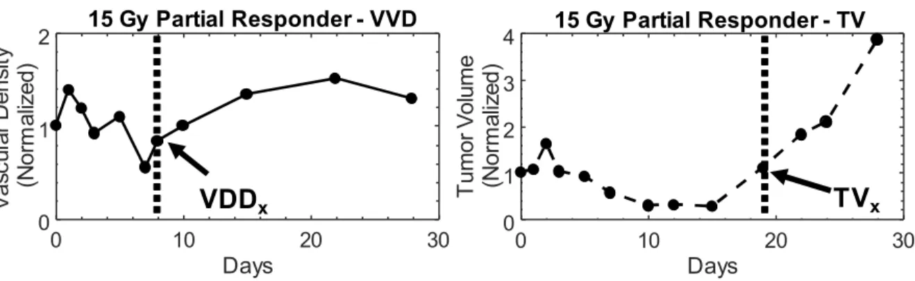
Figure 4. 5. Example of vascular density (left) and tumor volume (right) growth curves from a 15 Gy partial responder. All measurements were normalized to baseline values. In this particular partial responder failure, vascular density begins to increase as early as day 8, while tumor volume regrowth occurs later. The increase in the growth curve for both metrics demarcates the recurrence phase for partial responders, which is illustrated by the shaded region. The tumor volume and vascular density growth curves of partial responders in each dose group behaved similarly.
0 10 20 30
Days 0 1 2 V as cu la rD en sity (N or m al iz ed )
15 Gy Partial Responder - VVD
0 10 20 30
Days 0 1 2 3 4 T um or V ol um e (N or m al iz ed )
15 Gy Partial Responder - TV
34
Figure 4. 6 A visual comparison of vascular density and tumor volume changes during the tumor regrowth phase of the same 15 Gy partial responder plotted in Figure 4. Vascular density (right) noticeably increases from day 7 to day 19, while tumor volume (left) size continues to decrease until day 19. The tumor boundary in the b-mode images is indicated by the solid yellow line. Note that microvascular data is shown as a maximum intensity projection but is actually a 3-D data set.
non-35
statistically significant differences in TV and VVD measurements between complete responders and partial responders; specifically, partial responders exhibited higher TVs and VVDs (Table 3).
Table 4.3 Average Initial TV and VVD Values
Dose (Gy)
Average Initial TV (mm3) (*p<0.05)
Average Initial VVD (*p<0.05)
Partial
Response Complete Response Response Partial Complete Response
15 171 ± 52 108 ± 40 0.25 ± .04 0.16 ± 0.10
20 230 ± 67 137 ± 110 0.26 ± 0.01 0.20 ± 0.05
25 290 ± 77 169 ± 39* 0.27 ± 0.02 0.25 ± 0.04
Table 4. 3. Average initial tumor volume and initial vascular density values for each dose group. Larger initial tumor volumes were associated with partial response. While not statistically significant, the average initial vascular density for partial responders was greater than complete tumor response. This becomes less pronounced as dose increased.
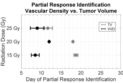
Figure 4. 7 Dose dependence of the early detection of treatment failure by tumor vascular
density. Partial responder identification using vascular density (black) occurred earlier than using tumor volume (gray). With increasing dose, the difference in the time of identification between vascular density and tumor volume decreased. ([*] significant at p < 0.05).
36
No severe adverse health effects or significant weight loss were observed in any of the rats during the entirety of the study. The orientation of the rat during treatment minimized irradiation of the abdominopelvic region, resulting in less toxicity than in our previous studies where the rat was oriented perpendicular to the radiation beam. Mild radiation enteritis was experienced by less than 5 rats which resulted in loose stool and an average of 5 grams or 3% loss of body weight. This was mitigated with supplementary high calorie food and hydrogel water (Methods section). All rats with recurring tumors were euthanized at the end of the study. Rats with successfully treated tumors have been kept indefinitely (>180 days) since the end of the study and have not shown any signs of tumor recurrence.
4.3.ii PN, SOAM, DM, and TCM Results
No significant differences in PN, SOAM, DM, and TCM growth curves were measured between partial responders, complete responders, and untreated controls at any time points. There were no dose dependent differences observed in any of the treatment groups. A summary of the growth curves is presented in Supplementary Figure C.1. There is an average increase in PN measured in the partial responders in all dose groups, however the average trends in PN for complete responders is inconsistent. Tortuosity measurements were compared at time points where VVD and TV clearly showed differences between partial and control responders, however no significant differences were found between groups. These data are summarized in
37 4.4 Discussion and Conclusions
We have previously demonstrated that AA can visualize microvasculature with high-resolution and various quantitative metrics are sensitive to certain abnormal microvascular structural properties (e.g. tortuosity, density) that allow us to discern cancerous tissue from normal tissue [59,60]. Based on previous research that has demonstrated that microvascular remodeling occurs within days after radiation exposure using optical imaging, we hypothesized that quantification of microvascular changes using AA may indicate response to therapy sooner than using TV alone, the current clinical standard for assessing response to treatment [35]. In this work we have demonstrated that quantitative AA is sensitive to changes certain microvascular features induced by RT and its feasibility as a tool for predicting treatment response.
We believe the clinical implications of our data are significant. In this tumor model, we have demonstrated that by quantifying the dynamic microvascular response to RT, tumor recurrence can be detected earlier than using TV measurements alone. In clinical practice, irradiated tumors often do not significantly change in size until 3-4 months after treatment and therefore post-treatment imaging is also not performed during this time [71]. For any cancer patient, early detection of cancer and early assessment of treatment response is critical for
maximizing the chances for improving or maintaining quality of life. By decreasing the wait time between treatment and post-treatment evaluation, we may be able to increase the probability of successfully modifying an unsuccessful treatment strategy to one that is tailored to the patient. This is specifically important for RT, which by itself is often used with radical intent more than in a palliative setting.
38
VVD regrowth associated with tumor recurrence in partial responders occurs significantly sooner than TV regrowth. In the tumors that present complete response, VVD and TV both decrease at similar rates until the tumor completely disappears.
We observe three phases after RT in both the VVD and TV curves, as described by Kozin et al: 1) initial treatment response presented by a continued increase in TV and VVD, 2) tumor regression phase presented by decrease in TV and VVD, and in partial responders, 3) tumor recurrence phase [72]. In the initial treatment response phase we observed an increase in VVD that occurred at a significantly greater rate than in untreated tumors, most likely due to short term inflammation and subsequent hypervascularization caused by the high-dose RT. This observation is supported by previous pre-clinical studies that observed hyperperfusion immediately after RT [30]. Days before TV recurrence (TVx) is measurable in the partial responders, the tumors begin to undergo a rapid increase in VVD which can be visualized on imaging and quantitatively measured. While we do not have data supporting why VVD increases earlier than TV, prior evidence suggests that the tumor endothelium experiences stress induced expression of vascular endothelial growth factor (VEGF) and αvβ3-integrins, therefore evading cell death and possibly promoting revascularization and tumor cell proliferation [73,74].
39
Although a higher VVD at the time of treatment might be associated with an increase in tumor oxygenation and improved RT outcome, this hypothesis remains unanswered with conflicting reported results from previous studies [77]. Hypoxic tumors are known to be more radioresistant than normoxic tumors due to a number of reasons including the lower probability of reactive oxygen species produced by ionizing radiation forming fewer DNA strand breaks as well as the negative effect of hypoxia on the pathway for DNA damage repair resulting in a more
radioresistant cell type [78]. While many previous studies have observed a positive correlation between VVD and therapeutic response, others have reported that VVD has no effect, or an inverse correlation with treatment response [77,79]. We speculate that in this particular tumor model, endothelial cells within the larger tumors, which inherently have a higher VVD, may undergo a smaller fraction of lethal radiation damage than smaller tumors and can eventually repair, possibly encouraging tumor regrowth. Due to the variability in tumor growth rates and unforeseen treatment scheduling complications, our initial size distribution was not comparable in all dose groups and is a confounding factor in explaining the effect of initial VVD on
treatment outcome.
40
We chose to use a simple, single high-dose fraction treatment to demonstrate feasibility of our imaging technique. Our dosage scheme was determined based on pilot study results (unpublished) of a longitudinal RT study performed at 0, 5, and 20 Gy in the same rat and tumor model. In the 20 Gy treatment group, approximately ~50% resulted in complete response. We chose doses between 15 and 25 Gy to investigate the TV and VVD differences between complete responders and partial responders while also determining any dose dependent responses.
Conventional dose fractionation, or the division of the total radiation dose into multiple smaller doses over 7-8 weeks, is clinically used to reduce healthy tissue toxicity by allowing cellular repair in between successive treatments [81]. At this point, the effect of a dose fractionated scenario on tumor VVD is unclear and is an important, clinically relevant question that still needs to be answered. Our high-dose treatment conditions are more relevant to stereotactic body radiotherapy (SBRT) or stereotactic radiosurgery (SRS), and hypo-fractionated RT, which precisely deliver high dose radiation to the target tissue with just a single or few treatments [82]. Hypofractionation and SBRT/SRS, while relatively new and controversial in the field of RT, are promising techniques that may reduce toxicity while improving tumor control [82–84]. The results from this initial study motivate us to conduct further investigation under experimental conditions closer to more clinically relevant applications that incorporate conventional and hypo-fractionated RT.
The microvascular changes observed in this study are specific to the Fisher 344 rat FSA tumor model. Since this tumor strain has been shown to be highly oxygen dependent we made an assumption that areas of hypovascularity (hypoechoic regions) represented necrotic and
41
the hypoechoic regions as necrotic/perinecrotic to validate our analysis. This can be performed in future studies using the TUNEL assay and haemotoxylin and eosin staining [85].
As mentioned previously, tumor hypoxia and necrosis play an important role in tumor response to radiation [17,80]. However, no significant correlation between tumor necrosis and regrowth was observed. The reason for this may be two fold. First, tumor recurrence may not necessarily separate partial from control responders based on malignancy. Rather the data
suggest that initial tumor size likely plays a role in treatment failure. While recurring tumors may develop necrotic regions, complete responding tumors are rapidly dying and exhibit loss in vascularity. Since PN is a fraction of the TV, any necrotic region measured in smaller, regressing tumors may account for a large percentage of the total volume.
Based on the previous studies by Bullitt et al, that demonstrated vascular normalization in response to successful RT response, a similar response trend was expected in our study.
Interestingly, no significant changes in vascular morphology was detected using any of the metrics. The reason for this discrepancy is uncertain, but we suspect that the treatment conditions may have an effect on the microvascular response. The cancer treatment described by Bullitt et al was whole brain radiation [36]. Although treatment details were not shared, whole brain
radiation is typically fractionated by 20-40 Gy/5-10 fractions, limiting a single fraction to 3-4 Gy [86]. This is in contrast to the treatment conditions used in this study which consisted of a single high dose of radiation in the range of 15-25 Gy, in a small rodent model. Revisiting vessel tortuosity changes is warranted with future studies with gentler treatment conditions (i.e. fractionated radiation, 15 Gy/5 doses).
42
patterns, including both avascular (hypoxic) and vascular development [87]. Further
investigation using this technique in different types of human-derived tumor models is warranted since the microvascular response after exposure to radiation will likely vary among different tumor types. Regardless, we are encouraged from these results that quantitative microvascular measurements using AA may significantly improve the current methods for treatment
assessment.
In our study we retrospectively categorized the treated tumors as complete response or failure based on the final treatment outcome. The development of a predictive tool indicating treatment outcome based on repeated VVD (or other vessel morphological features) and TV measurements will be highly relevant to the clinical translation of this diagnostic technique.
43 CHAPTER 5:
Preliminary Functional Principal Components Analysis on Longitudinal Microvascular
Imaging Data Sets
5.1 Overview