A ridge restricted maximum likelihood approach to spatial models

(1)

A Ridge Restricted Maximum Likelihood Approach to Spatial

Models

Brian J. Lopes

A dissertation submitted to the faculty of the University of North Carolina at Chapel Hill in partial fulfillment of the requirements for the degree of Doctor of Philosophy in the Department of Statistics and Operations Research (Statistics).

Chapel Hill 2011

Approved by:

Richard L. Smith

Douglas G. Kelly

Yufeng Liu

Marc L. Serre

(2)

c

2011

(3)

ABSTRACT

BRIAN J. LOPES: A Ridge Restricted Maximum Likelihood Approach to Spatial Models.

(Under the direction of Richard L. Smith.)

Ridge restricted maximum likelihood (RREML) is a new method for regression analysis

in linear models with dependent errors. Assume the linear model where the stochastic error

terms are not independent, and the covariance structure is a function of some covariance

pa-rameter, in this case a spatial covariance parameter. Restricted maximum likelihood (REML)

could be used to estimate this covariance parameter, but REML has no built-in methods for

when multicollinearity exists in the design matrix. RREML takes the Bayesian analog of the

ridge regression model, but modifies the context in order to incorporate the estimation of the

variance parameter. The motivation behind such an approach is that by introducing a bit of

bias in the estimator we will stabilize the variance of the estimates. By weighting the

covari-ance of the prior distribution appropriately, the analysis should be able to both incorporate

the information from the prior distribution and control the influence it has on the posterior

estimates of the model.

This work involves an approach that will be used in order to confront the inherent

multi-collinearity of the design matrix obtained in inverse modeling as discussed in Kasibhatla et al.

(2002). A Bayesian linear regression approach is commonly used in the atmospheric chemistry

community in order to deal with the instability of the linear model, but it is found that these

predetermined prior distributions can be too influential on the final results of the estimates.

The goal of the proposed work is to control this sensitivity to the prior distribution while also

(4)

ACKNOWLEDGEMENTS

I would like to thank everyone who has supported me throughout my studies. Especially

my family who has constantly encouraged me to stay strong. My colleagues I met through

graduate school at UNC have also played a significant role in completing my dissertation. I

treasure each friendship I have made through these years, and consider them all a permanent

part of my life. Lastly, the faculty and staff of the Department of Statistics and Operations

Research, especially my adviser, whose lessons throughout my time in North Carolina are

(5)

List of Tables

4.1 AIC of Site Data . . . 39

4.2 AIC of MOPITT Data . . . 41

4.3 Table of Estimates and Standard Deviations for Site Data . . . 42

4.4 Table of Estimates and Standard Deviations for MOPITT Data . . . 47

4.5 Summary of Exponential Simulation Results . . . 48

4.6 Summary of Gaussian Simulation Results . . . 48

4.7 Comparison of Estimates by MSE . . . 49

4.8 Comparison of 80% Confidence Intervals . . . 49

5.1 X used in simulations . . . 77

6.1 Variance Decomposition ofX5 . . . 95

6.2 Summary of πkj for X’s . . . 95

6.3 Summary of Variance Decomposition ofX∗ in Simulation Setup . . . 102

7.1 Variance Decomposition ofK for Station Data . . . 109

7.2 Variance Decomposition ofK for MOPITT Data . . . 113

7.3 Max. a Posteriori and RREML AICs of Station Data . . . 114

(10)

List of Figures

1.1 Station Locations . . . 6

3.1 Idealized Form of Variogram . . . 23

4.1 A Posteriori Estimates of x for Site Data . . . 40

4.2 A Posteriori Estimates of x for MOPITT Data . . . 40

4.3 All Distances . . . 44

4.4 Minimum Distance per Station . . . 45

5.1 Location of Example Stations . . . 67

5.2 Exponential Derivatives of MSE at 0 . . . 68

5.3 Gaussian Derivative of MSE at 0 . . . 69

5.4 First Exponential Theoretical MSE . . . 70

5.5 Second Exponential Theoretical MSE . . . 71

5.6 First Gaussian Theoretical MSE . . . 72

5.7 Second Gaussian Theoretical MSE . . . 73

5.8 First Simulation of Exponential . . . 74

5.9 Second Simulation of Exponential . . . 74

5.10 First Simulation of Gaussian . . . 75

5.11 Second Simulation of Gaussian . . . 75

5.12 Log MSE of betas for First and Second Exponential . . . 76

5.13 Log MSE of betas for First and Second Gaussian . . . 76

6.1 Spatial Patterns Simulated . . . 93

6.2 Exploring the Asymptotic Properties of the MSE in the Linear Location Case . 97 6.3 Exploring the Asymptotic Properties of the MSE in the Grid Location Case . . 97

6.4 Simulated RREML MSE (Linear on Left, Grid on Right) . . . 99

6.5 Simulated MSE ofβ (Linear on Left, Grid on Right) . . . 100

(11)

6.7 Variance Decomposition Information at λ= 0 for Grid . . . 103

7.1 Station Locations vs. MOPITT Satelite Locations . . . 106

(12)

Chapter 1 Atmospheric Inversion Theory

1.1 Overview

Often scientists face the issue of trying to gauge some element in the world or environment

without having access to a direct or precise measuring instrument. The environmental sciences

must deal with this issue on a regular basis, where the data obtained are actually a function

of a complex physical model used in order to estimate the measurements desired. Whether

the desired data are too expensive to obtain, not easily obtained or are too remote to access,

inverse theory can be a useful alternative in estimating an underlying process or field. The inverse model is a way of incorporating prior knowledge of the system, and relating the

information that can be obtained to estimate the desired state.

Source apportionment is the application of inverse theory by incorporating atmospheric transport models along with observed spatial measurements in order to derive estimates of

sources and sinks of the element being studied. Anatmospheric transport model is a numerical model describing the time-evolution of minor atmospheric constituents in response to

atmo-spheric motions (Enting, 2002). This approach is of particular interest when trying to model

trace-gas or particulate matter. A trace-gas is

A minor constituent of the atmosphere. The most important trace gases con-tributing to the greenhouse effect are water vapor, carbon dioxide, ozone, methane, ammonia, nitric acid, nitrous oxide, ethylene, sulfur dioxide, nitric oxide, dichlo-rofluoromethane or Freon 12, trichlodichlo-rofluoromethane or Freon 11, methyl chloride, carbon monoxide, and carbon tetrachloride. (O’Hara, 1990)

(13)

spatio-temporal distribution. By incorporating these estimates and how an atmospheric

trans-port model can help explain the movement and reactions of the element once released into the

atmosphere, estimates of the original sources (or sinks) contributing to this distribution can

be derived. The general inverse model approach is widely applicable, but necessitates a more

sufficient statistical methodology in many situations. Analyzing the stochastic properties of

the model, estimation of the model and using data assimilation techniques in order to

main-tain model ‘behavior’ are all open areas of research for this approach. One particular issue at

hand is the inevitable fact that these models are often either over- or under-determined. The

need for a more statistical approach in how to deal with this multicollinearity or

overparam-eterization is clear.

The inverse problem is not only used in the environmental context, but can be found in a

vast array of scientific disciplines. One can find applications of this approach in fields such as

medical imaging, astronomy, geophysics and economics . Such broad applicability shows how

useful this approach can be, and how much active research is being published that incorporate

inverse modeling. There are even journals focused entirely on the discipline, such asInverse Problems by the Institute of Physics, theJournal of Inverse and Ill-posed Problems from VSP International Science Publishers, and Inverse Problems in Science and Engineering from the Taylor & Francis Group.

1.2 General Inversion Model

Along with the many journal articles available on inverse problems, there are also many books

that cover the topic extensively. Tarantola (2005), Enting (2002) and Rodgers (2000) are all

comprehensive references on the topic. In this section the generalized mathematical inverse

model will be discussed, as well as the two main applications of this model.

When describing an element’s contributive sources, it is useful to look at the rate of change

of the concentrations with respect to time. Ifm(~r, t) is the concentration at timetand spatial location~r, then

∂

(14)

for a current concentration is the sum of the source at the location plus any contribution due

to the transport from the concentrations at other locations. There are two main classes of

inversion models used in practice, a ‘differential’ version that uses a slightly modified version

of (1.1), and an ‘integral’ model that uses Green’s functions. Beyond these two approaches

there are many other hybrid models as well (Enting, 2002).

1.3 Differential Inversion

The differential inversion method is often referred to as the mass-balance technique as well.

In order to use this approach, rearrange (1.1) as

b

s(~r, t) = ∂

∂tmb(~r, t)− T[mb(~r, t), t], (1.2)

where the hat denotes statistical estimates of the parameters and functions. Specifically,

b

m(~r, t) is a statistically smoothed estimate of the observed concentration fieldc(~r, t). Often (1.2) is used to derive surface sources, wherein (1.1) is used to integrate throughout the free

atmosphere (Enting, 2002).

1.3.1 Forward Model Approach

Rodgers (2000) discusses an application of the Differential Inversion approach in order to

get a linear approximation. The final model leads to the traditional least-squares model in

Statistics, as can be seen in the work done in Kasibhatla et al. (2002). The work proposed

throughout this document will be focusing on this model. Consider a vector of the observable

measurements one can take, call thisy~I, and the unknown variables of interest describing the

state space in a (p×1) vector~x. For each state vector, there is an ideal measurement vector ~

yI which can be described by theforward function,f(~x), such that

~

yI =f(~x).

The forward function is determined by the physical properties behind the measurements and

(15)

element throughout the environment onto the space measured by y~I. Yet because this is an

idealized relationship, and f(~x) is not easily determined, reality forces the use of a forward model,F(~x) as an approximation of the true physics and chemistry involved in f. Typically, one is limited to a finite number of measurements and locations, leading to an (n×1) vector of measurements,~y. Hence, the relationship would be

~

y=F(~x) +, (1.3)

where is a stochastic error term. Now by using (1.3) the model can be linearized around some reference point~x0 by taking the Taylor expansion about ~x to get

~

y−F(~x0) =

∂F(~x)

∂~x (~x−~x0) +=K(~x−~x0) +. (1.4)

K is the (n×p) matrix known as the kernel or Jacobian, with element (i×j), Ki,j =

∂Fi(~x)/∂xj. The current application of this approach setsx~0 =~0, and assumes thatF(~0) =~0.

Applying these assumptions leads to the final model

y=Kx+. (1.5)

While (1.5) can be looked at as a typical ordinary least squares model what is not seen here is

the typical multicollinearity ofK. The atmospheric chemistry community often use a Bayesian linear regression approach to (1.5) in order to deal with this numerical instability. When using

the Bayesian framework, it could be argued that using any prior distribution without mean~0 could be counter-intuitive to the Taylor expansion employed in the forward model approach.

While this point is being acknowledged here, it is considered beyond the scope of the current

work, because the model has been predetermined by the work of Kasibhatla et al. (2002).

The process of obtaining theK used in the forward model is quite involved. The purpose of K is to describe the sensitivity of the measurement vector to finite changes in the state vector (Arellano Jr, 2005). Based upon the context of the problem, a numerical modeling

system of the transport model is chosen. These algorithms will typically take a set of starting

(16)

After monitoring the change in the initial values, the components of the design matrix K can be found. It is possible for the modeler to incorporate the spatial and temporal correlations

along with the physical, chemical and biological properties involved in the environmental

process. Of particular interest in this derivation are the numerical issues involved with the

use of this matrix operator. Often these partial differential equations lead to ill-conditioned

or even singular K matrices. The current approach discussed in this dissertation will not account for the stochastic properties involved with the estimation of K, but instead to treat this as a fixed and known matrix.

1.4 Source Apportionment of Carbon Monoxide

Carbon monoxide (CO) is a trace gas produced from the incomplete combustion of carbon

fuels as a by-product during the oxidation of carbon containing compounds in the atmosphere

(Arellano Jr, 2005). Understanding this gas is important not only due to its major short-term

health implications, but also because it can help explain the overall chemical system in the

troposphere. CO is known to be a major chemical sink or source for numerous chemically

and radiatively important trace species including several greenhouse gases (Arellano Jr, 2005).

The main sources of carbon monoxide are from anthropogenic sources such as automobiles,

industrial activity, heating and the burning of agricultural waste products. By getting a better

understanding of the sources of this trace gas, environmental chemists hope to get a better

signal related to human impact on the atmospheric chemistry picture.

The inverse problem has become a useful tool in analyzing sources in atmospheric

chem-istry. Kasibhatla et al. (2002) used this approach, in which they used a “top-down” approach in

order to estimate the various sources of carbon monoxide in disaggregated regions throughout

the world. The “top-down” approach is to use the surface measurements of carbon monoxide

(CO) levels from various global monitors, and use the Jacobian of an atmospheric transport

model in order to relate the observed levels to the various sources of the gas. After solving

the resulting inverse problem, they compared the results with the traditional “bottom-up”

estimates, where large discrepancies between the two approaches were found. The direct or

(17)

contributions from different human or natural resources based upon documented records or

land surveys.

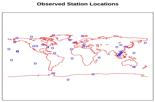
Figure 1.1: Station Locations

Observed Station Locations

o o

o

o o

o _o _o

o o

o

o o

o

oo

o _o

o

oooooo o

o o

o

The details of the forward model are outlined in (Sec. 1.3.1), with the general formula given

in (1.5). Before defining the variables used in (1.5) it is necessary to describe the chosen data

for the surface CO measurements. The NOAA/CMDL Cooperative Air Sampling Network

(Novelli et al., 1998) provides time series of CO mixing ratios for various stations located

throughout the globe, and can be obtained from http://www.cmdl.noaa.gov/ccgg/index.

html. Of particular concern with the series associated with each measurement station is that

the observations are not on a regular temporal schedule, and each station has its own set of

missing values. Therefore, Kasibhatla et al. (2002) mirrors the approach discussed in Novelli

et al. (1998) when dealing with such data. For most sites the series of CO measurements

start between 1989 and 1992, with six stations not starting to record values until 1993/1994,

but all series extend through 1996 (Kasibhatla et al., 2002). When looking to define surface

(18)

when looking at a station. Thus when looking at the series for each site, the monthly mean

concentrations for 1994 are derived from the multi-year CO measurements using the smoothing

method discussed in Novelli et al. (1998). These monthly measurements will be used in the

vectory as the monthly CO concentrations for each station.

In order to account for the errors of y, Kasibhatla et al. (2002) used the root mean square of the individual series measurements from a specified month with the mean being treated as

the monthly-mean defined iny. In order to avoid bias due to the sparsity of the data within a given month, only months in which there were at least 3 measurements over the period

1993-1995 were considered in this analysis, and any sites with less than 7 months of statistics is

removed from the overall analysis (Kasibhatla et al., 2002). Whenever it applied, a minimum

root mean square threshold of 20% for background sites, and 30% for source sites, was used

when accounting for the error values ofy. Based upon these criteria for selecting stations and months, there are 38 stations used as seen in (Fig. 1.1), and 419 observations in y.

K is the (n×p) Jacobian matrix of the global chemical transport forward model provided by the Atmospheric Chemistry Modeling Group at Harvard University (2005), which is a

function of the states. This transport model was run at a resolution of 4◦ ×5◦, with both

temporal and spatial patterns prescribed in the forward model. The reader is encouraged to

refer to Kasibhatla et al. (2002) for the prescribed details when running the model in this

analysis. Essentially, the authors based their belief of starting values and their transport

based upon previous research and recorded data, and these are incorporated in the forward

model.

x is the (p×1) state vector for the 12 month average emissions for various anthropogenic sources and regions. These can be broken down to:

• FF/BF-NA, FF/BF-EU, FF/BF-AS and FF/BF-RW represent the fossil-fuel/biofuel

consumption sources in North America, Europe, Asia and the Rest of the World,

re-spectively.

• BB-NA/EU, BB-AS, BB-AF, BB-LA and BB-OC represent the biomass-burning sources

in North America/Europe, Asia, Africa, Latin America and Oceania, respectively.

(19)

• METH represents the CO yield from methane (CH4) oxidation.

Each of these will be assigned tox1, . . . , x12, respectively.

Lastly,is the vector of errors (possibly heterogeneous), but initially assumed independent in Kasibhatla et al. (2002) due to the fact that both temporal and spatial interaction was

prescribed in the forward model. There aren= 419 station observations over the 12 months, and these are being mapped ontop= 12 contributive sources/sinks.

A Bayesian framework was used in order to calculate the “top-down” estimates with the

above data. Assume that

p(y|x, S, K)∼N(Kx, S)

with S assumed known, and to be a diagonal matrix of the root means squares. The prior

distribution of x is x ∼ N(xa, Sa), where xa is obtained from the “bottom-up” estimates as

discussed in Kasibhatla et al. (2002), and the diagonal of Sa is set to be half of xa. Recall

that the inventory method used in xa is an estimate of each regions contributions, and lack

any measurement of the potential error involved. Therefore, a moderate variance was chosen

to be used in the prior covariance. Again,Sa is also set to be of diagonal (independent) form.

Based upon these assumptions, estimating x giveny in (4.1) gives:

x|y∼N(x,b Sb),

where

b

x=xa+G(y−Kxa),

withGbeing commonly referred to as the gain matrix, defined as

G= (KTS−1K+S_a−1)−1KTS−1.

The posterior covariance is then defined as

b

S = (KTS−1K+S_a−1)−1.

(20)

ap-proach. Of primary concern to the authors was the need to account for any spatial correlation

in the estimates. While the choice of using Bayesian least-squares regression is a justified one

in dealing with the potentially ill-conditioned matrix, K, there is an opportunity to explore other statistical approaches to this model. Initial attempts at enhancing this approach will

be adding a spatial covariance to the analysis with the eventual goal to be able to also

con-trol for the influence the prior distribution has on the posterior estimates of both the spatial

(21)

Chapter 2 Linear Model Theory

Linear models are common when performing a statistical analysis of scientific data. Although

ordinary least squares regression (OLS) is one of the more popular approaches in basic

statis-tical analysis, scientists may encounter data where alternative methods should be explored.

Ill-conditioned problems expose weaknesses in the OLS approach where parameter estimates

often have large variances, false model assumptions are often magnified, and even algorithm

issues become a problem. Often one can try to reduce the factors in the design matrix so as

to avoid such strong interaction within the covariates. Recall the forward model described in

(Sec. 1.3.1), where the physics behind the model are what dictate the design matrix, thus

the options are limited when dealing with the inherent multicollinearity. Removing any of the

covariates would drastically affect any scientific interpretation of the results.

There is a vast amount of literature on various approaches that parallel OLS, but deal

with some of these modelling issues directly. The class of regularized estimators is a set of

approaches in which one tries to confront multicollinearity. The term regularized emanates

from the method of regularization in approximation theory (Brown, 1993).

2.1 Ordinary Least-Squares

The linear regression model can be written as

(22)

withY being ann×1 vector of observed responses,X then×(p+1) design matrix of recorded covariates for each of the observed responses, θ = (µ, βT)T a (p+ 1)×1 vector of unknown parameters with the first column being a vector of 1, and is the n×1 vector of random errors. Typical second-order assumptions treat∼ N(~0, σ2I), as well as havingindependent of the observed covariates. Thus the mean for each observedYi would beE(Yi|xi) =µ+xTi β.

The ordinary least-squares approach is to find an estimatorθbthat minimizes the residual sum

of squares

(Y − Xθb)T(Y − Xθb),

which is a solution to the ’normal’ equations

XTXθb=XTY.

Assuming that X is of full rank, the OLS estimator is

b

θ= (XTX)−1XTY.

Recall that if two multivariate normal random vectors are orthogonal, then they are

inde-pendent. This independence can be exploited when exploring the distributions of the intercept

and slope terms in (2.1). By centering the covariates such that

X

i

xij = 0, j = 1, . . . , p, (2.2)

independence between the intercept and covariance terms will be forced. This is seen more

clearly when looking at (2.1) with a slightly different parametrization

Y =µ†~1 +Xβ+, (2.3)

with µ†=µ+P

jβjx¯j. Without loss of generality (WLOG), linear models will be assumed

(23)

X†= (~1, X) the OLS estimate for (2.3) is

b

θ†= (X†TX†)−1X†TY. (2.4)

2.2 Regularized Multiple Regression

Ordinary least squares estimates are known to be the best linear unbiased estimators (BLUE)

for the linear model. However, it is possible to find some biased estimators that may have

smaller mean-squared error (MSE). One such example is the ridge estimator. This can

espe-cially be the case when the design matrix is nearly singular or ill-conditioned, in which case

it can be debated as to which approach is appropriate for the given context. These

alterna-tive estimators are sometimes referred to as regularized estimators or shrinkage estimators,

because they reduce the estimated parameters compared to that of OLS (Brown, 1993).

Ridge regression (RR), principal components regression (PCR), partial least-squares

re-gression (PLSR) and minimum length least-squares (MLLS) are all commonly used

regular-ization techniques. All of these regularized estimators can be looked at as

b

βR=GXTY, (2.5)

or

b

YR=µb+HY, (2.6)

whereH=XGXT. Comparing this with the OLS estimator of (XTX)−1XTY, shows thatG

is just an approximation of the ‘inverse’ ofXTX. Ridge regression takes

G= (XTX+_bcIp)−1, (2.7)

(24)

Principal components regression starts from the spectral decomposition

XTX=

p

X

j=1

λjvjvjT,

so that

G= X

j∈Sw

(1/λj)vjvjT. (2.8)

Sw is a subset ofw ≤min(p, n−1) indices of thepvariables chosen by one of the two methods:

1. decomposition of variance based on eigenvalues ofXTX,

2. those eigenvectors for which the correlation withY is high,

with the former being traditional PCR, and the latter being a hybrid version (Brown, 1993).

PLSR inverts using a conjugate gradient algorithm for matrix inversion. MLLS is a

special case of all three of these regularization techniques, corresponding to the Moore-Penrose

generalized inverse of (XTX) (Brown, 1993).

The motivation for using regularized estimators is to introduce bias in order to reduce

variance. Ideally, this overall effect can help reduce the risk, or expected loss, of the estimator.

Within the quadratic loss framework, the risk function is usually considered as

R(βb_R, β) =E

(βb_R−β)TL(βb_R−β)

. (2.9)

L = Ip and L = XTX are popular choices, corresponding to estimation mean-squared and

prediction mean-squared error, respectively (Brown, 1993). Another possibility would be to

use a different design, X2 for prediction, and use L = X2TX2. Keep in mind that

predic-tion at model points is more accurate than predicpredic-tion or estimapredic-tion in direcpredic-tions with small

eigenvalues.

The background of the model in the work described in (Sec. 1.3.1) implies the need to

take care to preserve the interpretative values of the design matrix. In order to account for

the numerical instability, the work in Kasibhatla et al. (2002) took a Bayesian approach,

which under the appropriate conditions mirrors RR. Expanding on the work in (Sec. 1.4)

(25)

prior distribution used in Kasibhatla et al. (2002).

2.3 Ridge Regression

Although Hoerl and Kennard (1970a) and Hoerl and Kennard (1970b) are said to have

popu-larized the idea of adding a constant to the diagonal ofXTX, the method was first suggested in Hoerl (1962). Ridge estimators are closely allied to Bayes estimators, and because of this

gain some statistical admissibility.

Algorithm 2.3.1. The recipe given by Hoerl and Kennard (1970a) and Hoerl and Kennard

(1970b) is as follows. If there is a model of the general form (2.3)

1. Scale the p x-variables so that the diagonal elements of XTX are n (some approaches set the matrix to be of correlation form with diagonals of 1).

2. Plot the components ofβb_RR(c) versusc, where

b

βRR(c) = (XTX+cIp)−1XTY. (2.10)

This is often called the ridge trace. Note that the estimator ofµis often taken to be ¯y, irrespective ofc.

3. Plot the residual sum of squares as a function ofc on the ridge trace diagram.

4. Choose the value of_bc which stabilizes the coefficient trace, and minimizes the residual sum of squares penalty.

Because this approach relies heavily on visual inspection of the trace diagram, it is often

criticized for its ease of misinterpretation (Smith, 1980). In cases of ill-conditioned, near

collinear problems, dramatic changes to the coefficient estimates may be seen in the ridge

trace diagram. Keep in mind that the scaling of the diagonal of XTX is different from the ‘correlation’ form when described in Brown (1993), although Hoerl and Kennard (1970a) and

(26)

2.3.1 Benefits and Comparison

Hoerl and Kennard (1970a) and Hoerl and Kennard (1970b) also outlined the benefits of using

ridge regression over ordinary least-squares regression. The beneficial effects of using (2.10)

are more easily seen when taking the singular value decomposition (SVD) ofX in (2.3). The use of the SVD not only assists with the numerical stability of the problem, it is also a useful

aid in understanding the derivation of the properties for both the RR and OLS estimators.

Before sketching this out, it is helpful to be familiar with the SVD of a matrix. Briefly, for an

(n×p) matrixX, let t= min(n, p) and set the matrices T to be (n×t) andV to be (p×t), then

X=T DVT, (2.11)

whereDis a (t×t) diagonal matrix of the ordered singular values,di (1≤i≤t) of the matrix

X. That is, d1 ≥ d2. . . , dt ≥ 0, and the r ≤ t non-zero values di squared are the non-zero

eigenvalues of bothXTX and XXT. Columns ofT are eigenvectors (orthonormal) ofXXT, and the columns ofV are eigenvectors (orthonormal) of XTX, hence TTT =VTV =It.

In order to compare the benefit of using (2.10) over (2.4) the singular value decomposition

is taken of the regression matrixX, assuming that rank(X) =r≤min(n−1, p). Then taking the matrix product ofTT and (2.3), remembering thatV VT =Ip, to get

U =TTY =TT~1nµ†+TTXV VTβ+TT.

(27)

Now settingVTβ =α gives

U =TTY = TT~1nµ†+TTXV VTβ+TT

= ~0 +TTXV α+TT = Dα+,

whereD is as defined in the singular value decomposition. From this follows

Ui =

  

 

αi √

λi+i, i= 1, . . . , r

i, i=r+ 1, . . . , n−1,

(2.12)

where λ1 ≥ . . . ≥ λr > 0 are the non-zero eigenvalues corresponding to the singular values

described earlier. Thus, the ridge estimator is defined as

b

αiRR=Ui

p

λi/(λi+c), (2.13)

as compared to the OLS estimator

b αiOLS =

  

 

Ui/ √

λi, i= 1, . . . , pnon-zero eigenvalues

indeterminate, zero eigenvalues

(2.14)

Based upon the results from (2.14) it is easy to see how very small eigenvalues can cause the

least-squares estimate to blow up. Yet, the ridge component, c can help to stabilize the case where the design matrix is ill-conditioned, and removing a covariate is not an option. The

direct comparison of the two estimators gives us

b

αiRR={λi/(λi+c)}αbiOLS. (2.15)

(2.15) shows that for c > 0, α_bRR is actually the OLS estimate, αbOLS, shrunken towards

zero. Noticec has a greater effect on components with smaller eigenvalues,λi. These small

(28)

E αb

T

b

α=αTα+σ2X(1/λi).

2.3.2 Ridge Properties

The properties of the ridge estimator go beyond the point estimate itself. The statistic

dis-cussed in (2.15) is in fact biased,

E(αbiRR−αi) =λiαi/(λi+c)−αi =−cαi/(λi+c),

with variance

{λi/(λi+c)}2σ2/λi =λiσ2/(λi+c)2.

In order to explore the potential of this approach, it is useful to look at either the mean-squared

error, MSE, or mean-squared prediction error, MSPE.

E

p

X

i=1

Li(αbiRR−αi)

2

!

=σ2

p

X

i=1

Liλi

(λi+c)2

+c2

p

X

i=1

Liα2i

(λi+c)2

, (2.16)

where Li = 1 corresponds to the MSE, andLi =λi the MSPE. This holds with singularities

(λi = 0) as well. The MSE for the ridge estimate will decrease as c is increased by small

increments from 0.

2.3.3 Determining c in Ridge Regression

As pointed out earlier, the ridge trace diagram leaves much to be desired due to its potential

ambiguity in interpretation. While in principle there exists an optimalcto minimize the MSE, it can not be calculated in practice. There are various techniques proposed to estimate c in practice, and this section will briefly explore the methods used when allowing for a singular

(29)

1. Cross validation estimate, _bcCV is applicable when the data are scaled as described in

(Alg. 2.3.1). Choose cto minimize

||(I−A(c))y||2

[trace(I−A(c))]2, (2.17)

hereA(c) =X(XTX+cI)−1XT.

2. “Automatic” estimates, such as modifying the Hoerl-Kennard estimate with Stein’s or-thogonal case:

b

cM HKB =

(r−2)_bσ2 b

βT_β_b , (2.18)

as well as the Lawless and Wang (1976) estimator

b

cM LW =

(r−2)σ_b2_trace(_XT_X₎

rβbTXTXβb

= (r−2)σb

2_trace(_XT_X₎

rby

T

b

y . (2.19)

3. Minimum unbiased risk estimator, find the_bcM U R to minimize the unbiased estimator of

the risk in (2.16) withLi = 1 (0 whenµi is inestimable)

b

σ2X λi−c λi(λi+c)

+c2X bµ

2

i

(λi+c)2

. (2.20)

4. “type II MLE method”is a universally appealing alternative, as discussed in Lindley and Smith (1972), although its drawback is the potential numerical calculations involved.

Consider the hypothetical two-stage model

β ∼ N(0, σ2/c),

b

β|β ∼ N(β,(XTX)−1σ2). (2.21)

This Bayesian approach leads to the natural approach of using the mean of the posterior

distribution ofβ|βb, which is conveniently the ridge estimator,βb_RR(c). A convenient way

of looking at this would be

b

(30)

which gives the distribution

b

β ∼ N(0, σ2(1/c+ (XTX)−1).

Numerical techniques must be used to find the maximum likelihood estimates for c and σ2, because there is not an analytical solution to the above distribution. Note the Bayesian perspective of this approach, and its similarity with the work discussed in (Sec.

1.4). This is further motivation to explore the RR approach to control for the influence

of the prior distribution in Kasibhatla et al. (2002). Since the type II MLE approach

is derived from a well-specified framework, it appears as a more general approach than

the other methods for determiningcin ridge regression.

2.3.4 Admissibility Based Upon the Bayesian Analog

It is said that an estimateβb_Rdominates another estimator, sayβb, with respect to a particular

loss function if the expected loss is no larger than that of βb for all points in the parameter

space forβ, and strictly smaller for at least one point in the parameter space. Any estimator that is dominated by another estimator is inadmissible. When determining if an estimator

is admissible, it is useful to keep in mind that all proper Bayes estimators (estimators that

minimize the posterior expected loss with a proper prior) are admissible for whatever loss

function chosen (Casella and Berger, 1990).

A motivating factor behind Ridge Regression is its similarities with the Bayesian approach

to linear regression. This analogy solidifies the admissibility of such an estimator. A prior

distribution is put on β that is multivariate normal with mean zero and a known diagonal covariance matrix,σ_β2I, and give the intercept term, µ, an improper a priori distribution that is uniform over the real line and independent from β. Thus, looking at the model described in (2.3) gives

(31)

Settingc= σ_σ22

β

gives the joint posterior distribution

π(µ, β|Y) ∝ exp{− 1

2σ2(Y −µ~1−Xβ)

T₍_Y ₋_µ~₁₋_Xβ₎₋ 1

2σ2_β(β−~0)

T₍_β₋_~₀₎_}

= exp{(YTY −YTµ~1−YTXβ−µ~1TY +µ2~1T~1 +µ~1TXβ−βTXTY +µβTXT~1 +βTXTXβ)− 1

2σ_β2β

T_β_}

= exp{− 1

2σ2(−µY

T_~₁₋_µ~₁T_Y ₊_µ2_~₁T_~_{1 +}_µ~₁T_Xβ₊_µβT_XT_~₁_}

×exp{− 1

2σ2(Y

T_Y ₋_YT_Xβ₋_βT_XT_Y ₊_βT_XT_Xβ₎₋ 1

2σ_β2β

T_β_}

= exp{− n

2σ2(−µY¯ −µY¯ +µ 2₎_}

×exp{− 1

2σ2(Y

T_Y ₋_YT_XIβ₋_βT_IXT_Y ₊_βT_XT_Xβ_{) +}_cβT_β_}

∝ exp{− n

2σ2(µ

2₋₂_µ_Y_¯ _{+ ¯}_Y2₎_}

×exp{− 1

2σ2(Y

T_X₍_XT_X₊_cI₎−1_XT_Y ₋_YT_XIβ₋_βT_IXT_Y ₊_βT_XT_Xβ_{) +}_cβT_Iβ_}

= exp{− n

2σ2(µ−Y¯)

2_{} ×}_exp_{− 1

2σ2(β−βbRR(c))

T_W₍_β₋

b

βRR(c))}.

Hereβb_RR(c) is defined as in (2.10), and

W = (XTX+cI).

From this derivation it can be seen that the joint posterior distribution is the product of two

independent distributions for bothµand β, where

µ|Y ∼N( ¯Y , σ2/n),

and

β|Y ∼N(βb_RR(c), σ2W−1). (2.23)

Recall that under squared error loss the posterior mean is the Bayes estimator, therefore the

ridge estimator is the Bayes solution under the conditions stated above, and hence admissible.

(32)

Chapter 3 Linear Models with Unknown Covariances

In spatial statistics it is common to deal with observations that have some form of correlation

involved. A typical approach to such models is to fit the covariance to some parametric form

that is a function of a few parameters, usually denotedθ. In cases such as this, Cov(Y, YT) = V(θ) when looking at the model in (2.3), andV(θ) is no longer considered a diagonal matrix. Now the approach chosen by the researcher must be concerned with choosing the parametric

form ofV(θ) along with estimating the parameters of bothβ andθ.

3.1 Spatial Processes and Variograms

This section will provide a quick overview of spatial processes and the variogram, and the

various assumptions that come into play when using them. This is a brief synopsis of the

information provided in Smith (2001). Assume there is a stochastic process {(s) :s ∈D}, in some space D. There are some fundamental properties and definitions of spatial processes necessary to discuss in order fully to understand the proposed work.

• The process isGaussian, if the joint distribution of ((s1), (s2), ..., (sk)) for any points

s1, s2, ..., sk∈D is multivariate normal.

• The process is called strictly stationary if for any points s1, s2, ..., sk ∈ D and h then

((s1), (s2), ..., (sk)) and ((s1 +h), (s2 +h), ..., (sk +h)) have the same joint

(33)

• The process is said to beweakly stationary (orsecond-order stationary) if:

– µ(s) =E[(s)] =µfor all s∈D, and

– Cov[(s1), (s2)] =C(s1−s2) for any two points s1, s2 ∈ D. In other words, the

covariance only depends on the distance and direction of the two points, not on

their specific locations.

• A process isintrinsically stationary if

– µ(s) is a constant for alls∈D, (call this 0 WLOG).

– The variance of the difference can be defined as

Var[(s1)−(s2)] = 2γ(s1−s2), (3.1)

where this makes sense if the variance of the difference of the two ’s only depends on the difference s1 −s2. The function 2γ(·) is called the variogram, and γ(·) is called

the semivariogram. It is easily shown that if a process is weakly stationary, then it is intrinsically stationary, but not conversely.

• A process isisotropic if the process is intrinsically stationary and the semivariogram in (3.1) can be written as

γ(h) =γ0(||h||), (3.2)

for some functionγ0. Here the semivariogram only depends onh through ||h||, or only

the distance between the two sites. It may help to think of||h|| asd, which is just the distance between the two locations. It is possible to estimate the parameters that define

this functionγ0.

• If a process is both intrinsically stationary and isotropic, then it is calledhomogeneous.

From these definitions, some very useful properties can be applied, and proven in a trivial

manner. The proof of these results will be left up to the reader.

• If the process is weakly stationary, then a convenient way to look at the semivariogram

is

(34)

whereC(·) denotes the covariance. Thus, ifC(h)→0 ash→ ∞, then this formula can be used to findC(0).

• If the process is both Gaussian and weakly stationary, then it is strictly stationary.

• If all of the variances are finite, then a strictly stationary process is also weakly

station-ary.

• If limh0_→∞γ(h0) is finite for an intrinsically stationary process, then the process is weakly

stationary as well, and

C(h) = lim

h0_→∞γ(h

0

)−γ(h). (3.3)

3.2 The Semivariogram

γ

0

(

· )

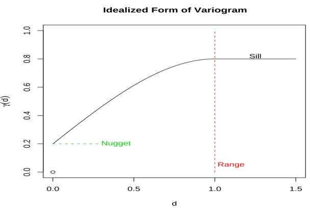
Figure 3.1: Idealized Form of Variogram

0.0 0.5 1.0 1.5

0.0

0.2

0.4

0.6

0.8

1.0

Idealized Form of Variogram

d

γ

(

d

)

●

Range

Nugget

Sill

Many of the common parametric forms of the semivariogram are plotted similarly to that

(35)

However, it is not required that this is the limiting value as ||h|| ↓0 or d↓ 0. This limiting value is referred to as the nugget of the semivariogram. Another aspect of the semivariogram

is the sill, which is the limiting value ofγ0(d) asd→ ∞. Note that in some parametric forms

of the semivariogram, the sill is attained at a finite value ofd, and this point is referred to as the range of the semivariogram. The range is defined as the point where the semivariogram

is within a specified distance from its sill. The nugget is an odd phenomenon when looking

at the semivariogram, because it implies some discontinuity in the spatial covariances. There

are many explanations as to the existence of the nugget, one being that it exists due to excess

white noise that may exist over the spatial process. When fitting spatial covariance models,

it is a good idea to explore the fact that there may be no nugget. If this is the case, then all

parameters that involve estimation of the nugget should be removed.

For now, this section will focus on two parametric forms of the variogram γ0(d); the

Ex-ponential, and the Gaussian, and one parametric form of a spacial covariance, the Mat´ern.

While this list is by no means an exhaustive one, it is sufficient for the current discussion.

Further documentation on spatial covariances used in the R package, spatrr, and some

ad-ditional calculations of the covariances defined from the semivariograms discussed in Smith

(2001), see Appendix B. Each of these three spatial parametric models will now be defined,

and discussed in relation to the measurements located at two different sites or stations.

3.2.1 Exponential with Nugget Effect

The exponential semivariogram is defined as:

γ0(d) =

  

 

0 ifd= 0

c0+c1(1−e−d/R) ifd >0.

(3.4)

Using (3.3), the covariance between stations can be calculated as

C0(d) =

  

 

c0+c1 ifd= 0

(36)

If each station has the same known variance,σ2then the covariances can be defined by setting θ= (φ, R) to be the parameters describing the spatial correlations where φ=c0/(c0+c1) is

the nugget:sill ratio parameter, and R is the range parameter, and c0+c1 =σ2. Now define

the covariances as

C0(d) =

  

 

σ2 ifd= 0 σ2(1−φ)e−d/R ifd >0.

3.2.2 Gaussian with Nugget Effect

The Gaussian semivariogram is defined as:

γ0(h) =

  

 

0 ifd= 0

c0+c1(1−e−d

2_/R2

) ifd >0.

(3.5)

Again, by following (3.3) the covariance is defined as follows

C0(d) =

  

 

c0+c1 ifd= 0

c1e−d

2_/R2

ifd >0,

and following the definitions outlined for the Exponential covariance leads to

C0(d) =

  

 

σ2 ifd= 0 σ2(1−φ)e−d2/R2 ifd >0.

3.2.3 Mat´ern

This parametric form is best described by the covariance (assuming isotropy). ThusC(h) = C0(||h||) where,

C0(d) =

  

 

1 ifd= 0

1 2θ₂−1_Γ(_θ

2)

2√θ2d

θ1

θ2

K_θ₂2

√

θ2d

θ1

ifd >0.

(3.6)

Here θ1 > 0 is the spatial scale parameter, and θ2 > 0 is the shape parameter, and Γ(u) =

R∞

0 t

u−1_e−t_dt _{(known as the gamma function) and} _K

(37)

Mat´ern encompasses both the Gaussian and Exponential models. When θ2 → ∞ the Mat´ern

is equivalent to the Gaussian, and ifθ2= 1₂ the Mat´ern is equivalent to the exponential.

Again, the reader should refer to Appendix B for the calculations involved, as well as the

definition of alternative parametric forms of spatial covariance.

3.3 Maximum Likelihood of Spatial Processes

When the spatial process is Gaussian, it is straightforward to write down the exact likelihood

function and hence maximize it. This section will briefly outline the approach described in

Smith (2001) and Mardia and Marshall (1984). Evaluating the likelihood requires the inverse

and determinant of the covariance matrix. It is important to remember that if there are n observations, then the algorithm must invert ann×nmatrix. Asngets larger more computing resources will be necessary in order to perform this evaluation. If∼ N(Xβ,Σ) withXbeing an n×q known matrix of full rank with q < n,β a vector of unknown covariates, and Σ the unknown covariance matrix of the observations. It is often assumed that

Σ =αV(θ), (3.7)

where α is an unknown scale parameter and V(θ) is a vector of standardized covariances. Refer to the covariances defined in the previous section in order to fill outV(θ). The negative log likelihood ofis

`(β, α, θ) = n

2log(2π) + n

2log(α) + 1

2log|V(θ)|+ 1

2α(−Xβ)

T_V₍_θ₎−1₍₋_Xβ₎_. _(3.8)

Note that ifβbis defined as βb= (XTV−1X)−1XTV−1(the GLS estimator ofβ) then

(−Xβ)TV−1(−Xβ) = (−Xβb+Xβb−Xβ)TV−1(−Xβb+Xβb−Xβ)

(38)

which concludes that βb is the choice of β that minimizes (3.8). Keep in mind that V is a

matrix function of θ, and defining

G2 = (−βb)TV−1(−βb),

gives

`(βb(θ), α, θ) = n

2log(2π) + n

2logα+ 1

2log|V(θ)|+ 1 2αG

2₍_θ₎_. _(3.9)

The modeler then has the choice of minimizing (3.9) with respect to α and θ, or to define

b

α(θ) = G

2₍_θ₎

n ,

which will analytically minimize (3.9) with respect toα. Pluggingαb into (3.9) leaves

`∗(θ) = `(βb(θ),α_b(θ), θ)

= n

2 log(2π) + n 2log

G2(θ) n +

1

2log|V(θ)|+ n

2, (3.10)

which is only a function of θ, often referred to as the profile negative log likelihood. This can then be numerically optimized in order to determine the MLE of θ. Keep in mind that there are a few ways to minimize the computational burden of this method, such as using

the Cholesky decomposition before taking the inverse of V(θ), and using a quasi-Newton algorithm in order to get the Hessian at the optimal value.

3.4 Restricted Maximum Likelihood

It is a well known issue that maximum likelihood estimates need not be unbiased. The

pedagogical example is the Gaussian distribution with unknown mean and variance. The

maximum likelihood estimate for the variance of the distribution is biased, and hence not

the BLUE estimator. One answer to such a problem is the Restricted Maximum Likelihood

(39)

Suppose the following multidimensional distribution

Y ∼ N(Xβ, V(θ)),

where the covariances are explained by the parameters inθ. The corresponding negative log likelihood is

l(β, θ) = n

2log(2π) + 1

2log|V(θ)|+ 1

2(Y −Xβ)

T_V₍_θ₎−1₍_Y ₋_Xβ₎_.

Following the approach outlined in Smith (2001), set HT = (XTV−1X)−1XTV−1. This leads to the generalized least squares estimator (with known covariance matrixV),βb=HY.

Then set W = ATY where W is the vector of n−q linearly independent contrasts. It can be shown that A can be chosen such that AAT = I −X(XTX)−1XT and ATA = I. Then if B = [A|H], where B is a partitioned matrix comprised of A and H, the negative log likelihood for W = ATY can be derived by looking first at the likelihood of W† = BTY = [YT_{A, Y}T_H_]T _{= [}_WT_,

b

βT_]T_{, and integrating out}

b

β, following the work in (Harville, 1974), where the similarities between the REML proposed in Patterson and Thompson (1971) and

a Bayesian linear regression approach to the model are discussed.

A brief summary of the work provided in Harville (1974) follows. In order to explore the

distribution ofW†the Jacobian of the transformation fromY needs to be calculated. In which case, it is useful to recall the properties for calculating the determinant of a block matrix.

|B| = |BTB|1/2

=



 

ATA ATH HTA HTH



 

1/2

= |ATA|1/2_|_HT_H₋_HT_A₍_AT_A₎−1_AT_H_|1/2_.

(40)

The Jacobian is thus |B|−1₌_|_XT_X_|1/2_{, and change of variables gives us}

f_W†(w†) = |B|−1×f_Y(w†)

= |XTX|1/2×(2π)−n/2|V|−1/2exp

−1

2(Y −Xβ)

T_V−1₍_Y ₋_Xβ₎

= |XTX|1/2×(2π)−n/2|V|−1/2exp

−1

2(Y −Xβb+βb−Xβ)

T_V−1₍_Y ₋_X

b

β+βb−Xβ)

= |XTX|1/2×(2π)−n/2|V|−1/2 ×exp

−1

2

h

(Y −Xβb)TV−1(Y −Xβb) + (βb−β)TXTV−1X(βb−β) i

= |XTX|1/2_×₍₂_π₎−n/2_|_V_|−1/2_exp

−1

2

h

G2(θ) + (βb−β)TXTV−1X(βb−β) i

, (3.11)

where

G2(θ) = (Y −Xβb)TV(θ)−1(Y −Xβb). (3.12)

Note that (3.12) is actually a function of elements orthogonal toβb, and is therefore a function

of W. So when βbis integrated out of (3.11) the only thing left is

fW(w) =|XTX|1/2×(2π)−(n−q)/2|V|−1/2|XTV−1X|−1/2exp

−1

2G

2₍_θ₎

. (3.13)

Notice the change in powers fromnton−q, and the addition of|XT_V−1_X_|_{to the negative log}

likelihood. When applying the method proposed in Patterson and Thompson (1971)

quasi-Newton methods are used to find the value which optimizes the restricted maximum likelihood

(41)

Chapter 4 CO Sources with Spatial Covariances

Carbon Monoxide is an important trace gas when monitoring the global atmospheric system,

because it tends to be a useful way of monitoring the anthropogenic impact on the

environ-ment. Traditionally, scientists have been forced to use what is commonly referred to as the

‘inventory method’, in which each country reports their respective contribution of Carbon

Monoxide (CO) based upon estimates of their government and industrial activities. This

inventory method is often referred to as the bottom-up estimates of CO sources and

contribu-tions, as in the estimates of what are being generated on the ground, and hence what should

exist in the atmosphere. Unfortunately, this methodology tends to lack a way to handle the

various complexities involved in the atmospheric chemical system, such as cross-winds,

chem-ical interaction, and even potential sinks that may exist within the global system. Dealing

with the complexity of the system, and a potential way to create an appropriate inventory

system have been topics of major interest to governmental bodies world wide, including a

recent United Nations sponsored conference on climate change (http://www.cop15.dk/) in

December of 2009.

Whenever studying the atmospheric chemical system, it is important to consider the entire

dynamics of the system. Inverse modeling techniques use an atmospheric transport model to

account for constituent sources, chemical interaction and transportation of chemicals in the

atmosphere so as to give a better idea of both natural and anthropogenic sources; often finding

large discrepancies with traditional inventory based estimates. The inverse modeling approach

is often referred to as the top-down estimates of the sources of the gas or chemical of interest

(42)

by tracking the levels of the constituent already existing in the atmosphere, and using the

inverse modeling techniques to estimate where they were generated. A measurement from the

atmosphere to estimate what came from the ground.

This work will expand on the analysis performed in Kasibhatla et al. (2002) and Arellano

et al. (2004). The original approach was to fit the data to a Bayesian linear model framework,

and in the current chapter it will be seen that by taking a similar Maximum a Posteriori

approach spatial covariances can be incorporated when deriving the top-down estimates of

carbon monoxide sources from various geographical regions and activities.

4.1 Introduction

Understanding the sources of carbon monoxide can help the atmospheric chemistry

commu-nity to better understand the result of various anthropogenic activities. Kasibhatla et al.

(2002) uses monthly averages of CO measurements from the NOAA/CMDL Cooperative Air

Sampling Network as their measurement for the CO state in 1994 (Novelli et al., 1998), while

Arellano et al. (2004) uses a similar approach for 2000, but instead focuses on CO retrievals

from the MOPITT (Measurements of Pollution in the Troposphere). Both of these papers use

a source apportionment approach in order to derive top-down estimates of various

disaggre-gated sources to the overall carbon monoxide footprint. Throughout this work, the data used

in Kasibhatla et al. (2002) will be referred to as the ‘site data’ and the data used in Arellano

et al. (2004) will be referred to as the ‘MOPITT data’.

Further, it is reasonable to assume that there would be some form of spatial correlation

among the measurements of CO, regardless of whether it’s the site data or MOPITT data.

That is, changes in the observations for one of the stations or locations would affect the

changes in its surrounding stations or locations within some reasonable distance. The focus of

this work will be in trying to model and interpret this relationship between the measurements.

The source apportionment model is written as

y=Kx+,

(43)

Following the approach outlined in Rodgers (2000), a Bayesian framework was used on this

linear model where y|x ∼ N(Kx, Se) and x ∼ N(xa, Sa). Refer to Kasibhatla et al. (2002)

and Arellano et al. (2004) for the details on how the data was calculated. In both datasets,

Se is a diagonal matrix with an estimate of the variance for each station’s measurement at a

given month. When looking at the parameters for the prior distribution,xaare the bottom-up

estimates, and theSa is a diagonal matrix of half the values inxa. Throughout this analysis,

the data is considered as if they are fixed measurements. The a posteriori estimates of the

sources of CO arex|y∼N(x,_b Sb), where

b

x = xa+G(y−Kxa)

G = (K∗S_e−1K+S_a−1)−1K∗S_e−1

b

S = (K∗S_e−1K+S_a−1)−1.

Up until this point in time, both of these approaches rely on the setup of the Jacobian matrix

to capture both temporal and spatial covariances, thus the covariance matrix,Se, is a diagonal

matrix with all zeroes in the off-diagonal. In the following work, these variance estimates are

preserved, and a spatial component will be added in order to have non-zero elements in the

off-diagonal of Se based upon spatial locations. The approach outlined in this work will be

used on both the data used in Kasibhatla et al. (2002) and Arellano et al. (2004), separately.

4.2 The Amended Model

This work assumes a similar linear model with a slight modification so as to preserve the

prescribed variances inSe

y=Kx+σ. (4.1)

While the approach outlined here could easily incorporate estimates for the variances of the

measurements, it was decided that the estimates in Kasibhatla et al. (2002) and Arellano

et al. (2004) would more accurately portray the deviations seen for each of the site locations

(44)

in the previous works. The prior distribution of x asN(xa, Sa) remains untouched, and the

prior distribution of θ is set proportional to a constant and independent of x. Thus when looking at the negative log of the posterior distribution of x we get,

`(x, θ|y) ∝ log|V(θ)|+ log|Sa|

+(y−Kx)∗V(θ)−1(y−Kx)

+(x−xa)∗Sa−1(x−xa), (4.2)

wherea∗ is the notation for the transpose ofaso as to avoid confusion in future calculations.

Thus, can be treated as a spatial process, and the variance of Y would be a product of the station’s standard deviation and the spatial covariance. The entire vector in (4.1) is then a vector of realized observations from the spatial process

{(s) :s∈G}.

Here the space G will be the two dimensional space of longitude and latitude of the location on Earth. To preserve the consistency between the two approaches, this will be assumed to be

a Gaussian spatial process with mean 0. Further assumptions will be discussed when outlining

the various spatial covariances used in this analysis.

4.2.1 Using Bayesian Generalized Least-Squares

It is possible to find the combined vector of (x, θ) that minimizes (4.2) as is, but this tends to be inefficient since the Bayesian posterior estimate, bx, is the x that minimizes the target

function for a given θ. It can be computationally expensive to numerically optimize (4.2) without incorporating this feature, so all analysis will incorporate the estimate_bx. For reasons to be discussed later in this paper, an alternative calculation ofx_b will be used. Summarized from Lindley and Smith (1972) we can see that if

(45)

whereV(θ) andKare considered known, and x∼ N(xa, Sa) then we know that the posterior

distribution of xgiven y is

x|y∼ N(Dd, D),

where

D−1 = (K∗V(θ)−1K+S_a−1) (4.3) d = (K∗V(θ)−1y+S_a−1xa). (4.4)

In order to reduce the computer cycles necessary to optimize (4.2), then for any value ofθwe can substitutex withx_b, wherex_b=Ddis the posterior mean of x|y such that optimizing

`†(x, θ_b |y) = log|V(θ)|+ log|Sa|

+(y−K_bx)∗V(θ)−1(y−K_bx)

+(x_b−xa)∗Sa−1(xb−xa). (4.5)

is equivalent to optimizing (4.2).

4.2.2 Temporal Independence Assumption

Assuming temporal correlations are incorporated in the K matrix, it is possible to arrange the model so thatV(θ) is in block-diagonal form. This will be of particular help when dealing with the large volume of measurements in Arellano et al. (2004). Each matrix diagonalVt(θ)

would incorporate the diagonal elements used inV(θ) as well as spatial covariances amongst the stations fort= 1, . . . , T. Thus, (4.5) can be rewritten as

`†(_bx, θ|y) = log|Sa|+ (bx−xa) ∗_S−1

a (bx−xa)

+

T

X

t=1

log|Vt(θ)| (4.6)

+

T

X

t=1

(yt−Ktbx) ∗_V

(46)

By using the estimate, x_b, as defined by Lindley and Smith (1972) this block-diagonal form can be exploited when calculating the Bayesian generalized least squares estimate

b x =

" _T X

t=1

K_t∗Vt(θ)−1Kt

!

+S_a−1 #−1

×

" _T X

t=1

K_t∗Vt(θ)−1yt

!

+S−_a1xa

#

. (4.7)

4.2.3 Numerical Optimization

A quasi-Newton algorithm will be used in order to find θb, the value that minimize `†(_bx, θ).

This approach was chosen because under appropriate conditions the inverse of the numerical

Hessian provides the covariance matrix of those parameter estimates, and the Hessian is

approximated using this optimization technique. These values of _bx and θbare the maximum

a posteriori estimates. For numerical efficiency, the approach outlined in Smith (2001) and

Genz (1992) was used to calculate (4.6).

When using quasi-Newton optimization routines, one can use numerical approximations

for the derivative of the target function, or one can use the analytical derivative. Due to the

large size of the data used in Arellano et al. (2004), the optimization routine would often fail

by making large jumps when using the numerical approximation of the derivative. It is also

believed that using the analytical derivative improves the accuracy of the algorithm. Hence,

the analytical derivative of (4.6) was calculated with respect to the spatial parameters in θ. The derivative of (4.6) with respect θi, each component in θ is

∂`†(x, θ_b ) ∂θi

=

T

X

t=1

tr

Vt(θ)−1

∂Vt(θ)

∂θi

−2

" _T X

t=1

(yt−Ktxb) ∗

Vt(θ)−1Kt

∂xb θi −(x_b−xa)∗Sa−1

∂x_b θi

(47)

where

G(θ) =

T

X

t=1

(yt−Ktxb) ∗

×Vt(θ)−1

∂Vt(θ)

∂θi

Vt(θ)−1 ×(yt−Ktxb).

Keep in mind that the Bayesian generalized least squares estimate, _bx is indeed a function of θ, and the derivative is

∂x_b ∂θi

=

" _T X

t=1

K_t∗Vt(θ)−1Kt

!

+S_a−1 #−1

×

" _T X

t=1

K_t∗Vt(θ)−1

∂Vt(θ)

∂θi

Vt(θ)−1Kt

!#

×

" _T X

t=1

K_t∗Vt(θ)−1Kt

!

+S_a−1 #−1

×

" _T X

t=1

K_t∗Vt(θ)−1yt

!

+S_a−1xa

# .

−

" _T X

t=1

K_t∗Vt(θ)−1Kt

!

+S_a−1 #−1

×

" _T X

t=1

K_T∗Vt(θ)−1

∂Vt(θ)

∂θi

Vt(θ)−1yt

#

. (4.9)

4.3 Spatial Covariances

Assume that the σ in (4.1) is a homogeneous Gaussian spatial process with a zero mean. When a spatial process is homogeneous, its spatial correlation can be defined as a function

of the distance between the two measurement sites (Cressie, 1993). Now, because the various

A ridge restricted maximum likelihood approach to spatial models