DOI 10.1007/s11634-015-0226-6
R E G U L A R A RT I C L E
Transitional modeling of experimental longitudinal data
with missing values
Mark de Rooij1
Received: 28 October 2013 / Revised: 16 November 2015 / Accepted: 25 November 2015 © The Author(s) 2015. This article is published with open access at Springerlink.com
Abstract Longitudinal categorical data are often collected using an experimental design where the interest is in the differential development of the treatment group com-pared to the control group. Such differential development is often assessed based on average growth curves but can also be based on transitions. For longitudinal multino-mial data we describe a transitional methodology for the statistical analysis based on a distance model. Such a distance approach has two advantages compared to a multinomial regression model: (1) sparse data can be handled more efficiently; (2) a graphical representation of the model can be made to enhance interpretation. Within this approach it is possible to jointly model the observations and missing values by adding a new category to the response variable representing the missingness condi-tion. This approach is investigated in a Monte Carlo simulation study. The results show this is a promising way to deal with missing data, although the mechanism is not yet completely understood in all cases. Finally, an empirical example is presented where the advantages of the modeling procedure are highlighted.
Keywords Longitudinal data·Missing values·Multinomial data·Multidimensional
scaling·Multinomial regression
Mathematics Subject Classification 62-07·62P25·62H30
1 Introduction
For the analysis of longitudinal data three families of models can be distinguished (Diggle et al. 2002;Molenberghs and Verbeke 2005;Bartolucci et al. 2013):
mar-B
Mark de Rooij1 Institute of Psychology, Methodology and Statistics Unit, Leiden University, Leiden,
ginal models, subject specific models, and transitional models. In marginal models the conditional mean given the time variable and possible explanatory variables is modeled, where the interest is mainly in the average growth and the dependencies among repeated observations are treated as a nuisance. Contrarily, in subject specific models the dependencies among repeated observations are modeled using a set of subject specific parameters and the interest is in individual growth trajectories. In the third class of models, the transition models, the joint distribution of the responses is decomposed in the marginal distribution of the response at the first time point and a set of conditional distributions of the other responses given the earlier responses.
In an experimental study, where a treatment is compared to a control condition,
researchers often use either marginal or subject specific models. Following Albert
(2000) we argue that a transitional approach can also be of interest in such a design where the focus is then on the question whether the transition probabilities for the treatment group differ from those of the control group. The expectation is that the transition probabilities for a treatment group are such that transitions to a ‘better’ category are more likely for the treatment than for the control condition.
When the response variable is categorical with three or more nominal categories a natural type of model to use is the multinomial regression model, sometimes called the multinomial baseline category logit model (Agresti 2002). In this model the log-odds of every category of the response variable against a baseline is modeled using a linear
predictor. For a response variable withC categories this amounts toC −1
differ-ent regression equations. The simultaneous modeling of a set of log-odds equations makes it difficult to obtain an overall picture of the model. This interpretational dif-ficulty becomes especially problematic in the case of interactions among explanatory variables (Fox and Anderson 2006). In a transitional framework the previous responses would act as predictor variables for the current response. In an experimental study the interest would be in the interaction between treatment condition and previous response to see whether the two groups develop in a different manner.
De Rooij(2009a) proposed the Ideal Point Classification (IPC) model as a sim-plification of ideal point discriminant analysis proposed byTakane et al.(1987). The IPC model is a multinomial model based upon a two mode distance model, sometimes called the ideal point model. Compared to the multinomial model this distance model has two advantages: First, the model can be visualized such that a comprehensive picture can be given of the model; Second, for sparse data the model is much more stable and less vulnerable to separation effects because less parameters are estimated.
The IPC model has been generalized for longitudinal data in a series of papers.De
Rooij(2009b) proposed a marginal model andYu and De Rooij(2013) discuss model
selection for this marginal model; De Rooij and Schouteden (2012) andDe Rooij
(2012) developed a subject specific approach;De Rooij(2011) developed a
transi-tional approach. In the current paper the interest is in this transitransi-tional model when applied to data from an experimental design. We will study in detail the various ques-tions that arise during such an investigation and how to translate those quesques-tions in statistical models. Moreover, model misspecification will be discussed and how to deal with this in model selection and statistical inference.
generally leads to biased parameter estimates, or to use full maximum likelihood (ML)
or multiple imputation (MI, seeEnders 2010;Van Buuren 2012). The latter two are
invalid when the missing values are not at random (MNAR, seeLittle and Rubin 2002).
When missing values are of the not at random type, the modeling process needs to take into account both a model for the responses as well as a model for the missingness (Molenberghs and Verbeke 2005). We will present a novel methodology to deal with missing data in our model. The approach taken is to deal with missing values as an extra category of the response variable. In such a way, the new response variable represents both the responses as well as the missingness. Within homogeneity analysis such an
approach has been studied byMeulman(1982), but within a likelihood framework this
approach has, as far as the author knows, not been investigated. Within a likelihood framework a similar procedure has been investigated for treating missing values in the predictor variable (Greenland and Finkle 1995;Donders et al. 2006), where it was shown that the procedure leads to biased parameter estimates. We, however, apply the procedure to the response variable. A small Monte Carlo experiment is performed to investigate the behavior of the approach under several forms of missing data.
In the next section the transitional ideal point model is described in detail, includ-ing parameter estimation, model selection and inference under strong and relaxed
assumptions about the dependencies. In Sect.3an approach to deal with missing data
is presented and Sect.4 describes a Monte Carlo study to investigate this approach
and its results. Section5describes an empirical example in detail. We conclude with
a general discussion.
2 Transitional ideal point model
2.1 Transitional models
In longitudinal data various subjects i (i = 1, . . . ,n) are measured on several
time points t = 1, . . . ,Ti. Let the outcome vector for subject i be Yi = (Yi1,
Yi2, . . . ,Yi Ti)
T whereY
i t ∈ {1, . . . ,C}. For each observation a vector of real valued
predictor valuesXi t of lengthqis obtained, which are collected in theTi ×qmatrix
Xi. In order to build transitional models the joint distribution f(·)of the responses
given the explanatory variables for subjectican be factored using
f(Yi1,Yi2, . . . ,Yi Ti|Xi)= f(Yi1|Xi)
Ti
t=2
f(Yi t|Yi1, . . . ,Yi(t−1),Xi). (1)
Transitional models make use of this factorization. In Markov models, the factorization is further simplified by assuming that
f(Yi t|Yi1, . . . ,Yi(t−1),Xi)= f(Yi t|Yi(t−1),Xi), (2)
For modeling this means that the response at T2 is conditional on the response at T1, the response at T3 is conditional on the response at T2, and the response at T4 is conditional on the response at T3. In practice this means that the previous response
is used as a predictor variable of the current response.Bonney (1987) showed that
standard software can be used in case of a binary response variable, by appropriately defining the matrix with explanatory variables.De Rooij(2011) generalized this result for multinomial data.
2.2 IPC model for transitional data
We will model the probabilityπcof categoryc(c=1, . . . ,C) using the IPC model
(De Rooij 2009a). The IPC model in this context is defined as
πc(Xi t)=
exp(−δi t c)
C
h=1exp(−δi t h)
, (3)
where δi t c is the squared Euclidean distance in M-dimensional space (M being an
integer) between a position for subjecti at time pointt with coordinatesηi t m (m =
1, . . . ,M) and a point for categorycwith coordinatesγcm; more specifically
δi t c= M
m=1
(ηi t m−γcm)2. (4)
The coordinates for the position of subjectiat time pointton them-th dimension are given by a linear predictor
ηi t m=αm+XTi tβm. (5)
For transitional models the vector Xi t represents the combination of the previous
response, group membership and time. More specifically, the previous response is represented by a set of dummy variables, group membership is a dummy variable, time can either be coded as a continuous variable, representing linear change, or a categorical variable, representing nonlinear change. When time is used as a categorical variable it is coded as a set of dummy variables. All these variables including possible interactions are collected in the vectorXi t. A detailed representation will be given in
the application section.
2.3 Estimation, model selection, and statistical inference
The model described above can be estimated by minimizing the following function
D(αm,βm,γm;m=1, . . . ,M)= −2
i
t
c
where yi t c is the observed value of the response variable, i.e.yi t c =1 if personi on
time pointtanswers with categoryc, otherwiseyi t c=0. Equation (6) is the standard
deviance function for independent multinomial data. This means that we assume that by taking the previous responses into account as predictors all dependencies between the responses at different time points are captured.
The model as specified in Eqs. (3), (4), and (5) is not identified.De Rooij(2009a) discusses identification issues in detail. The model can be identified by fixing someγcm
to given values. For example, the origin of the Euclidean space is fixed by restricting γ1m =0. Furthermore, the rotational indeterminacy is solved by restrictingγcm =0
form>c. Depending on specific values forC andM a scaling constraint is needed
in which case we setγcm =1 whenc=m+1.
For model selection the AIC (Akaike 1973; Anderson 2008) will be employed
which is defined by
AIC=D+2p, (7)
wherepis the number of parameters in the model. The AIC is a measure of Kullback–
Leibler information, that is, the amount of information lost when a model is used to approximate full reality.
From the AIC it is possible to define
Δk=AICk−min
k (AICk)
where AICkis the AIC value for modelk. TheΔkare estimates of the Kullback–Leibler
information between the best (selected model) and modelk.Anderson(2008, p.85)
states that only models with values ofΔtill about 9, 12, or 14 have much credibility.
Models with largerΔvalues are implausible.
The likelihood of a modelk given the data can also be computed from theseΔk
values. The likelihood of modelkgiven the data is given by
L(Mk|X,Y)∝exp
−1
2Δk
where Mk refers to modelkandX,Yrepresent all available data. These likelihoods
can be standardized to obtain a type of model probabilities or Akaike’s weights (wk),
that sum to one, and are defined by
wk=
exp(−12Δk)
lexp(−
1 2Δl)
.
The weightswkrepresent the probability that modelkis the expected Kullback–Leibler
best model.
Finally, from the Akaike’s weights evidence ratios can be obtained, which are defined byL(Mk|X)/L(Mk|X)=wk/wk. These evidence ratios will specifically be
Under the independence assumption that given the previous status the responses are independent we can use the Hessian-matrix to provide standard errors of the parameter
estimates. This is a result from general maximum likelihood theory (Agresti 2002;
Eliason 1993).
2.4 Relaxing the assumptions
If the model captures the correct dependencies, Eq. (6) is a true likelihood function. If the model is, however, misspecified, i.e. the dependencies are not fully described by the model, Eq. (6) is not a likelihood function. However,Liang and Zeger(1986) showed that minimization of this function provides consistent parameter estimates even when the dependencies are not adequately modeled. This result was the basis for the generalized estimating equation framework often utilized to fit marginal models.
More specifically, estimates obtained by minimizing Eq. (6) are equal to estimates
of generalized estimating equations using an independence working correlation form. So, even if the assumption of independence is relaxed, minimizing (6) still provides consistent parameters.
The AIC is defined for independent responses. When the assumption of inde-pendence is relaxed another criterion is needed. Therefore, an information criterion
designed for dependent data will be used. This QIC criterion (Pan 2001) is an
adap-tion of the AIC for clustered (dependent) data. The QIC can be defined for different
working correlation forms, butPan(2001) showed that for model selection purposes
the independent working assumptions works best. The QIC with independent working assumptions reduces to the AIC, so whether the model is specified correctly or in case not all residual correlations are captured the formula in Eq. (7) can be used for model selection.
In case the independence assumption is not correct the parameter estimates are still consistent, but standard errors obtained from the Hessian matrix will be wrong (Liang and Zeger 1986). To deal with the dependency, a bootstrap procedure can be used. It is important that the resampling should be performed at the level of the individual rather than at the level of the observations per time point. This is called the cluster bootstrap. Several authors studied the use of generalized linear models (GEE with indepen-dence working correlation) and cluster resampling methods. An advantage of such resampling procedures over GEE is that no choice has to be made of the dependence structure. The bootstrap naturally adapts to the structure in the data.Paik(1988) pro-posed to use a cluster jackknife for repeated measures data of non-normally distributed data. In a simulation study, he showed that these jackknife estimates of the standard
errors are superior to the sandwich estimates obtained in a GEE procedure.
pro-vide comparable results. Sherman and Le Cessie also pointed out that the bootstrap
procedure is a powerful diagnostic tool.Cheng et al.(2013) provided a theoretical
justification of using the cluster bootstrap for inference in GEE. They showed that the cluster bootstrap yields a consistent approximation of the distribution of the regression estimate, and a consistent approximation of the confidence intervals. In a simulation study they showed that the coverage of the bootstrap methods outperforms GEE meth-ods for binary and count response variables and that for normally distributed response variables the results are comparable.De Rooij and Worku(2012) presented the cluster bootstrap procedure for marginal multinomial regression models for clustered data.
Summarizing, in case the model does not capture the true dependencies we can still use Eq. (6) as minimization function to estimate the parameters of the model. Further-more, the AIC statistic becomes the QIC statistic, but its definition is unchanged. In order to obtain standard errors, however, we can not use the Hessian matrix anymore. A good alternative is to use the cluster bootstrap procedure in order to obtain standard errors.
3 Treatment of missing data
One of the major problems of longitudinal studies is the occurrence of missing data due to drop out or intermittent missing values. Such missing values are detrimental for statistical analysis and should be dealt with appropriately in order to obtain unbiased results. In this paper we propose to deal with missing values by creating an extra category in the response variable. Such an approach has been studied for the case of
missing in the predictor variables (covariates) (Greenland and Finkle 1995;Donders
et al. 2006), but to our knowledge not for missing values in the response variable. Before further discussing the motivation we first show the relationship of the IPC model with multinomial logistic regression.
3.1 IPC-multinomial logistic regression
For the comparison of the IPC model with multinomial logistic regression we repeat the definition of the IPC model
πc(Xi t)=
exp(−δi t c)
hexp(−δi t h)
In maximum dimensionality, i.e. M = C −1 the IPC model is equivalent to the
multinomial logistic regression model. For a response variable with two categories the maximum dimensionality is 1 and the coordinates of the class points are fixed to
γ11 = 0 andγ21 =1. For a response category with three categories, the maximum
dimensionality is two, and the model is identified using a fixed set of coordinates for the positions of the categories of the response variable, that is the matrix withγcm
⎡
⎣0 01 0
0 1 ⎤
⎦.
With four categories in three dimensions this matrix becomes
⎡ ⎢ ⎢ ⎣
0 0 0 1 0 0 0 1 0 0 0 1
⎤ ⎥ ⎥
⎦,
etc.
To see the equivalence of the IPC model with multinomial logistic regression we work out the case of the IPC model with three categories in the response variable and a two dimensional model:
πc(Xi t)=
exp(−δi t c)
hexp(−δi t h)
= exp
−(ηi t1−γc1)2−(ηi t2−γc2)2
hexp
−(ηi t1−γh1)2−(ηi t2−γh2)2
= exp
−η2
i t1+2ηi t1γc1−γc21−η2i t2+2ηi t2γc2−γc22
hexp
−η2
i t1+2ηi t1γh1−γh21−ηi t21+2ηi t2γh2−γh22
= exp
−η2
i t1−η2i t2
exp2ηi t1γc1−γc21+2ηi t2γc2−γc22
hexp
−η2
i t1−ηi t22
exp2ηi t1γh1−γh21+2ηi t2γh2−γh22
= exp
2ηi t1γc1−γc21+2ηi t2γc2−γc22
hexp
2ηi t1γh1−γh21+2ηi t2γh2−γh22
.
Using the class coordinates as defined above, i.e. γ11 = 0, γ21 = 1, γ31 = 0 and
γ12=0, γ22 =0, γ32=1 the model probability for the first class becomes
πi t1=
exp2ηi t10−02+2ηi t20−02
hexp
2ηi t1γh1−γh21+2ηi t2γh2−γh22
= exp(0)
hexp
2ηi t1γh1−γh21+2ηi t2γh2−γh22
.
For the second class it becomes
πi t2=
exp2ηi t11−12+2ηi t20−02
hexp
2ηi t1γh1−γh21+2ηi t2γh2−γh22
= exp(2ηi t1−1)
kexp
2ηi1γh1−γh21+2ηi t2γh2−γh22
and for the third class it becomes
πi t3=
exp2ηi t10−02+2ηi t21−12
hexp
2ηi t1γh1−γh21+2ηi t2γh2−γh22
= exp(2ηi t2−1)
hexp
2ηi t1γh1−γh21+2ηi t2γh2−γh22
.
These latter equations show that the model reduces to a linear model. The baseline category in the multinomial logistic regression model is represented by the class that has coordinates equal to zero on all dimensions.
More generally, defining the IPC models with the sets of coordinates shown above,
working out the squared distances and simplifying we have that 2αI
0m−1=α0Mc and
2βmI = βcM, where the superscript I identifies the parameters from the IPC model
and the superscriptM those of the multinomial model. The IPC model in maximum
dimensionality is thus exactly equal to the multinomial logistic regression model. If the dimensionality is reduced this equivalence is lost.
3.2 Missing responses as extra response category
Suppose, the response variable has two categories, A and B, i.e. a binary logistic regression problem. When missing values occur, they can be treated as a third category of the response variable. This changes the problem to a multinomial one, where the response variable now has three categories, A, B, and missing (M). To these data a multinomial model can be fitted with three categories. In the multinomial model for three response categories two regression equations are fitted: A baseline category is chosen and contrasts are made of the two other categories against this baseline. For example, when A is the baseline category the following two contrast are defined: B against A, and M against A. For each of these contrasts a regression equation is developed. With a single predictor,xi, for example this looks like
log
π
B(xi)
πA(xi)
=αB+xiβB,
log
πM(xi)
πA(xi)
=αM+xiβM.
The interpretation of the first equation is that, given the value is non missing, with
every unit increase inxthe log odds for category B against A goes up by an amount
ofβB. Similarly, the second equation also has a conditional interpretation, given the
response value is not equal to B. From the two equations the third contrast of B against M can be obtained, which again has a conditional interpretation, given the response value is not equal to A.
Because IPC models in maximum dimensionality equal multinomial models the same reasoning is valid for the IPC models. That is, if we set category A equal to
identify the model as defined in Sect. 3.1with category A in the origin, the first dimension of the IPC solution pertains to the contrast B against A and the second dimension to the contrast M against A.
Now, suppose our response variable has three categories. With missing values and treating them as a fourth category the IPC model can be fitted using three dimensions. The class point matrix is fixed and defined as in the previous section. It should be noted that the model for complete data is equal to a multinomial logistic regression for a response category with three levels. The model for incomplete data is equal to a multinomial logistic regression model for a response category with four levels. Therefore, the model actually changes in definition and interpretation. Similarly to the previous case the interpretation of the first two dimensions refers to log odds relationships among these three response categories, given that the observation is not missing.
In the IPC model often dimension reduction is used. In that case the equality of IPC and multinomial logistic regression is lost. However, it is still possible to define a new category for missing responses and it is still possible to define the conditional odds, given the observation is not missing.
4 Monte Carlo simulation study
In this section we investigate the approach to deal with missing values using a Monte Carlo study.
4.1 Data generation
Data were generated for three categories, A, B, and C, with initial probabilitiesπ0= [0.7,0.2,0.1]T. Two groups were defined, resembling a control and a treatment group. Transition probabilities were defined for two conditions: a persistent condition and a high-change condition.
In the persistent condition the transition probabilities,Pr(Yt =c|Y(t−1)=c), for
the treatment group are
⎡
⎣0.4 0.2 0.40.2 0.4 0.4 0.2 0.2 0.6
⎤
⎦,
while the transition probabilities for the control group are ⎡
⎣0.6 0.2 0.20.2 0.6 0.2 0.2 0.2 0.6
⎤
⎦.
to category C is also 0.2 (first row). The second row pertains to subjects who were in category B, and the third row to subjects who were in category C.
In the high-change condition the transition probabilities for the treatment group are
⎡
⎣0.1 0.3 0.60.3 0.1 0.6 0.4 0.4 0.2
⎤
⎦,
while the transition probabilities for the control group are
⎡
⎣0.2 0.4 0.40.4 0.2 0.4 0.4 0.4 0.2
⎤
⎦.
In both conditions the treatment group has larger probabilities to make a transition towards category C. These transition probabilities are homogeneous over time. Data were generated for four time points and 400 participants.R=500 replicated data sets were generated, indexed byr.
4.2 Creating missing values
Missing values were created with four conditions. To create missing we defined for every response at each time point a probability by
Pr(S=1)= exp(μ)
1+exp(μ)
whereSis a missing indicator. The termμdiffers per condition. The four conditions
are (Rubin 1976):
– Missing Completely at Random[MCAR]. The probability of a missing does not depend on other variables but is constant over conditions, i.e.
μ= −0.32;
– Missing at Random[MAR1]. The probability of missing depends on the previous response. Subjects that were in categoryChave a higher probability to be missing
μ= −0.4+0.1I(Y−1=A)+0.1I(Y−1=B)+0.3I(Y−1=C),
– Missing at Random[MAR2]. The probability of missing depends on the previous
two responses. Subjects that were in categoryCat both time points have a higher
probability to be missing
μ= −0.4+0.1I(Y−1=A)+0.1I(Y−1=B)+0.3I(Y−1=C)
−0.1I(Y−2= A)−0.1I(Y−2=B)+0.2I(Y−2=C),
whereY−1denotes the previous response andY−2the response two time points
back. Note that in this condition the missingness mechanism is more complex than either the data generation scheme or the analysis model (next section), i.e. both take only the previous time point into account;
– Missing Not at Random [MNAR]. The probability of missing depends on the previous response and the current response. Subjects that are or were in category
Chave a higher probability to be missing
μ= −0.4+0.1I(Y−1=A)+0.1I(Y−1=B)+0.3I(Y−1=C)
−0.1I(Y =A)−0.1I(Y =B)+0.2I(Y =C).
Here the missing depends on the otherwise observed value (Y), a condition that
usually leads to bias.
4.3 Analysis
Complete data were analyzed using the IPC model in two dimensions, i.e. a full dimensional analysis. The following model was used for the subject positions
ηi m =αm+β1mI(Yi(−1)=B)+β2mI(Yi(−1)=C)+β3mGi
+β4mI(Yi(−1)=B)×Gi +β5mI(Yi(−1)=C)×Gi (8)
where I(·)is an indicator function, so I(Yi(−1) = B)indicates whether the
previ-ous response of subjecti was categoryB, andGi represents an dummy variable for
treatment group. Per dimension there are six parameters.
Data with missing values, where the missing category is treated as a fourth category, were analyzed using the IPC model in three dimensions. The same linear predictor was used for the positions of the persons (Eq.8), but now there are three linear predictors because it is a three dimensional model. It should be noted that the model for complete data is equal to a multinomial logistic regression for a response category with three levels. The model for incomplete data is equal to a multinomial logistic regression model for a response category with four levels. Therefore, the model actually changes in definition and interpretation.
The regression weights on the first two dimensions from the analysis of complete data can be compared with the regression weights on the first two dimensions of the analysis of data including missing values. Denote byθˆrc an estimated parameter in
r-th replication for the incomplete data (one of the four conditions). To investigate the influence of missing data, analysis focuses on relative bias
1 R
r
(θˆc
r − ˆθ i r),
that is, we compare parameter estimates obtained on complete data with estimates obtained on data including missing values.
4.4 Results
In the persistent condition the mean percentage of missingness in each of the conditions is 42.0, 43.9, 42.4, and 44.2 % in MCAR, MAR1, MAR2, and MNAR, respectively. So, differences in relative bias are not due to differences in the number of missing values. The results of the Monte Carlo study for the persistent condition are shown in
Table1, where it can be seen that the approach with an extra category for a missing
response leads to almost unbiased parameter estimates compared to an analysis on the complete data. This is true for all conditions of missingness, even the missing not at random condition. The only exception seems to be the intercept of the second dimension for the Missing Not at Random condition. Because there is no general pattern this seems to be a case of random fluctuation.
In the high-change condition the mean percentage of missingness in each of the conditions is 42.0, 44.1, 43.8, and 44.6 % in MCAR, MAR1, MAR2, and MNAR, respectively. The results of the Monte Carlo study for the high-change condition are shown in Table2, where it can be seen that the results are very similar to the results obtained in the persistent condition.
5 Empirical illustration
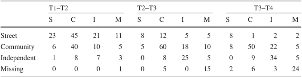
As an illustration of our methodology, data from the McKinney Homeless Research Project (MHRP) in San Diego as described in chapters 10 and 11 in the book by
Hedeker and Gibbons(2006), will be used. The aim of this project was to evaluate the effectiveness of using an incentive (a so-called Section 8 incentive) as a means of providing independent housing to homeless people with severe mental illness. A sample of 361 individuals took part in this longitudinal study and were randomly assigned to the experimental or control condition. Individuals’ housing status was assessed using three categories (living on the street (S)/living in a community center (C)/living independently (I)). As in many longitudinal data sets, some observations are missing at specific time points. We will use missing (M) as a fourth response category. Measurements are taken at baseline and at 6, 12, and 24 month follow up. Since we will be specifically interested in transitions the transition rates for the control condition
and the experimental condition are shown in Tables3and4respectively.
Ta b le 1 Relati v e bias in the p ersistent condition int I (
Y(−
1 ) = B ) I (
Y(−
1 ) = C ) GI (
Y(−
1 ) = B ) × GI (
Y(−
1 ) = C ) × G Dimension 1 ests − 0 . 05 1 . 12 0 . 53 0 . 21 − 0 . 43 − 0 . 16 mcar 0 . 00 − 0 . 00 0 . 01 0 . 00 − 0 . 01 − 0 . 02 mar1 0 . 00 − 0 . 01 0 . 00 0 . 01 − 0 . 00 − 0 . 00 mar2 0 . 00 − 0 . 01 − 0 . 02 − 0 . 01 0 . 00 0 . 02 mnar 0 . 00 − 0 . 01 0 . 01 0 . 00 − 0 . 01 − 0 . 00 Dimension 2 ests − 0 . 05 0 . 56 1 . 08 0 . 21 − 0 . 22 − 0 . 51 mcar − 0 . 00 − 0 . 00 0 . 01 0 . 00 − 0 . 02 − 0 . 02 mar1 0 . 00 − 0 . 01 − 0 . 01 − 0 . 00 0 . 01 0 . 01 mar2 0 . 00 − 0 . 00 − 0 . 03 − 0 . 00 − 0 . 01 0 . 02 mnar 0 . 07 − 0 . 00 − 0 . 01 − 0 . 00 − 0 . 02 0 . 01 The columns represent the v alues for the 12 parameters o f the model in E q. 8 . T he ro ws represent the four missingness conditions. T he line represented by ests pro v ides parameter estimates in a sample w ith size n = 10 , 000 ,r epresentati v e of a population. The column under “int” represents the intercept, I ( Y− 1 = B ) represents the ef fect when the p re vious response
Y(−
Ta b le 2 Relati v e bias in the h igh-change condition int I (
Y(−
1 ) = B ) I (
Y(−
1 ) = C ) GI (
Y(−
1 ) = B ) × GI (
Y(−
1 ) = C ) × G Dimension 1 ests 0 . 86 − 0 . 69 − 0 . 35 0 . 20 − 0 . 41 − 0 . 16 mcar 0 . 00 − 0 . 01 − 0 . 00 − 0 . 02 0 . 06 0 . 02 mar1 − 0 . 00 0 . 02 − 0 . 00 − 0 . 01 0 . 05 0 . 02 mar2 0 . 00 0 . 00 − 0 . 00 − 0 . 00 0 . 02 0 . 01 mnar 0 . 01 0 . 01 − 0 . 01 − 0 . 02 0 . 04 0 . 02 Dimension 2 ests 0 . 85 − 0 . 38 − 0 . 69 0 . 57 − 0 . 21 − 0 . 56 mcar − 0 . 00 − 0 . 00 0 . 00 − 0 . 02 0 . 02 0 . 03 mar1 0 . 00 0 . 01 0 . 01 − 0 . 01 − 0 . 00 0 . 02 mar2 − 0 . 00 − 0 . 01 0 . 01 0 . 00 − 0 . 00 0 . 00 mnar 0 . 07 0 . 00 0 . 01 − 0 . 02 0 . 01 0 . 02 The columns represent the v alues for the 12 parameters o f the model in E q. 8 . T he ro ws represent the four missingness conditions. T he line represented by ests pro v ides parameter estimates in a sample w ith size n = 10 , 000 ,r epresentati v e of a population. The column under “int” represents the intercept, I ( Y− 1 = B ) represents the ef fect when the p re vious response
Y(−
Table 3 Transition frequencies over time for the control group
T1–T2 T2–T3 T3–T4
S C I M S C I M S C I M
Street 23 45 21 11 8 12 5 5 8 1 2 2
Community 6 40 10 5 5 60 18 10 8 50 22 5
Independent 1 8 7 3 0 8 25 5 0 9 34 5
Missing 0 0 0 1 0 5 0 15 2 6 3 24
Table 4 Transition frequencies over time for the experimental group
T1–T2 T2–T3 T3–T4
S C I M S C I M S C I M
Street 11 28 37 4 9 0 4 2 11 5 2 1
Community 3 13 45 14 7 12 20 6 0 16 4 3
Independent 1 4 19 2 3 9 85 4 4 13 94 4
Missing 0 0 0 0 0 2 6 12 4 2 3 15
such zeros lead to parameter estimates that tend to plus or minus infinity. Using dimen-sion reduction in a distance framework these problems do not occur.
With these data we can pose ourselves the following questions:
1. Are the transitions homogeneous over time? 2. Are the transitions homogeneous over groups?
3. Are the transitions homogeneous over time and groups?
5.1 Models for MHRP data
We denote the predictor variables byPfor previous response,Gfor treatment group,
andT for time. The variableG is dichotomous with G = 0 for the control group
andG =1 for the experimental group. Following general log-linear notation, main
effects are denoted by single letters while interactions are denoted by adjacent letters,
i.e. P G denotes an interaction between previous response and treatment and P GT
indicate a three variable interaction. Only hierarchical models are used, meaning that if an interaction is present also the underlying main effects are present in the model. The research questions are translated in the following models of interest
M1 (P)Only the previous status has an influence on the current status. This influ-ence is the same for both the treatment group and the control group and is homogeneous over time;
M2 (P,G)Previous status plus treatment has influence on the current status, they
have an additive effect on the log odds;
M3a (P,G,Tl)Previous status plus treatment and time have an influence on current
M3b (P,G,Tc)Previous status plus treatment and time have an influence on current
status. Time is treated in a discrete way;
M4a (P G,Tl)The interaction between previous status and treatment plus a main
effect of time influence the current status. Time is treated in a linear way;
M4b (P G,Tc)The interaction between previous status and treatment plus a main
effect of time influence the current status. Time is treated in a discrete way;
M5a (G,P Tl)The interaction between previous status and time plus a main effect
of treatment influence the current status. Time is treated in a linear way;
M5b (G,P Tc)The interaction between previous status and time plus a main effect
of treatment influence the current status. Time is treated in a discrete way;
M6a (P G,P Tl)The interaction between previous status and time plus a an
interac-tion of previous status and treatment influence the current status. Time is treated in a linear way;
M6b (P G,P Tc)The interaction between previous status and time plus a an
interac-tion of previous status and treatment influence the current status. Time is treated in a discrete way;
M7a (P G,P Tl,GTl)The interaction between previous status and time, an
interac-tion of previous status and treatment influence the current status. Time is treated in a linear way;
M7b (P G,P Tc,GTc)The interaction between previous status and time plus a an
interaction of previous status and treatment influence the current status. Time is treated in a discrete way;
M8a (P GTl)The three-way interaction between previous status, time, and treatment
influence the current status. Time is treated in a linear way;
M8b (P GTc)The three-way interaction between previous status, time, and treatment
influence the current status. Time is treated in a discrete way.
5.2 Model selection
The AIC/QIC statistic for each of the described models is given in Table5, where it
can be seen that the model with all pairwise interactions and time used in a linear way has the smallest AIC. In fact, it is quite a bit lower than all other models except for Model 8a which is a more complex model. The model probability for Model 7a is
0.98, the evidence ratio compared to the second best model equals 0.98/0.02=49,
indicating that the support of model 7ais 49 times that of model 8a.
5.3 Model interpretation
The final selected model has the following linear predictor for the subjects positions
on dimensionm
ηi tm =αm+β1mI(Yi(−1)=C)+β2mI(Yi(−1)=I)+β3mI(Y(−1)=M)
+β4mGi+β5mTi t+β6mI(Yi(−1)=C)Gi
+β7mI(Yi(−1)=I)Gi+β8mI(Yi(−1)=M)Gi
+β9mI(Yi(−1)=C)Ti t+β10mI(Yi(−1)=I)Ti t+β11mI(Yi(−1)=M)Ti t
Table 5 AIC/QIC values and number of parameters (npar) for the models of interest
AIC/QIC npar Δk wk
M1 2374.60 11.00 130.60 0.00
M2 2309.46 13.00 65.46 0.00
M3a 2288.48 15.00 44.48 0.00
M3b 2313.63 17.00 69.64 0.00
M4a 2283.54 21.00 39.54 0.00
M4b 2286.14 23.00 42.15 0.00
M5a 2290.98 21.00 46.98 0.00
M5b 2274.45 29.00 30.45 0.00
M6a 2295.37 27.00 51.37 0.00
M6b 2272.67 35.00 28.67 0.00
M7a 2244.00 29.00 0.00 0.98
M7b 2259.36 39.00 15.36 0.00
M8a 2252.34 35.00 8.34 0.02
M8b 2275.21 51.00 31.22 0.00
C
I M
S
S0 S1
C0
C1
I0
I1 M0
M1
Fig. 1 Solution of the model with pairwise interactions between previous vote, treatment and time.SStreet,
0.1 0.2 0.3 0.4 0.5
−1.0 0.0 0.5 1.0 1.5 2.0
−0
.5
0.
00
.5
1.
01
.5
C I M S
Probabilities for Street
0.1
0.2
0.3
0.4
0.5
0.6
−1.0 0.0 0.5 1.0 1.5 2.0
−0.5
0.0
0.5
1.0
1.5
C I M S
Probabilities for Community House
0.1 0.2 0.3
0.4
0.5 0.6 0.7
0.8
0.9
−1.0 0.0 0.5 1.0 1.5 2.0
−0.5
0.0
0.5
1.0
1.5
C I M S
Probabilities for Independent
0.1 0.2
0.3 0.4
0.5 0.6
0.7
−1.0 0.0 0.5 1.0 1.5 2.0
−0.5
0.0
0.5
1.0
1.5
C I M S
Probabilities for Missing
Fig. 2 Contour lines of equal probabilities for each of the four categories of the response variable.SStreet,
Ccommunity house,Iindependent,Mmissing,1incentive group,0control group
where I(·)is the indicator function. The three terms I(Yi(−1) =C),I(Yi(−1)= I),
and I(Yi(−1) = M)jointly represent the variable P, previous state; The termGi
indicates whether a personi receives treatment (Gi = 1) or not (Gi = 0). The
variableTi trepresents time, with codes 0, 1, and 2. This is a complicated model, every
variable has an interaction with each other variable on the prediction of the response. The graphical solution of the model is given in Fig.1. In this graph the four classes of the responses are given together with prediction regions. The prediction regions specify areas where the probability for a certain category are highest. The decision boundaries are exactly at equal distances of two class points. In the upper region the class Missing is most probable, while at the left hand side the class Living on the Street is most probable. The probabilities for each category are visualized in Fig.2by a contour plot, giving lines of subjects’ positions with a constant probability for a given class. These can be used in combination with Fig.1to provide actual probabilities for all categories.
C
I M
S
S0 S1
C0
C1
I0
I1 M0
M1
Fig. 3 Individual trajectory of a subject receiving the incentive who lives on the street at T1, lives indepen-dently at T2, and lives on the street again at T3.SStreet,Ccommunity house,Iindependent,Mmissing,1
incentive group,0control group
That is, for a person that lived in a community house on the previous time point and did not obtain treatment (i.e. the C0 group), the arrow gives the positions atT = 0, 1, and 2 respectively where 0 is at the tail of the arrow, 2 is at the head andT =1 in the middle. The fact that the categories for Community house are moving shows that the Markov chain is not homogeneous. Of note is that these ‘groups’ are not formed by a constant group of individuals, i.e., for a subject in the control condition living on the street at the start but making a transition towards living in a community house, (s)he starts in group S0 and later on is in group C0.
It can be seen that subjects who receive the incentive and who live on the street at T1 (the arrow indicated by S1) have a high probability of a transition towards living inde-pendently (I) or towards living in a community center (C), i.e. this position is almost on the boundary between these two class points somewhat nearer to living indepen-dently. For the same category at T2, however, the probability for a transition towards living independently became smaller and the probability of a transition towards living in a community house is larger. Also, the probability of no transition, i.e. keep living on the street, became larger. For the same previous status at T3, the probability of a transition towards living independently strongly diminished, and chances are highest for no transition.
between T1 and T2 and between T2 and T3; from T3 to T4 the probability of staying on the street is the highest.
For subjects in the control condition and who live in a community house (The C0 group) the probability are rather high to stay in the community house. In contrast, subjects that receive the incentive and who live in a community house have a high probability to transit to living independently, but this probability becomes smaller over time.
For subjects that live independently and received the incentive (arrow indicated by I1) the probability is quite high (>0.8) to keep living independently; for those that live independently and did not receive the incentive (arrow indicated by I0) the probability of no transition is also highest and this probability becomes larger over time.
It should be noted that the arrows do not represent individual trajectories. Indi-vidual trajectories are characterized by the coordinatesηi t m. For every time point,
t = 1, . . . ,Ti, subjecti has a positionηi t in the Euclidean space. Joining the ηi1,
ηi2, andηi3gives an individual trajectory. For example, a subject who starts in the
treatment group and who is living on the street at T1 and makes a transition towards living independently makes a ‘jump’ from the S1 arrow towards the I1 arrow. When this person transits back between T2 and T3 (s)he ‘jumps’ towards the arrow head of the S1 arrow. This individual trajectory is indicated in Fig.3. At every time point the subject has a set of probabilities for the response variable, defined by the position of the subject and the distances towards each of the response category points.
5.4 Previous MHRP analyses
Hedeker and Gibbons(2006) analyzed the data using a mixed effect multinomial logit
model andDe Rooij and Schouteden(2012) provide a graphical representation of that
model. The mixed effect multinomial logit model looks at the temporal development of the three category probabilities for the two groups. The results presented inHedeker and Gibbons(2006) andDe Rooij and Schouteden(2012) suggest that the subjects in the treatment group have higher probability to be in the Independent Living condition, although this probability declines at the end of the study. For the control condition the probability of Living on the Street also becomes smaller. The same conclusions can be derived from our model. For the treatment group, all arrows start in the region for Independent living or close to that (M1). The head of these arrows are closer to other regions indicating that the probabilities to transit towards either a Community house or Living on the Street become larger.
6 Discussion
Such a transitional approach was developed within a distance framework. The distance framework has several advantages compared to a multinomial regression model. First, dimension reduction is possible such that the number of parameters is kept low compared to the multinomial regression model. Furthermore, the distance approach is not as vulnerable to empty cells as the multinomial regression model. Therefore, in cases where parameter estimates of the multinomial regression model do not exist, the IPC model may still be estimable.
In longitudinal data often missing values occur. Within the modeling framework we created one extra category in the response variable. As such, we created a model for the simultaneous analysis of the response and the missingness. Treating missing values as an extra category of the response variable seems a promising way to deal with missing values. It hardly complicates the analysis and, although the Monte Carlo study was limited, the results are promising.
In our Monte Carlo study we investigated a three category multinomial regression model. When missing data occur, a four category multinomial model is obtained. No dimension reduction was utilized in the Monte Carlo study. It should be noted that for binary outcome variables, that are much more common than multinomial ones, with missing values a multinomial model with three categories is obtained that can be fitted using the IPC model in two dimension. That is, having longitudinal binary data with missing values an IPC model may be utilized in two dimensions to obtain unbiased parameter estimates. Moreover, using this approach we also obtain insight in the relationship between explanatory variables and drop out.
In our Monte Carlo study we found that the results obtained with missing data are almost the same as obtained on complete data, even in the Missing Not at Random situation. Although this seems promising, care should be taken, because the mecha-nism by which the missing values are treated and why this results in almost unbiased results is not completely understood. At least in the MNAR condition more bias was expected. Further simulation studies and theoretical work is needed in order to com-pletely understand the process. A line of reasoning about the process is as follows. For MNAR situations a model that jointly models the responses and the missingness
is often needed. Two types of models are distinguished by Molenberghs and
Ver-beke(2005): selection models and pattern mixture models.Albert(2000) discusses a transitional model for longitudinal binary data where missingness may occur. He dis-tinguishes between intermittent missingness and drop-out and developed a transition model that deals with non-ignorable missingness, i.e. missing values that do depend on the otherwise observed value. Therefore, he developed a joint model where the
responses follow ak-th order Markov model and the missingness follows a first order
Markov model, where missingness is dependent on the current (possibly missing) response. An EM algorithm was proposed for fitting the model. In our case we also jointly model the responses and missingness, but in a rather simple way: we just added an extra category to our response variable. It should be noted that this changes the def-inition and interpretation of the model. However, it is well known that a multinomial regression can be fitted using separate binary logistic regressions (Agresti 2002).
probabilities change over time. The selected model incorporates three interaction terms which makes a traditional multinomial logit model very difficult to interpret. Our graphical representation in Fig.1helps to get a clearer interpretation. In the application dimension reduction was applied, while in the Monte Carlo study models were fitted in the highest dimensionality. How parameters are recovered using the proposed method for missing data when also dimension reduction is applied is unknown. Therefore, more extensive simulation studies are needed. This issue could affect the results in our application.
All models and analyses were performed in R. R-code of both the Monte Carlo study as well as the empirical data analysis can be obtained from the website of the
author,http://www.markderooij.info.
Open Access This article is distributed under the terms of the Creative Commons Attribution 4.0 Interna-tional License (http://creativecommons.org/licenses/by/4.0/), which permits unrestricted use, distribution, and reproduction in any medium, provided you give appropriate credit to the original author(s) and the source, provide a link to the Creative Commons license, and indicate if changes were made.
References
Agresti A (2002) Categorical data analysis. Wiley, New York
Akaike H (1973) Information Theory as an extension of the maximum likelihood principle. In: Petrov BN, Csake F (eds) Second international symposium of information theory. Akademia Kiado, Budapest, pp 267–281
Albert PS (2000) A transitional model for longitudinal binary data subject to nonignorable missing data. Biometrics 56:602–608
Anderson DR (2008) Model based inference in the life sciences. Springer, New York
Bartolucci F, Farcomeni A, Pennoni F (2013) Latent Markov models for longitudinal data. Chapman and Hall/CRC, Boca Raton
Bonney GE (1987) Logistic regression for dependent binary observations. Biometrics 43:951–973 Cheng G, Yu Z, Huang JZ (2013) The cluster bootstrap consistency in generalized estimating equations. J
Multivar Anal 115:33–47
De Rooij M (2009a) Ideal point discriminant analysis revisited with a special emphasis on visualization. Psychometrika 74:317–330
De Rooij M (2009b) Trend vector models for the analysis of change in continuous time for multiple groups. Comput Stat Data Anal 53:3209–3216
De Rooij M (2011) Transitional ideal point models for longitudinal multinomial outcomes. Stat Model 11:115–135
De Rooij M (2012) An application of the mixed effects trend vector model to asymmetric change data with auxiliary variables. Behaviormetrika 39:75–90
De Rooij M, Schouteden M (2012) The mixed effects trend vector model. Multivar Behav Res 47:635–664 De Rooij M, Worku HM (2012) A warning concerning the estimation of multinomial logistic models with
correlated responses in SAS. Comput Methods Programs Biomed 107:341–346
Diggle PJ, Heagerty P, Liang K-Y, Zeger SL (2002) Analysis of longitudinal data. Oxford University Press, Oxford
Donders ART, Van der Heijden GJMG, Stijnen T, Moons KGM (2006) Review: a gentle introduction to imputation of missing values. J Clin Epidemiol 59:1087–1091
Eliason SR (1993) Maximum likelihood estimation: theory and logic. Sage Publications, Newbury Park Enders CG (2010) Applied missing data analysis. The Guilford Press, York
Fox J, Anderson R (2006) Effect displays for multinomial and proportional odds logit models. Sociol Methodol 36:225–255
Hedeker D, Gibbons RD (2006) Longitudinal Data Analysis. Wiley, Hoboken
Jeliˇci´c H, Phelps E, Lerner RM (2009) Use of missing data methods in longitudinal studies: the persistence of bad practices in developmental psychology. Dev Psychol 45:1195–1199
Liang K-Y, Zeger SL (1986) Longitudinal data analysis using generalized linear models. Biometrika 73:13– 22
Little RJ, Rubin DB (2002) Statistical analysis with missing data. Wiley, New York Meulman J (1982) Homogeneity analysis of incomplete data. DSWO Press, Leiden Molenbergs G, Verbeke G (2005) Models for discrete longitudinal data. Springer, Berlin
Paik MC (1988) Repeated measurement analysis for nonnormal data in small samples. Commun Stat Simul Comput 17:1155–1171
Pan W (2001) Akaike’s information criterion in generalized estimating equations. Biometrics 57:120–125 Rubin DB (1976) Inference and missing data. Biometrika 63:581–592
Sherman M, Le Cessie S (1997) A comparison between bootstrap methods and generalized estimating equations for correlated outcomes in generalized linear models. Commun Stat Simul Comput 26:901– 925