RURAL LIVELIHOODS AND ENVIRONMENTAL CHANGE IN UGANDA
Maia Averyl Call
A dissertation submitted to the faculty at the University of North Carolina at Chapel Hill in partial fulfillment of the requirements for the degree of Doctor of Philosophy in the Department
of Geography in the College of Arts and Sciences.
Chapel Hill 2017
ABSTRACT
Maia Averyl Call: Rural Livelihoods and Environmental Change in Uganda (Under the direction of Clark Gray)
Environmental changes, which include soil degradation, deforestation, and climate change, have long been posited as potential drivers of rural livelihood decisions in Sub-Saharan Africa. However, providing empirical evidence for these socio-environmental patterns has proven difficult due to a lack of spatially explicit longitudinal livelihoods data as well as appropriately fine-scale environmental data. To address this gap in the literature, this dissertation spatially links two waves of longitudinal household and plot survey data (collected in Uganda in 2003 and 2013) with a remotely sensed forest cover product and modeled climate data. These data provide a unique opportunity to quantitatively address three questions central to the topic of
ACKNOWLEDGEMENTS
When I was finishing up my Geography undergraduate degree at UNC-Chapel Hill back in 2012 and struggling to make a decision about where to go for graduate school, one of the professors in the department offered me a piece of advice. He said that no matter where I chose to go for graduate school, I would look back one year from then and feel like I had made the right choice. He was not wrong. Looking back at my five years of graduate school in the UNC-Chapel Hill Geography department, as well as my four previous years of undergraduate work, I can only say that I feel incredibly privileged to have had the opportunity to learn from and work with so many brilliant and dedicated scholars and teachers.
I first wish to thank my outstanding advisor, Clark Gray. Over the course of the five years of this program, he has continuously been there to rapidly respond to my (sometimes panicked) emails, talk me through the dark moments I have lost faith in the analysis for a paper, and help me develop creative solutions to difficult problems. He has also provided me with a wealth of institutional knowledge and guidance along the esoteric path toward becoming an academic.
things. Finally, the soils course I took at Duke with Dan Richter first got me excited about soil and gave me the toolkit necessary to understand soil fertility, as well as introducing me to one of my favorite books of all time: Dirt: The ecstatic skin of the earth. I also wish to acknowledge funding support from the Carolina Population Center as well as the UNC Graduate School.
The doctoral process is of course about conducting research, but it is also about learning how to be an academic, and teaching is an important element of academic life. In this vein, I want to particularly thank Ashley Ward and Gabriela Valdivia, both of whom have been invaluable in teaching me how to teach. Through their mentorship, I now feel comfortable designing a course, working with undergraduates, and thinking through a range of approaches to effective instruction.
TABLE OF CONTENTS
CHAPTER 1: INTRODUCTION ... 1
Introduction ... 1
References ... 5
CHAPTER 2: RECONCILING THE DEBATE: PERCEIVING AND MEASURING SOIL FERTILITY IN UGANDA ... 7
Introduction ... 7
Background ... 9
Methods ... 13
Results and Discussion ... 19
References ... 24
Tables ... 28
CHAPTER 3: WHAT DRIVES ENVIRONMENTAL MIGRANTS? LONGITUDINAL EVIDENCE FROM UGANDA ... 33
Introduction ... 33
Background ... 35
Data Collection ... 38
Analysis ... 41
Results and Discussion ... 45
Conclusions ... 50
References ... 53
Tables ... 58
CHAPTER 4: CLIMATE ANOMALIES AND SMALLHOLDER LIVELIHOODS IN UGANDA ... 64
Introduction ... 64
Background ... 65
Methods ... 69
Results and Discussion ... 77
Conclusions ... 79
References ... 82
Tables ... 88
CHAPTER 5: CONCLUSIONS ... 94
Conclusions ... 94
References ... 98
APPENDIX B: GPS DATA... 102
APPENDIX C: ATTRITION ... 103
APPENDIX D: SPATIAL MATCHING ... 105
APPENDIX E: FULL AND RESTRICTED SAMPLE... 107
CHAPTER 1: INTRODUCTION
Introduction
Environmental changes have long been posited as drivers of rural livelihood decisions. In Sub-Saharan Africa, these environmental changes have been largely viewed in a negative light. For the past century, researchers have argued that soil fertility is degrading in the region, driven by rapid population growth (Stocking, 2003; Stoorvogel & Smalling, 2000; Wortmann & Kaizzi, 1998). Fears that population growth is also driving deforestation in the region have also emerged in recent decades (Geist & Lambin, 2002; Rudel, 2013). Sub-Saharan Africa is also considered by the Intergovernmental Panel on Climate Change to be a near term hot spot for the negative ramifications of climate change, with temperatures expected to rise and rainfall predicted to become more spatially and temporally unpredictable (IPCC, 2014). Taking into consideration that Sub-Saharan Africa is a region with high rates of poverty (Barrett, 2008), high population growth rates (Caldwell & Caldwell, 1990), a heavy reliance on natural resource based
livelihoods (e.g. agriculture) (Ellis, 2000), and lack of market access due to market failures as well as poor infrastructure (Dorosh, Wang, You, & Schmidt, 2012; Linard, Gilbert, Snow, Noor, & Tatem, 2012), researchers have predicted that environmental changes may drive large-scale crop failure (Kotir, 2011), forced migration (Warner, 2010), and pressure to divest from agricultural livelihoods (Loison, 2015).
influences on livelihoods. In this dissertation, I draw together two waves of longitudinal household and plot survey data collected in Uganda in 2003 and 2013 with a remotely sensed forest cover product (Hansen et al., 2013) and gridded climate data (Hijmans, Cameron, Parra, Jones, & Jarvis, 2005; UEACRU et al., 2013) via a spatial linkage. These data allow me to quantitatively address three questions central to the broad subject of environmental change and rural livelihoods: 1) What is the relationship between perceived and measured soil fertility and soil degradation?; 2) How do environmental factors inform temporary and permanent migration decisions?; and 3) How do climate anomalies shape on-farm and off-farm smallholder livelihood strategies?
I address the first question in chapter two, where I explore the relationship between perceived and measured soil fertility and soil degradation. As a primary contributor to agricultural productivity, soil fertility is an essential part of rural livelihoods in Sub-Saharan Africa. Concerns about soil degradation in the region have been fueled in recent years by rapid population growth. While scholars have attempted to assess soil fertility in the region for decades, differences in methodologies, study sites, and theoretical approaches have resulted in heterogeneous and divergent findings. One of the major debates arising out of this work focuses on the value and veracity of farmers’ perceptions and laboratory measures of soil fertility and soil degradation. Some scholars have argued that one more accurately reflects true soil fertility/degradation, while others have concluded that they are interchangeable. These
analysis employs multilevel modeling techniques and draws upon a large-sample
socio-environmental household survey collected in Uganda in 2003 and 2013. This approach reveals that soil fertility perceptions and measures are complementary but that farmers’ perceptions of soil degradation appear to be based on landscape scale observations rather than chemical properties. Together, perceived and measured soil fertility are strong independent predictors of crop productivity, suggesting that laboratory measures may not be picking up all of the elements of soil fertility. Farmers’ perceptions thus have the potential to provide valuable information on soil fertility, in combination with laboratory measures.
In the fourth and final substantive chapter, I investigate the relationship between climate anomalies and smallholder livelihood strategies. Sub-Saharan Africa is one of the regions of the world considered most critical in terms of the negative effects of global climate change. On-farm agricultural strategies and off-farm livelihood diversification into non-natural resource based livelihoods are the two major ways in which people are theoretically expected to respond to climate anomalies. However, few studies have examined the empirical implications of climate anomalies on these in situ adaptation strategies. Responding to this gap in the literature, we use regression approaches to analyze two waves of household survey data, spatially linked with climate data for rural Uganda. We find that household livelihoods are responsive to climate over short and long time scales. Droughts decrease agricultural productivity in the short term only, reducing individual livelihood diversification in the long term. Higher temperatures can be coped with in the short term, but in the long run above average temperatures lower agricultural
REFERENCES
Barrett, C. B. (2008). Poverty Traps and Resource Dynamics in Smallholder Agrarian Systems.
Applied Economics, 31(1973), 17–40. Retrieved from http://www.springerlink.com/index/l781l33u3u14m50l.pdf
Caldwell, J. C., & Caldwell, P. (1990). High Fertility In Sub-Saharan Africa. Scientific American, (May), 118–125.
Dorosh, P., Wang, H. G., You, L., & Schmidt, E. (2012). Road connectivity, population, and crop production in Sub-Saharan Africa. Agricultural Economics, 43(1), 89–103.
https://doi.org/10.1111/j.1574-0862.2011.00567.x
Ellis, F. (2000). Rural livelihoods and diversity in developing countries. Oxford university press. Geist, H. J., & Lambin, E. F. (2002). Proximate Causes and Underlying Driving Forces of
Tropical Deforestation. BioScience, 52(2), 143. https://doi.org/10.1641/0006-3568(2002)052[0143:PCAUDF]2.0.CO;2
Hansen, M. C., Potapov, P. V, Moore, R., Hancher, M., Turubanova, S. a, Tyukavina, a, … Townshend, J. R. G. (2013). High-resolution global maps of 21st-century forest cover change. Science (New York, N.Y.), 342(6160), 850–3.
https://doi.org/10.1126/science.1244693
Hijmans, R. J., Cameron, S. E., Parra, J. L., Jones, P. G., & Jarvis, A. (2005). Very high resolution interpolated climate surfaces for global land areas. International Journal of Climatology, 25(15), 1965–1978. https://doi.org/10.1002/joc.1276
IPCC. (2014). Summary for policymakers. In and L. L. W. Field, C.B., V.R. Barros, D.J. Dokken, K.J. Mach, M.D. Mastrandrea, T.E. Bilir, M. Chatterjee, K.L. Ebi, Y.O. Estrada, R.C. Genova, B. Girma, E.S. Kissel, A.N. Levy, S. MacCracken, P.R. Mastrandrea (Ed.),
Climate Change 2014: Impacts, Adaptation, and Vulnerability. Part A: Global and Sectoral Aspects. Contribution of Working Group II to the Fifth Assessment Report of the
Intergovernmental Panel on Climate Change (pp. 1–32). Cambridge, United Kingdom and New York, NY, USA: Cambridge University Press.
Kotir, J. H. (2011). Climate change and variability in Sub-Saharan Africa: A review of current and future trends and impacts on agriculture and food security. Environment, Development and Sustainability, 13(3), 587–605. https://doi.org/10.1007/s10668-010-9278-0
Linard, C., Gilbert, M., Snow, R. W., Noor, A. M., & Tatem, A. J. (2012). Population
distribution, settlement patterns and accessibility across Africa in 2010. PLoS ONE, 7(2). https://doi.org/10.1371/journal.pone.0031743
Loison, S. A. (2015). Rural Livelihood Diversification in Sub-Saharan Africa : A Literature Review. The Journal of Development Studies, 51(9), 1125–1138.
Philosophical Transactions of the Royal Society of London. Series B, Biological Sciences,
368(1625), 20120405. https://doi.org/10.1098/rstb.2012.0405
Stocking, M. a. (2003). Tropical soils and food security: the next 50 years. Science, 302, 1356– 1359. https://doi.org/10.1126/science.1088579
Stoorvogel, J. J., & Smalling, E. M. A. (2000). Assessment of soil nutrient depletion in Sub-Saharan Africa: 1983-2000. Soil and Water (Vol. II). Wageningen.
CHAPTER 2: RECONCILING THE DEBATE: PERCEIVING AND MEASURING SOIL FERTILITY IN UGANDA
Introduction
Soil fertility, the ability to provide crops with the essential nutrients to promote growth, is an integral element of rural livelihoods in rural Sub-Saharan Africa. For decades, scholars have attempted to accurately assess soil fertility in the region (Palm, Sanchez, Ahamed, & Awiti, 2007). These efforts were originally borne out of a social and historical context that fostered the concern that population growth and poverty were driving soil degradation, a process that
includes erosion and nutrient depletion (Palm et al., 2007). In recent years, unprecedented population growth, stagnating crop yields, and concerns about global climate change have led to a resurgence of this narrative (Muchena, Onduru, Gachini, & de Jager, 2005; Sanchez, 2002; Tully, Sullivan, Weil, & Sanchez, 2015). Despite over a century of research on soil fertility and degradation in the region, variations in methodological approaches, study sites, and
Embedded within this interdisciplinary debate is a matter of practical concern. Farmers and agronomists may be coming to their, perhaps differing, conceptions of soil fertility and soil degradation based on very different perspectives and information. Much previous research has suggested that farmers’ perceptions are based on factors such as crop yield and the number and kinds of weeds present in the field (E. Barrios et al., 2006; Gruver & Weil, 2007; Murage, Karanja, Smithson, & Woomer, 2000). Perceptions also have the potential to be shaped by external sociocultural elements, such as distance to the nearest marketplace or the relative wealth of neighbors (Briggs, 2013; Corbeels, Shiferaw, & Haile, 2000; Desbiez, Matthews, Tripathi, & Ellis-Jones, 2004; Ericksen & Ardón, 2003; Maconachie, 2012; Marenya, Barrett, & Gulick, 2008; Sillitoe, 1998). Agronomists, on the other hand, rely mostly upon biochemical
measurements, such as carbon content, pH, and soil texture, to assess soil fertility and
degradation. Policies implemented, or soil improvement measures suggested, based on measured soil fertility may have low uptake by farmers if farmers do not likewise perceive a problem with their soil fertility.
conversely, appear to be based on erosion and landscape scale observations and are not associated with chemical laboratory measures. Together, both perceived and measured soil fertility are strong predictors of plot productivity. This finding suggests that biophysical measures may not be picking up all of the elements of soil fertility that contribute to crop
production. Farmers’ perceptions can contribute valuable information to the determination of soil fertility, in combination with laboratory measures.
Background
Over the past three decades, scholars across a range of disciplines have turned their attention to the relationship between scientific and local knowledge. Findings from these studies have demonstrated that a singular, broadly applicable and transferable approach may not always provide the best results if applied without the recognition of cultural variability and socio-environmental complexity. Ethnopedology, “a hybrid discipline nurtured by natural as well as social sciences [that] encompasses the soil and land knowledge systems of rural populations, from the most traditional to the most modern” (Barrera-Bassols & Zinck, 2003), emerged during this multidisciplinary turn.
perceptions of soil fertility are one factor that drives agricultural management decisions (E. Barrios et al., 2006; Gruver & Weil, 2007; Murage et al., 2000). In recent years, however, scholars have argued that it is not enough to compare and categorize soil fertility measures in a vacuum (Briggs, 2013). Responding to these concerns, a number of researchers over the past several decades have examined how farmers’ perceptions and laboratory measures of soil fertility relate to one another within their socio-environmental context (Berazneva, Mcbride, Sheahan, & David, 2016; Dawoe, Quashie-Sam, Isaac, & Oppong, 2012; Desbiez et al., 2004; L. C. Gray & Morant, 2003; Maconachie, 2012; Marenya et al., 2008; Odendo, Obare, & Salasya, 2010; Osbahr & Allan, 2003).
Studies that explore perceived and measured soil fertility have come to a wide range of differing conclusions. On one end of the spectrum, studies have found strong agreements between laboratory measures and farmers’ perceptions in Ghana (Dawoe et al., 2012), Kenya (Mairura et al., 2007; Murage et al., 2000), and northern Ethiopia (Corbeels et al., 2000).
More specifically, Dawoe and colleagues (2012) find that in the Ashanti region of Ghana, farmers’ indicators of soil fertility (or infertility) corresponds well with scientific assessment, and are unrelated to age, location, or gender of the head of household. Likewise, Desbiez and colleagues (2004) observe a strong relationship between scientific measures and perceptions of soil fertility in Nepal, but also argue that socio-environmental context, along with plot-specific characteristics, are an important element of how farmers assess fertility. Osbahr and Allan (2003), conversely, report no direct link between perceptions and scientific soil assessment in Niger. However, they argue that this is a result of the complex ethnopedological framework developed by farmers, which draws from social and cultural, as well as physical, environmental elements. Similarly, Maconachie (2012) concludes that the reason for the mismatch between farmers’ perceptions and laboratory measures outside Kano, Nigeria is that socio-environmental context—exposure to urban culture and consumerism—can skew farmers’ perceptions of their own soil productivity. Gray and Morant (2003) find that local and scientific measures of soil fertility change in southwestern Burkina Faso match poorly, perhaps because farmers’
perceptions of soil fertility are based on the social and economic changes in the region, rather than biophysical shifts.
Odendo and colleagues (2010) employ clustered, randomized sampling to gather perceptions data (N=331) representative of two different agro-ecological zones, one of which had higher agricultural potential than the other. No laboratory soil measures were gathered for
comparison—rather, Odendo and colleagues conclude that farmers’ perceptions were probably fairly accurate because their ways of measuring soil fertility (e.g. crop performance, crop color) were in accord with those used by agronomists in the field. These researchers then use
econometric methods to explore how well various socio-ecological contextual factors are able to predict perceptions of degradation. Odendo and colleagues find that agro-ecological zone, food self-sufficiency, and awareness of soil fertility management practices all had a significant relationship with perceptions of soil degradation.
provides policy-relevant insights into the relationship between farmers’ perceptions and laboratory measures of soil fertility.
Methods
Study location
Uganda is a rural country, with 87% of the nearly 35 million Ugandans living outside of urban areas (Uganda Bureau of Statistics, 2014). For the most part, the soils of Uganda are highly weathered Oxisols and Ultisols with low nutrient reserves for farmers to draw upon (Palm et al., 2007; Ssali & Vlek, 2002). The population of the country is growing at a rapid rate of 3.03% annually, and much of this population growth is in rural areas. Rural population density, already high in some regions, is predicted to increase with population growth (United Nations Development Programme, 2014). Many rural households depend on income from smallholder agriculture as their primary livelihood strategy, but within Uganda there is much heterogeneity in agro-ecological conditions, cultural context, land tenure regimes, and access to markets (Yamano & Kijima, 2010).
Data
The analysis utilizes plot-level panel data collected in rural Uganda. The first wave of these data was collected in 2003 by the International Food Policy and Research Institute (IFPRI) in collaboration with the National Agricultural Research Laboratories (NARL) of Uganda. Households selected for this survey were chosen from within a sampling framework developed by the Uganda Bureau of Statistics (UBOS) for a larger survey (Nkonya et al., 2008). Using clustered random sampling, households were selected from eight different UBOS survey districts in an effort to represent Uganda’s agro-ecological diversity (see Appendix F). In 2013,
Cornell University, Purdue University, and Brown University collaborated to carry out the second wave of this survey. In both waves, enumerators collected survey and spatial data at the household, plot, and community levels, and took plot-level soil samples for laboratory soil analysis (see Appendix 1 for soil sampling and analysis procedures; see Appendix 2 for spatial data procedures).
In the 2013 follow-up, enumerators were able to return to 727 of the 849 households successfully interviewed in 2003. Of the 122 households not successfully re-interviewed, all but 11 were not re-interviewed due to budgetary restrictions, rather than refusal to answer (see Appendix 3 for differences in tracked and lost households). In addition to the original
households, individuals who had split off to form new households in the intervening years were tracked and interviewed if they were still within the original parish. Including these split
households, enumerators collected data from 831 households in 2013. Soil samples were successfully collected and analyzed from 1,965 plots in 2003 and 1,389 plots in 2013 (full sample). Of these plots, a subsample of 715 can be successfully spatially matched across the two years (restricted sample) (see Appendix 4 for matching procedure; see Appendix 5 for
module on current crops cultivated and perceptions of plot level characteristics (including soil fertility and degradation).
Alongside these survey data, environmental data on precipitation and slope are drawn from two remotely sensed data sources. Average annual precipitation values for a given
community were extracted from the WorldClim Global Climate Dataset at a 1 kilometer spatial resolution using a 1 kilometer buffer around the community centroid (Hijmans et al., 2005). This buffer size was chosen based on the spatial distribution of agricultural plots from the survey. Slope was calculated using the ASTER Global Digital Elevation Map (DEM), which has a spatial resolution of 30 meters (LP DAAC, 2016).
have decreased over this time period. Without amendments, most phosphorus is found in the underlying bedrock and farmers may be decreasing phosphorus content in soil through continuous cropping. Plot productivity, which is measured as monetary value produced per hectare due to the variability in crop types present on each plot, appears to have increased threefold between 2003 and 2013.
Analysis
The analysis draws upon both the full and the restricted plot-level samples for 2003 and 2013. The full sample is used to analyze the extent to which laboratory measures predict farmers’ perceptions of soil fertility, as well as to explore the extent to which farmers’ perceptions and laboratory measures predict plot productivity. For these analyses, the two waves of data are stacked to increase sample size, controlling for the year of survey data collection. The restricted sample is employed to examine the extent to which change in laboratory measures can predict farmers’ perceptions of soil quality change between 2003 and 2013. For this model, the analysis is cross-sectional, with all variables originating from the 2013 survey other than the laboratory measures from 2003, which are included to control for survey baseline chemical properties.
collection. Because of these fixed effects, results can be interpreted s comparing plots in the same district in the same year. Values from the ordinal logistic regressions are shown as odds ratios. In all regressions, household asset values and household livelihoods value are transformed for normality, as they are highly right-skewed. Soil pH is included in the models as both a linear and squared term, as optimal pH for soil fertility is in the middle ranges of the scale.
Alongside perceived and measured soil fertility, a standard set of socio-demographic and environmental controls are employed in all models. Household level controls include the age, gender, and education level of the head of household, who is typically the person answering the survey questions. Differences in age, gender, and education have been shown to impact a farmer’s ability to assess the fertility of his soil (or to increase plot productivity), perhaps due to differences in experience and access to agronomic information. Likewise, participation in agricultural training is adjusted for in the models (Marenya et al., 2008). Previous research has suggested that household size can influence perceptions of soil fertility, regardless of actual soil fertility or productivity, because a larger household would require greater productivity to
when flooding and muddy conditions are common) are included. Market access has previously been seen to impact farmers’ perceptions by providing them with the opportunity to compare their soil fertility or living condition with those of a wider range of individuals (Maconachie, 2012). Further, access to markets and all-weather roads could improve the ability of households to obtain soil amendments or attend training courses at local farmers’ organizations.
Results and Discussion
Perceived and measured soil fertility and soil degradation
As one might expect from the complex and contradictory evidence found in the literature, it appears from the findings that the relationship between perceived and measured soil fertility and soil degradation is complicated. Examining the joint tests for soil fertility (Table 2), findings suggest that laboratory measures of soil fertility predict perceived soil fertility in both 2003 and 2013. However, in 2003 higher soil organic matter is associated with greater odds of perceived high soil fertility, while in 2013 only higher phosphorus is associated with higher soil fertility. Considering both years together through the stacked model, it appears that, as in 2003 alone, higher organic matter is significantly associated with higher odds of perceived higher soil fertility.
In addition to the positive and significant relationship between perceived and measured soil fertility, the findings suggest that that several household and plot characteristics are
significant predictors of perceived soil fertility. Though the joint test indicates that the overall relationship is not significant, in the stacked model, households that have received agricultural training have about one and a half times greater odds of perceiving their soil as more fertile. As many factors that may contribute to soil fertility, such as weed growth, management strategies, and labor time invested, are not observable through the laboratory measures, the significant and positive relationship between agricultural training and perceived soil fertility may be
representative of actual management strategies being employed to shape soil fertility. Through the joint test, it is clear that, in addition to the laboratory measures, several other plot
perceptions of soil fertility are encapsulating more about actual soil fertility than the chemical laboratory measures alone, which do not account for additional biophysical properties like topsoil depth and erosion.
In contrast, the cross-sectional analyses find no relationship at all between perceived and measured soil degradation (Table 3). Although the models include a number of covariates that have been shown in the literature to be related to perceived soil degradation in our model, few of them appear to be significant. Farmers appear to be generating their perceptions of soil
degradation through plot level characteristics, in particular topsoil depth and rill erosion. Plots with shallow topsoil and greater rill erosion are perceived as significantly degraded. From these findings, it is possible to conclude that the chemical properties tested by laboratory measures are difficult for farmers to observe changing over time, unlike easily observable processes like erosion. Farmers’ perceptions of soil degradation are therefore reflective of important landscape scale elements of soil degradation not accounted for by laboratory measures but not indicative of changes that may be occurring in the chemical properties of the soil.
Plot productivity, predicted by perceptions and laboratory measures
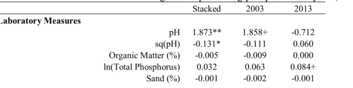
Both perceptions and laboratory measures are found to be positively associated with higher crop productivity per hectare (Table 4). In particular, more optimal pH is associated with higher productivity. As both perceived and measured soil fertility are significant in the same model, it is clear that perceptions and laboratory measures are complementary rather than substitutes for one another, each providing something different to the measurement of soil fertility.
male head of household with access to agricultural training and higher livestock and asset values is associated with higher crop productivity per hectare. Most of these characteristics are
reflective of an overall increased socio-economic status, which improves access to labor, improved seeds, and other factors that increase plot productivity. Increased distance to a local market is associated with decreased crop productivity per hectare, perhaps because increased distance makes it costlier to transport crops to market. Lack of access to markets may also de-incentivize farmers to produce a surplus for the purpose of sale.
Plots further away from a household appear to be more productive per hectare, as are those with greater topsoil depth. Greater topsoil depth is better for agriculture. Plots further from the household may be more recently cleared or fallowed, increasing their crop productivity when cultivated. Counterintuitively, sheet erosion is associated with to improved productivity. High productivity from intensive farming may, however, be the reason for the sheet erosion, as these questions were asked at the same points in time. Larger plots appear to be less productive per hectare than smaller plots, and increased slope is associated with decreased plot productivity. The inverse plot size-plot productivity relationship has been observed in a number of past studies, though the exact mechanisms for this relationship remain unclear (Bevis & Barrett, 2016). Crop productivity per hectare on all of the plots has increased between 2003 and 2013, likely due to more intensive management.
Conclusions
measures for fertility but not degradation. While it is possible that farmers’ perceptions of degradation might be inaccurate, it is equally possible that perceptions of degradation may just be capturing some additional element of soil degradation not expressed through laboratory measures of fertility change, such as erosion or weed growth. The results of the productivity analysis suggest that perceptions of fertility may be picking up something that laboratory assessments are not. Throughout the analysis, it is clear that context matters—socio-environmental characteristics contribute to farmers’ perceptions of soil fertility.
From a practical standpoint, these findings have several implications. It is very apparent from the results that there is a difference between the way that soil degradation is understood by laboratory measures and farmers’ perceptions. Perceived and measured soil fertility, on the other hand, can be seen as complementary. Many previous studies comparing perceptions and
measures have conflated soil fertility and soil degradation, and our observations demonstrate that this is highly problematic. Additionally, this analysis highlights the value of considering
perceptions alongside laboratory measures when trying to accurately assess multidimensional soil fertility for policy or research purposes (Agrawal, 1995).
The methodological significance of this analysis is threefold. First, the findings
demonstrate the utility of large-sample, clustered, randomly sampled plot-level longitudinal data for the investigation of questions surrounding soil degradation. Without longitudinal plot-level data, it is not possible to assess the processes of degradation. Second, these results reinforce the findings of previous researchers who have argued for the necessity of laboratory soil analysis, rather than simply relying on perceptions of soil fertility and degradation. While perceptions do appear to be related to laboratory measures of soil fertility, this is not the case in regard to degradation. It is clear from the analysis that perceptions are much more contextualized than laboratory measures, and are best used as complementary to, rather than as a substitute for, laboratory measures. Finally, the significance of context observed in this analysis argues for the importance of analyzing soil fertility within its socio-ecological context (Dawoe et al., 2012).
REFERENCES
Agrawal, A. (1995). Dismantling the divide between indigenous and scientific knowledge.
Development and Change, 26(3), 413–439. https://doi.org/10.1017/CBO9781107415324.004
Aynekulu, E., Carletto, C., Gourlay, S., & Shepherd, K. (2016). Collecting the Dirt on Soils: Advancements in Plot-Level Soil Testing and Implications for Agricultural Statistics. Barrera-Bassols, N., & Zinck, J. A. a. (2003). Ethnopedology: a worldwide view on the soil
knowledge of local people. Geoderma, 111(3–4), 171–195. https://doi.org/10.1016/S0016-7061(02)00263-X
Barrett, C. B. (1996). On price risk and the inverse farm size-productivity relationship. Journal of Development Economics, 51(2), 193–215.
https://doi.org/http://dx.doi.org/10.1016/S0304-3878(96)00412-9
Barrios, E., Delve, R. J., Bekunda, M., Mowo, J., Agunda, J., Ramisch, J., … Thomas, R. J. (2006). Indicators of soil quality: A South-South development of a methodological guide for linking local and technical knowledge. Geoderma, 135, 248–259.
https://doi.org/10.1016/j.geoderma.2005.12.007
Berazneva, J., Mcbride, L., Sheahan, M., & David, G. (2016). Perceived , measured , and estimated soil fertility in east Africa : Implications for farmers and researchers.
Bevis, L. E. M., & Barrett, C. B. (2016). The Inverse Size-Productivity Puzzle: Might There Be Behavioral Explanations ?
Briggs, J. (2013). Indigenous Knowledge: A false Dawn for Development Theory and Practice?
Progress in Development Studies, 13(3), 231–244. https://doi.org/10.1177/1464993413486549
Carswell, G. M. (2002). Farmers and fallowing: agricultural change in Kigezi District, Uganda.
The Geographical Journal, 168(2), 130–140. https://doi.org/10.1111/1475-4959.00043 Corbeels, M., Shiferaw, A., & Haile, M. (2000). Farmers’ Knowledge of Soil Fertility and Local
Management Strategies in Tigray, Ethiopia. Managing Africa’s Soils, (10), 30.
Dawoe, E. K., Quashie-Sam, J., Isaac, M. E., & Oppong, S. K. (2012). Exploring farmers’ local knowledge and perceptions of soil fertility and management in the Ashanti Region of Ghana. Geoderma, 179–180, 96–103. https://doi.org/10.1016/j.geoderma.2012.02.015 Desbiez, A., Matthews, R., Tripathi, B., & Ellis-Jones, J. (2004). Perceptions and assessment of
soil fertility by farmers in the mid-hills of Nepal. Agriculture, Ecosystems and Environment,
103(1), 191–206. https://doi.org/10.1016/j.agee.2003.10.003
https://doi.org/10.1002/(SICI)1099-145X(199905/06)10:3<195::AID-LDR328>3.0.CO;2-N Ericksen, P. J., & Ardón, M. (2003). Similarities and differences between farmer and scientist
views on soil quality issues in central Honduras. Geoderma, 111(3–4), 233–248. https://doi.org/10.1016/S0016-7061(02)00266-5
Gray, L. C., & Morant, P. (2003). Reconciling indigenous knowledge with scientific assessment of soil fertility changes in southwestern Burkina Faso, 111, 425–437. Retrieved from http://www.sciencedirect.com/science/article/pii/S0016706102002756
Gruver, J. B., & Weil, R. R. (2007). Farmer perceptions of soil quality and their relationship to management-sensitive soil parameters. Renewable Agriculture and Food Systems, 22(4). https://doi.org/10.1017/S1742170507001834
Hijmans, R. J., Cameron, S. E., Parra, J. L., Jones, P. G., & Jarvis, A. (2005). Very high resolution interpolated climate surfaces for global land areas. International Journal of Climatology, 25(15), 1965–1978. https://doi.org/10.1002/joc.1276
Huber, P. J. (1981). Robust Statistics. (J. W. and Sons, Ed.). New York.
Irungu, J. W., Warren, G. P., & Sutherland, A. (1996). Soil fertility status in smallholder farms in the semi-arid areas of Tharaka Nithi District: farmers’ assessment compared to laboratory analysis. In Kenya Agric. Res. Inst. 5th Scientific Conf., Nairobi (Vol. 30).
Kiome, R. M., & Stocking, M. (1995). Rationality of farmer perception of soil erosion. Science,
5(4), 281–295.
Maconachie, R. (2012). Reconciling the mismatch: evaluating competing knowledge claims over soil fertility in Kano, Nigeria. Journal of Cleaner Production, 31, 62–72.
https://doi.org/10.1016/j.jclepro.2012.03.006
Mairura, F. S., Mugendi, D. N., Mwanje, J. I., Ramisch, J. J., Mbugua, P. K., & Chianu, J. N. (2007). Integrating scientific and farmers’ evaluation of soil quality indicators in Central Kenya. Geoderma, 139(1–2), 134–143. https://doi.org/10.1016/j.geoderma.2007.01.019 Marenya, P., Barrett, C. B., & Gulick, T. (2008). Farmers’ perceptions of soil fertility and
fertilizer yield repsonse in Kenya. Retrieved from http://ssrn.com/abstract=1845546 Muchena, F. N., Onduru, D. D., Gachini, G. N., & de Jager, A. (2005). Turning the tides of soil
degradation in Africa: Capturing the reality and exploring opportunities. Land Use Policy,
22(1), 23–31. https://doi.org/10.1016/j.landusepol.2003.07.001
Murage, E. W., Karanja, N. K., Smithson, P. C., & Woomer, P. L. (2000). Diagnostic indicators of soil quality in productive and non-productive smallholders’ fields of Kenya’s Central Highlands. Agriculture, Ecosystems and Environment, 79(1), 1–8.
https://doi.org/10.1016/S0167-8809(99)00142-5
Linkages between land management, land degradation, and Poverty in Sub-Saharan Africa: the Case of Uganda. IFPRI research report No. 159 (Vol. 159). Intl Food Policy Res Inst. https://doi.org/10.2499/9780896291683RR159
Odendo, M., Obare, G., & Salasya, B. (2010). Farmers’ perceptions and knowledge of soil fertility degradation in two contrasting sites in western Kenya. Land Degradation & Development, 21(June), 557–564. https://doi.org/10.1002/ldr.996
Okoba, B. O., & Sterk, G. (2010). Catchment-level evaluation of farmers’ estimates of soil erosion and crop yield in the Central Highlands of Kenya. Land Degradation and Development, 21(4), 388–400. https://doi.org/10.1002/ldr.1003
Osbahr, H., & Allan, C. (2003). Indigenous knowledge of soil fertility management in southwest Niger. Geoderma, 111(3–4), 457–479. https://doi.org/10.1016/S0016-7061(02)00277-X Palm, C., Sanchez, P., Ahamed, S., & Awiti, A. (2007). Soils: A Contemporary Perspective.
Annual Review of Environment and Resources, 32(1), 99–129. https://doi.org/10.1146/annurev.energy.31.020105.100307
Raudenbush, S., & Bryk, S. (2002). Hierarchical linear models: applications and data analysis methods. Thousand Oaks, Sage Publications.
Sanchez, P. a. (2002). Soil fertility and hunger in Africa. Science, 295, 2019–2020. https://doi.org/10.1126/science.1065256
Scoones, I. (2000). Sustainable Rural Livelihoods a Framework for Analysis (SLP Working Paper Series No. 72).
Scoones, I., & Toulmin, C. (1998). Soil nutrient balances: What use for policy? Agriculture, Ecosystems and Environment, 71(1–3), 255–267. https://doi.org/10.1016/S0167-8809(98)00145-5
Showers, K. B. (2006). A history of African Soil: Perceptions, Use and Abuse. Soils and Societies: Perspectives from Environmental History., 118–176.
Sillitoe, P. (1998). The Development of Indigenous Knowledge. Current Anthropology, 39(2), 223–252. https://doi.org/10.1086/204722
Ssali, H., & Vlek, P. L. G. (2002). Soil organic matter and its relationship to soil fertility changes in Uganda. In Conference on Policies for Sustainable Land Management in the East African Highlands, UNECA, Addis Ababa.
Stoorvogel, J. J., & Smalling, E. M. A. (2000). Assessment of soil nutrient depletion in Sub-Saharan Africa: 1983-2000. Soil and Water (Vol. II). Wageningen.
Tully, K., Sullivan, C., Weil, R., & Sanchez, P. (2015). The state of soil degradation in sub-Saharan Africa: Baselines, trajectories, and solutions. Sustainability, 7, 6523–6552. https://doi.org/10.3390/su7066523
Uganda Bureau of Statistics. (2014). National Population and Housing Census 2014. Kampala: Government Printers.
United Nations Development Programme. (2014). Sustaining Human Progress: Reducing Vulnerabilities and Building Resilience. Human Development Report 2014.
https://doi.org/ISBN: 978-92-1-126340-4
Vanlauwe, B., Descheemaeker, K., Giller, K. E., Huising, J., Merckx, R., Nziguheba, G., … Zingore, S. (2015). Integrated soil fertility management in sub-Saharan Africa: unravelling local adaptation. Soil, 1(1), 491–508. https://doi.org/10.5194/soil-1-491-2015
Wortmann, C. S., & Kaizzi, C. K. (1998). Nutrient balances and expected effects of alternative practices in farming systems of Uganda. Agriculture, Ecosystems and Environment, 71(1– 3), 115–129. https://doi.org/10.1016/S0167-8809(98)00135-2
Yamano, T., & Kijima, Y. (2010). The associations of soil fertility and market access with household income: Evidence from rural Uganda. Food Policy, 35(1), 51–59.
https://doi.org/10.1016/j.foodpol.2009.09.005
Zingore, S., Murwira, H. K., Delve, R. J., & Giller, K. E. (2007). Influence of nutrient
28
Tables
Table 2.1 Descriptive statistics (full sample)
2003 2013
Mean St. Dev Minimum Maximum Mean St. Dev Minimum Maximum
Perception of Soil Fertility (1=poor,
2=average, 3=good) 2.01 0.50 1 3 2.02 0.43 1 3
Perception of Soil Quality Change
(1=degraded, 2=no change, 3=improved) 1.46 0.69 1 3
pH 6.09 0.60 4 7.80 6.05 0.60 4 7.90
Organic Matter (%) 6.04 3.50 0.69 32.52 5.64 3.12 0.48 29.05
Total Phosphorus (ppt) 0.99 0.97 0 15.45 0.72 0.86 0.01 16.65
Sand (%) 61.63 15 13.32 93.12 55.98 15.73 7.12 91.12
Topsoil Depth (cm) 2.58 1.16 0.40 7.50 2.22 1.09 0 6.20
Age of Head of HH 42.07 13.19 16 86 50.58 13.46 15 105
Male Head of HH 0.82 0.38 0 1 0.74 0.44 0 1
Formally Educated Head of HH 0.82 0.38 0 1 0.83 0.37 0 1
Accessed Agricultural Training 0.31 0.46 0 1 0.32 0.46 0 1
Household Size 6.17 2.86 1 19 6.78 3.25 1 21
Agriculture primary income source 0.63 0.48 0 1 0.76 0.43 0 1
Asset Value (USD1) 3,799 6,405 49 74,687 10,172 29,947 30 343,023
Livestock Value (USD1) 503 1,473 0 21,853 976 4,082 0 100,063
Distance to All-Weather Road (km) 2.24 2.84 0 25 4.81 8.83 0 59.55
Distance to Local Market (km) 3.33 3.16 0.05 27 4.26 4.18 0 40.23
Distance from HH to Plot (km) 0.25 0.33 0.001 2.39 0.29 0.40 0.002 4.78
Crop Value per Ha (USD1/ha) 524 2,041 0 37,800 1,745 20,713 0 601,854
Plot Size (ha) 0.48 1.15 0.003 24.22 0.29 0.38 0.0006 6.83
Precipitation (mm) 120 18 81 185 121 16 81 148
Slope (%) 8.80 6.75 0.33 40.60 7.33 5.69 0 35.96
Rill Erosion 0.34 0.47 0 1 0.38 0.49 0 1
29
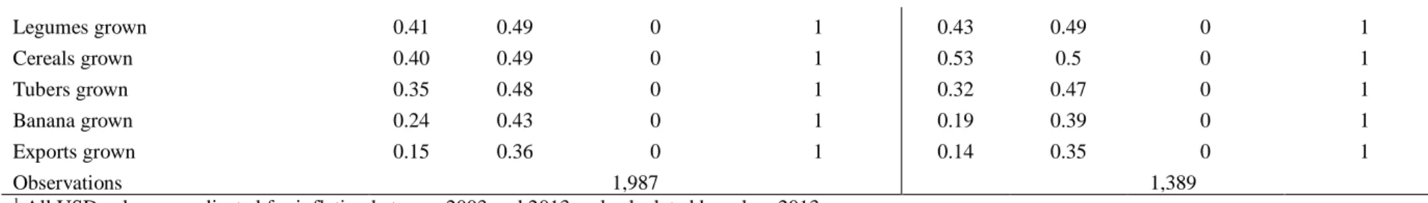
Legumes grown 0.41 0.49 0 1 0.43 0.49 0 1
Cereals grown 0.40 0.49 0 1 0.53 0.5 0 1
Tubers grown 0.35 0.48 0 1 0.32 0.47 0 1
Banana grown 0.24 0.43 0 1 0.19 0.39 0 1
Exports grown 0.15 0.36 0 1 0.14 0.35 0 1
Observations 1,987 1,389
1 All USD values are adjusted for inflation between 2003 and 2013 and calculated based on 2013 average
exchange rates
Table 2.2 Ordinal logistic regression predicting perception of soil fertility (1=poor, 2=average, 3=good)
Stacked 2003 2013
Laboratory Measures
pH 2.172 1.047 3.855
sq(pH) 0.959 1.045 0.885
Organic Matter (%) 1.045+ 1.093*** 0.987
ln(Total Phosphorus) 1.061 0.875 1.530***
Sand (%) 1.006 1.005 1.005
Household Characteristics
Age of Head of HH 1.003 0.995 1.013+
Male Head of HH (0/1) 0.992 0.996 0.922
Formally Educated Head of HH (0/1) 1.001 0.707+ 1.823+
Accessed Agricultural Training (0/1) 1.337* 1.132 1.683*
Household Size 0.99 1.021 0.941
Agriculture primary income source of HH (0/1) 1.121 1.045 1.073
ln(Asset Value)(USD) 1.034 1.03 0.99
ln(Livestock Value) (USD) 1.038 1.035 1.075+
ln(Distance to Local Market)(km) 1.083 1.173* 0.883
ln(Distance to All-Weather Road)(km) 1.002 0.882 1.072
Plot Characteristics
30
Table 2.3 Ordinal logistic regression predicting perception of soil change (1=degraded, 2=no change, 3=improved)
Laboratory Measures
pH 3.455
sq(pH) 0.902
Organic Matter (%) 0.976
ln(Total Phosphorus) 0.954
Sand (%) 1.002
Household Characteristics
Agriculture primary income source of HH (0/1) 0.811
ln(Asset Value)(USD) 1.005
ln(Livestock Value) (USD) 1.037
ln(Plot Size)(ha) 1.047 1.019 1.062
Precipitation(mm) 1.003 1.005 0.989
Slope(%) 0.985 0.995 0.977
Topsoil Depth(cm) 1.345*** 1.386*** 1.451***
Rill Erosion (0/1) 0.683** 0.660** 0.713
Sheet Erosion(0/1) 1.045 0.939 1.243
Year Fixed Effect (2013) 1.126
Constant 39.047 13.886 5.777
Joint Test of Laboratory Measures 18.94** 46.76*** 19.18**
Joint Test of Household Characteristics 12.980 10.43 11.99
Joint Test of Plot Characteristics 61.43*** 58.68*** 36.47***
Observations 3344 1987 1387
*** p<0.001, ** p<0.01, * p<0.05, + p<0.1
Robust standard errors clustered at community level Coefficients reported as odds ratios
31
ln(Distance to Local Market)(km) 1.513+
ln(Distance to All-Weather Road)(km) 0.783
Plot Characteristics
ln(Distance from HH to Plot)(km) 1.023
ln(Plot Size)(ha) 0.836
Precipitation(mm) 0.99
Slope(%) 1.055*
Topsoil Depth(cm) 1.291+
Rill Erosion (0/1) 0.553*
Sheet Erosion(0/1) 1.074
Constant 352689.891
Joint Test of Laboratory Measures 2.000
Joint Test of Household Characteristics 11.380
Joint Test of Plot Characteristics 31.15**
Observations 715
*** p<0.001, ** p<0.01, * p<0.05, + p<0.1
Robust standard errors clustered at community level
Coefficients reported as odds ratios
2003 baseline soil sample measures included but not shown
Cropping types (legumes, cereals, tubers, banana, cash crops), percentage overlap between 2003 and 2013, age, gender, education, and training of head of household included but not shown
District fixed effects included
Table 2.4 Multilevel random effects regression predicting plot productivity/ha (USD)
Stacked 2003 2013
Laboratory Measures
pH 1.873** 1.858+ -0.712
sq(pH) -0.131* -0.111 0.060
Organic Matter (%) -0.005 -0.009 0.000
ln(Total Phosphorus) 0.032 0.063 0.084+
32
Perception 0.246*** 0.247** 0.238**
Household Characteristics
Age of Head of HH -0.002 -0.003 -0.000
Male Head of HH (0/1) 0.242** 0.259* 0.182*
Formally Educated Head of HH (0/1) -0.130 -0.036 -0.079
Accessed Agricultural Training (0/1) 0.122+ 0.073 0.148*
Household Size -0.002 -0.012 -0.002
Agriculture primary income source of HH (0/1) 0.058 0.124 -0.039
ln(Asset Value)(USD) 0.084** 0.101* 0.090**
ln(Livestock Value) (USD) 0.025+ 0.032 0.024+
ln(Distance to Local Market)(km) -0.065+ -0.020 -0.094+
ln(Distance to All-Weather Road)(km) 0.085* 0.059 0.070
Plot Characteristics
ln(Distance from HH to Plot)(km) 0.078*** 0.066* 0.029
ln(Plot Size)(ha) 0.721*** - -0.700*** 0.630***
-Precipitation(mm) 0.001 0.004 -0.002
Slope(%) -0.014* -0.020* 0.001
Topsoil Depth(cm) 0.128*** 0.103** 0.058
Rill Erosion (0/1) -0.016 0.054 -0.167*
Sheet Erosion(0/1) 0.211** 0.347** 0.038
Year Fixed Effect (2013) 1.585***
Constant -6.777** -8.247** 5.748*
Joint Test of Laboratory Measures 36.54*** 41.14*** 5.44
Joint Test of Household Characteristics 46.46*** 20.20* 39.94***
Joint Test of Plot Characteristics 2256.2** 1965.44*** 463.5***
Observations 3,344 1,965 1,379
Number of groups 122 121 104
*** p<0.001, ** p<0.01, * p<0.05, + p<0.1
CHAPTER 3: WHAT DRIVES ENVIRONMENTAL MIGRANTS? LONGITUDINAL EVIDENCE FROM UGANDA
Introduction
In recent years, environmental change has been linked with a range of harmful potential social outcomes including agricultural failure, health problems, and increased poverty
(Bilsborrow, 2009; IPCC, 2014). Through these and other mechanisms, climate change and environmental degradation have subsequently been posited as primary drivers of largescale involuntary human migration and mobility (Myers, 2002). The general premise of this scenario is that, as a result of climate and environmental issues, millions of people worldwide will be forced to permanently move long distances for survival (Warner, Hamza, Oliver-Smith, Renaud, & Julca, 2010).
disasters are more likely to induce local, temporary moves than long-distance permanent migrations (Gray, 2009, 2011; Massey, Axinn, & Ghimire, 2010).
Our analysis builds upon a growing body of literature that has explored environmental effects on migration by linking large-sample socio-demographic data with gridded environmental datasets. Through this approach, studies have been able to examine the broader relationships between different environmental factors and types of human mobility. Past researchers have explored the effects of natural disasters (Gray and Mueller, 2012a; Gray et al., 2014; Halliday, 2006), climate variability (Bohra-mishra et al., 2014; Gray and Mueller, 2012b; Henry et al., 2004; Hunter et al., 2013; Jennings and Gray, 2014; Mueller et al., 2014; Nawrotzki and Bakhtsiyarava, 2016), and land degradation (Gray, 2011; Gray & Bilsborrow, 2014; Hunter et al., 2014) on permanent and long and short term temporary migration. At present, however, very few of these studies have simultaneously explored a number of different environmental and climatic drivers (Gray & Bilsborrow, 2013) along with a range of different migration outcomes (Gray, 2011). Thus, due to the range of contexts, scales, types of migration, and time periods captured by these analyses, it is difficult to discern whether the range of outcomes found in previous studies are based on actual variation in processes or differences in data and methods (Gray & Bilsborrow, 2013).
temporary migration while short term heat shocks are associated with low male temporary
migration, suggesting that temporary migration is enabled by higher agricultural productivity and lower demand for on-farm labor. Extended periods of heat are associated with an increase in male permanent migration, however, indicating that households may eventually be pushed through necessity to send permanent migrants. Our study suggests that rising temperatures may be the most threatening aspect of global climate change and that climate change migration is likely to be a gendered process.
Background
Researchers have long theorized that most migration events fall somewhere on a
spectrum ranging from completely voluntary moves to forced displacements (Hugo, 1996). The most straightforward ‘forced’ migrations are those induced by a natural disaster while the most clear ‘voluntary’ migrations are those involving a wealthy household choosing where and when to relocate. Most migration events fall somewhere between ‘forced’ and ‘voluntary’. Households may be ‘pushed’ to send migrants by economic or environmental stress, or individuals may be ‘pulled’ to migrate for educational or employment opportunities (Black, Adger, et al., 2011). These ‘push’ and ‘pull’ factors are mediated and moderated by a host of socio-economic, demographic, and environmental characteristics including the age, education, and gender of a potential migrant, household resource availability, and community accessibility of migration destinations.
et al., 2010). Through rural-rural or rural-urban seasonal labor migration, household members can provide households with remittance income and lessen household food stress (Black,
Bennett, Thomas, & Beddington, 2011; Ellis, 2000). In contrast, permanent migrations are those wherein an individual or household leaves an area without intent to return (Hunter et al., 2014). Permanent migrations may be due to family formation or result from necessity when an area ceases to provide sufficient livelihood opportunities (Ellis, 2000).
In the rural developing world, migration is often associated with environmental stress through these livelihood pathways. Opportunities for in situ off-farm livelihoods are often limited in these contexts and many households are heavily dependent on natural resource-based livelihoods (e.g. agriculture, harvesting forest products). These livelihood contexts lead to high exposure, high sensitivity, and low adaptive capacity, resulting in households highly vulnerable to shifts in the environmental landscape (Hugo, 1996; Hunter, 2005; McLeman & Smit, 2006).
Environmental changes can take many forms but soil degradation, deforestation, and climate variability are considered particularly concerning across the developing world,
Lambin, 2003; Van der Geest, 2011) while others have found that households with poor soil fertility may lack the resources necessary to support migration (Gray, 2011).
As with soil degradation, deforestation concerns stem largely from the context of rapid population growth, which in turn has led to increased demand for forest products. Between 2000 and 2012, Sub-Saharan Africa experienced high rates of forest loss (Hansen et al., 2013). Apart from the clear environmental issues related to loss of carbon sequestration and biodiversity from deforestation, forest product collection and harvesting of forest for timber, sometimes illegally, is a staple of many rural livelihoods in Sub-Saharan Africa (Jagger, Shively, & Arinaitwe, 2012). Loss of forest can weaken this aspect of rural livelihood strategies, potentially contributing to a heavier reliance on agriculture, livestock production, nonfarm diversification strategies, and migration. In Ghana, for example, deforestation has been cited as a driving factor of rural-urban migration (Carr, 2005).
These environmental concerns are only exacerbated by the current and projected impacts of climate change on Sub-Saharan Africa. According to the Intergovernmental Panel on Climate Change’s latest assessment, Sub-Saharan Africa is likely to experience increased temperatures and increased spatial and temporal variability of precipitation (IPCC, 2014). This constellation of climate effects alone has the potential to wreak havoc on crop seasonality, agricultural
broadly shown to increase migration, but these effects vary across contexts (Gray & Mueller, 2012; Gray & Wise, 2016).
In reviewing the literature, it is clear that environmental shifts in Sub-Saharan Africa are potential drivers of migration, though these effects vary substantial across countries. It is less clear whether these conflicting findings are based on substantive differences in context or
methodological variations. Few of these studies consider more than one environmental factor and many data sources are unable to disaggregate temporary and permanent migrations, though they clearly are largely driven by different processes. Further, few of these studies consider different motivations (e.g. labor, marriage) for migration, or the individual (e.g. gender) characteristics that may shape these processes. Responding to these gap in the literature, our study examines the effect of precipitation, temperature, soil fertility, and forest cover on temporary and permanent migration in Uganda, stratifying by migration characteristics and controlling for a range of socio-demographic household and individual factors.
Data Collection
The Ugandan context
agriculture declined from 52% to 15% between 1992 and 2010, nearly 80% of the population is currently employed in agriculture (Uganda Bureau of Statistics, 2014).
Since the pre-colonial period, migration has been a staple of Ugandan livelihood
strategies. Many of these migration flows are seasonal and cyclical, with individuals temporarily migrating for education or employment opportunities in cotton and coffee plantations or mines (Black, Crush, Peberdy, & Ammassari, 2006). As part of a household livelihood strategy, these cyclical migration flows can provide remittances to rural households while also lessening individual food insecurity by decreasing household size (Ellis, 2000). Ugandans also engage in rural to urban migration. In 2011, the total population growth rate of Uganda was 3.4% while the urban population growth rate was 5.4%, suggesting that the difference arises from rural-urban migration rather than exorbitantly higher rates of natural increase (Mukwaya, Bamutaze,
Mugarura, & Benson, 2011). Finally, though forced displacement due to attacks from the Lord’s Resistance Army (LRA) continues to plague northwestern Uganda (Internal Displacement Monitoring Centre, 2017), none of the communities chosen for our study have experienced forced displacement due to conflict between 2003 and 2013.
Socio-environmental data
(see Appendix F). In 2013, a team of researchers from IFPRI, NARL, the University of North Carolina at Chapel Hill (UNC-CH), Cornell University, Purdue University, and Brown University carried out the second wave of this survey.
In both waves, Ugandan enumerators conducted surveys and gathered spatial data at the household, plot, and community levels, and collected plot-level soil samples for laboratory soil analysis (see Appendix 1 for soil sampling and analysis procedures; see Appendix 2 for spatial data procedures).Survey enumerators were able to return to 727 of the 849 households
successfully interviewed in 2003 during the 2013 follow-up (see Appendix 3 for differences between tracked and lost households). Further, original household members who had formed their own households in between surveys were tracked down and interviewed about their new households if they were still living within their original parish. In total, survey enumerators were able to collect household and plot survey and soils data from 831 households in 2013. In
addition, soil samples were successfully collected and laboratory analyzed from 1,965 plots in 2003 and 1,389 plots in 2013.
We combine these survey data with high-resolution climate and forest cover data. Our measures of temperature and precipitation data are extracted for each community from the University of East Anglia Climatic Research Unit’s (CRU) time-series 3.24. CRU is a monthly global dataset with a resolution of 0.5 degrees (approximately 50 km at the equator) generated through interpolation of data from a network of over 4,000 weather stations worldwide
(UEACRU et al., 2013). CRU data are broadly considered to be a reliable source of climate measures in Africa (Zhang, Kornich, & Holmgren, 2013). Further, the precipitation information produced by CRU is viewed as more spatially and temporally realistic than other climate
of forest cover is generated using the Global Forest Change 2000-2013 dataset, which has a resolution of 1 arc-second per pixel (approximately 30 meters at the equator) (Hansen et al., 2013). Specifically, we draw upon the 2000 and 2010 Landsat reanalysis images, which provide spatially explicit information about percentage of tree cover at the pixel level.
Analysis
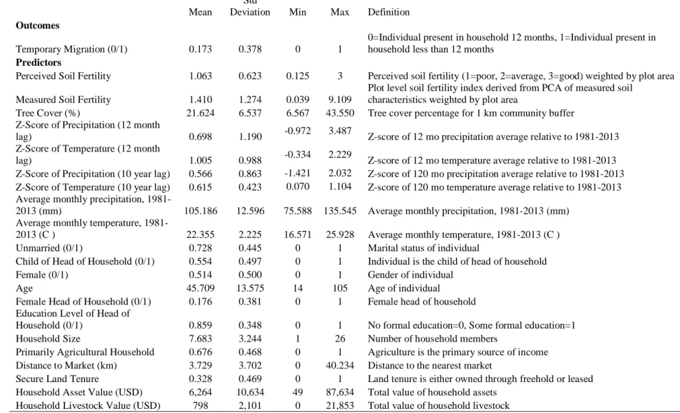
In order to estimate the impact of the environmental predictors on migration, we begin by using the survey data to construct an individual measure of temporary migration and a
household-year measure of permanent migration. Concurrently, we use the survey and soils data to generate our measure of soil fertility and to build a number of controls at the individual and household levels to account for additional potential influences on migration decisions. Following this, we use spatial methods to extract monthly community-level measures of temperature and precipitation as well as measures of forest cover for 2000 and 2010 from high-resolution gridded reanalysis products. Next, we employ a combination of logistic regression, multinomial logistic regression, and discrete time event history analysis to estimate the impact of the climate and environmental predictors on temporary and permanent migration. Finally, we examine the impact of climate and environmental factors on household crop productivity in order to better interpret the findings from our migration analysis.
Migration measures
To examine environmental influences on migration, measures of temporary and
motivation for absence. Household members who were present in the household for less than 12 months are considered to be temporary migrants in this survey. The temporary migration
category is broken down into short and long term temporary migrants by the number of months that a household member is absent from the household. Those who were absent less than 6 months are defined as a short term temporary migrant while those who are absent between 6 and 11 months are defined as long term temporary migrants. Temporary and permanent migrations include both economic (labor) and non-economic migrations. Migration motivations were decomposed into economic and non-economic reasons for migration, with economic reasons being all of those that were related to moving for employment or income generation. Male and female temporary migrations were also examined separately, to assess potential gendered differences in migration patterns (see Table 1 for descriptive statistics).
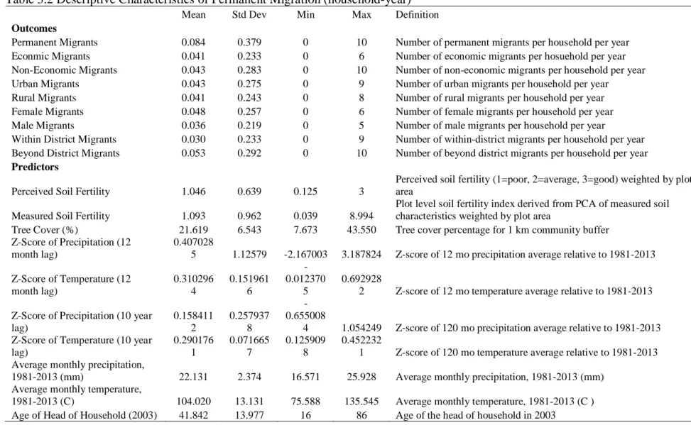
Permanent migrations were measured using a retrospective migration module that was part of the 2013 wave of the survey. This module asked the household respondent to list the individuals who had migrated in the years between 2003 and 2013 as well as the years they had migrated, the migration motivation, whether they moved to a rural or urban destination, and whether their move was local (within district), internal, or international. These data were used to construct a measure of the number of permanent migrants sent from a household each year. This measure was decomposed into measures of number of economic/non-economic migrants, rural/urban migrants, male/female migrants, and within-district/beyond district migrants sent by a household in a given year) (see Table 2 for descriptive statistics).
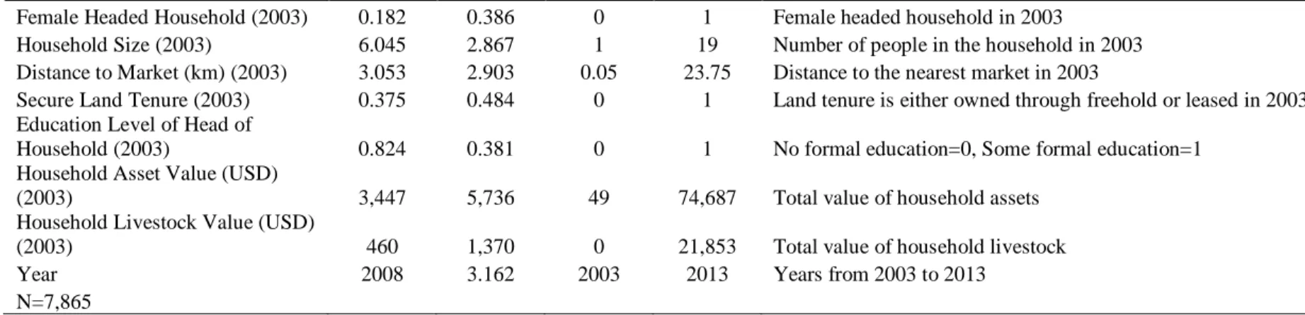
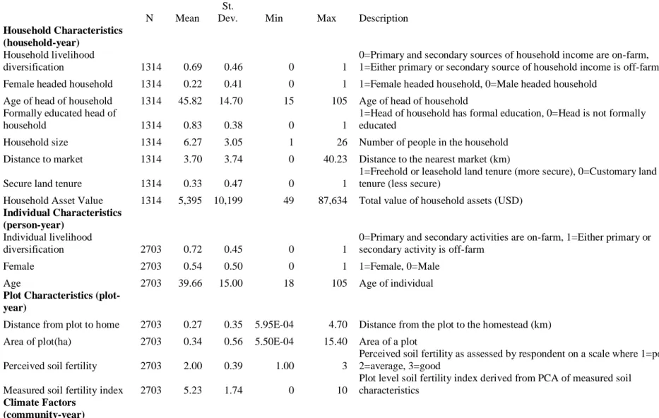
These survey data were also used to generate a standard set of controls that have
household while household level controls include age, gender, and educational level of head of household, household size, household distance to the nearest market, land tenure status of the household, household asset value, and household livestock value (see Tables 1 and 2 for descriptive statistics).
Environmental measures
As previously mentioned, temperature and precipitation values were derived from high-resolution monthly CRU data. For all parts of our analysis, we use z-scores (with 1980-2013 as the period of comparison) to measure temperature and precipitation anomalies. For temporary migration, we generate z scores using 12 and 120 month moving averages starting with the month of survey while for permanent migration we generate z scores using yearly 12 and 120 month moving averages starting with 2003 and continuing on through 2013. We chose to construct 12 month (1 year) and 120 month (10 year) climate anomalies to test for differences between short term coping and long term adaptation to climate shocks, as previous research has shown that these differences can exist (Bohra-mishra et al., 2014; Gray & Wise, 2016).
their plot in reference to the total area of land owned by a household prior to analysis. The results of the analysis demonstrate that greater than 50% of the variance is explained by the first
principal component, meaning that it is a suitable measure of soil fertility. The value of the first principal component, referred to in the analysis as measured soil fertility, was then rescaled to range from 0 to 10. In addition to measured soil fertility, we operationalize soil fertility with area-weighted perceived soil fertility, referred to in the analysis simply as perceived soil fertility. We have chosen to include this subjective measure of soil fertility because previous research has suggested that perceptions can often predict migration patterns more strongly than objective measures (Massey et al., 2010). Further, an analysis of these data examining the relationship between perceived and measured soil fertility found them to be complementary predictors of crop productivity (Call 2017, under review) (see Table 2 for descriptive statistics).
Regression approaches
Logistic regression models were estimated to assess the effects of environmental factors on person-year stacked cross-sectional data for temporary migration while controlling for additional factors. Once the temporary migrations were decomposed into long and short term temporary migrations, economic and noneconomic temporary migrations, and female and male temporary migrants, they were analyzed using multinomial logistic regression models. Using a negative binomial approach, we then estimated the relationship between environmental factors and the yearly number of permanent migrations from a household collected through a
retrospective migration module. As with temporary migration, these permanent migrations were decomposed migration motivation, migration destination, migrant gender, and migration
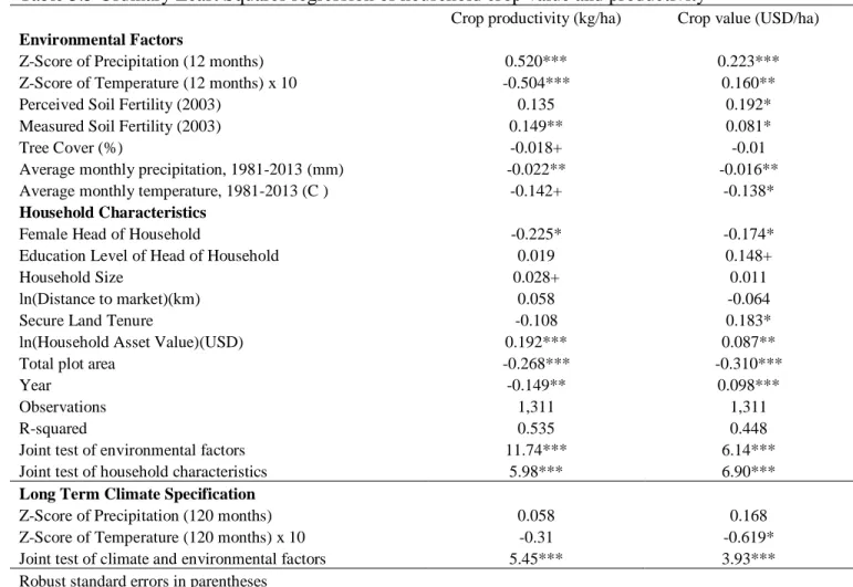
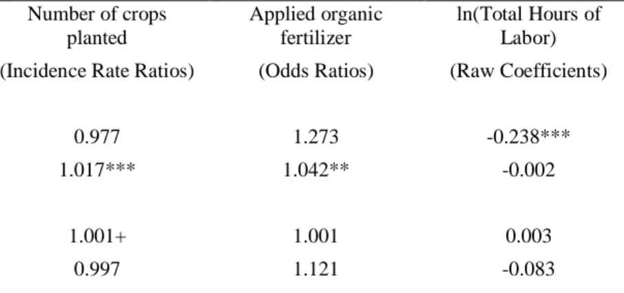
regression was used to investigate the association between environmental and climate factors and crop productivity using stacked cross-sectional data from 2003 and 2013. In all models, district fixed effects are included to adjust for agro-ecological, socio-demographic, and other omitted variable differences between each of the districts. Year fixed effects are included in the stacked temporary migration analyses to account for structural and cultural differences between the two years of data collection. Fixed effects for crop type (e.g. legumes, cash crops, tubers, cereals, banana) were included in the crop productivity analysis to adjust for crop-specific differences in yield and market value. Al models are clustered at the community-levels to adjust for the non-independence of residuals.Values from the logistic regressions are shown as odds ratios while values from the event history analysis are shown as incidence rate ratios, which can be
interpreted like odds ratios. In all regressions, household asset values, household livestock values, and household distance to nearest market are log transformed for normality, as they are highly right-skewed.
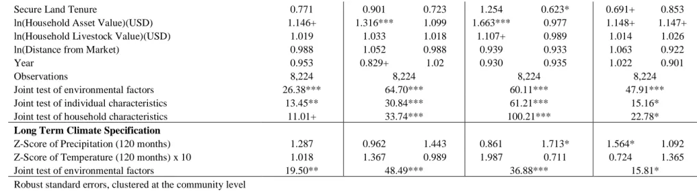
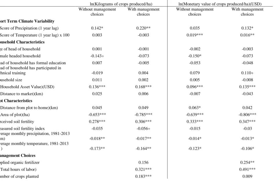
Results and Discussion
Results from the analysis can be found in Tables 3, 4, and 5. Table 3 presents odds ratios of environmental effects on temporary migration while Table 4 presents incidence rate ratios for environmental effects on permanent migration. Table 5 contains the results of our crop
productivity analysis. We will begin by examining the overall significance of the environmental effects jointly and individually before elaborating on each migration subpopulation. We will conclude with a discussion of the results of the household and individual level control variables.