ESSAYS INTRADE AND DEVELOPMENT
Alexander Pearson
A dissertation submitted to the faculty of the University of North Carolina at Chapel Hill in par-tial fulfillment of the requirements for the degree of Doctor of Philosophy in the Department of
Economics.
Chapel Hill 2018
Approved by: Simon Alder
Patrick Conway
Anusha Chari
Lutz Hendricks
c
2018
ABSTRACT
ALEXANDER PEARSON: Essays in Trade and Development. (Under the direction of Simon Alder)
My dissertation focuses on the spatial aspects of trade and development. The first chapter looks at recent improvements in border crossing and port efficiencies in Southern and Eastern Africa to estimate how such trade frictions affect trade flows. I use a general equilibrium gravity model with multiple sectors and trade with the rest of the world in order to capture both direct and indirect effects from border improvements. The reduction of border wait times from an average of 30 hours to 10 is estimated to have increased internal trade by 3.96 billion USD. This amounts to 21% of the total increase in trade between African countries between 2008 and 2014, with inland countries having a greater benefit. I further find an additional 9.46 billion USD increase in internal trade flows when I equalize border wait times to those seen in developed countries.
Amanda, thank you for your constant love and support. You have helped me become a better person in countless ways for which I am forever grateful for.
ACKNOWLEDGMENTS
I would like to thank my advisor, Simon Alder, whose guidance, support and kindness were paramount to my work at the University of North Carolina at Chapel Hill.
TABLE OF CONTENTS
LIST OF TABLES . . . vii
LIST OF FIGURES . . . viii
1 Why Don’t African Countries Trade More With Each Other? The Role of Border Crossings in General Equilibrium . . . 1
1.1 Introduction . . . 1
1.2 Literature Review . . . 3
1.3 Data . . . 5
1.3.1 Multi Modal Transportation . . . 7
1.4 Empirical Analysis . . . 8
1.4.1 Gravity Equation Estimation Results . . . 11
1.4.2 Measure of Combined Transportation Cost . . . 15
1.4.3 Robustness Exercises . . . 16
1.4.4 Limits to Reduced Form Gravity Equations . . . 17
1.5 General Equilibrium Framework . . . 18
1.5.1 Model Setup . . . 18
1.5.2 Model Estimation . . . 22
1.5.3 General Equilibrium Calibration Estimation Results . . . 24
1.6 Counterfactual Analysis . . . 25
1.6.1 No Border Improvements . . . 25
1.6.2 Efficient Border Crossings . . . 27
1.6.3 Ports Like China . . . 27
2 The Effect of Commodity Prices and Mines on Spatial Development: Evidence from Satellite
Data . . . 30
2.1 Introduction . . . 30
2.2 Literature Review . . . 32
2.3 Data . . . 34
2.3.1 Mining Data . . . 34
2.3.2 Administrative Areas . . . 35
2.3.3 Measuring Growth at the Sub-National Level Using Luminosity Data . . . 36
2.3.4 Institutional Data . . . 36
2.4 Empirical Analysis . . . 37
2.4.1 Baseline Specification . . . 37
2.4.2 Multiple Resource Specification . . . 38
2.4.3 Institutional Effects . . . 38
2.4.4 Spillover Effects . . . 39
2.4.5 Benefits to Capitals Versus Mining Areas . . . 40
2.4.6 Institutional Effects on Spillovers . . . 41
2.4.7 Identifying the Spatial Effects of Mines . . . 42
2.5 Results . . . 44
2.5.1 Local Effect of Mining Activity . . . 44
2.5.2 Distributional Effects of Mining Activity . . . 46
2.5.3 The Role of Institutions . . . 47
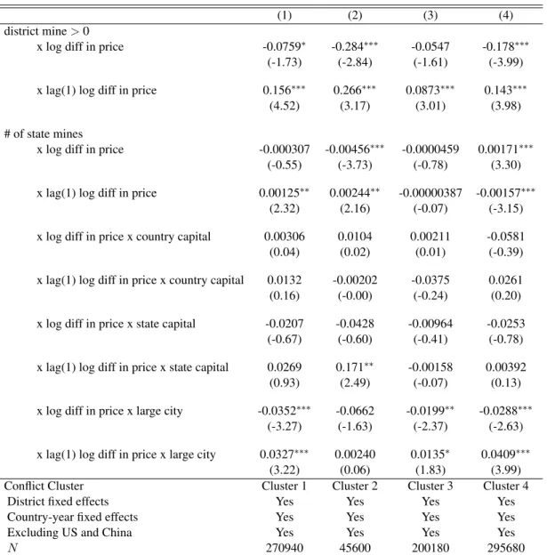
2.5.4 The Role of Conflict . . . 48
2.6 Differences in Revenue Sharing Policies . . . 50
2.7 Conclusion . . . 53
A Appendix for Chapter 1: Why Don’t African Countries Trade More With Each Other? The Role of Border Crossings in General Equilibrium . . . 54
A.2 Model Details . . . 70
A.2.1 Single Sector Setup with Comparative Statics . . . 70
A.2.2 Single Sector Comparative Statics . . . 72
A.2.3 Comparative Statics and Calibration for Multi Sector Model . . . 73
A.2.4 Solving Model for Counterfactuals . . . 75
A.3 Identification . . . 78
A.3.1 Reverse Causality . . . 78
A.3.2 Comparing Calibration Techniques: First Order Approximation versus Solved Model Approach . . . 80
B Appendix for Chapter 2: The Effect of Commodity Prices and Mines on Spatial Develop-ment: Evidence from Satellite Data . . . 83
B.1 Additional Tables . . . 83
B.2 Additional Analysis . . . 96
B.2.1 Asymmetric Effects . . . 96
B.2.2 Alternate Spillover Measure . . . 96
WORKS CITED FOR CHAPTER 1 . . . 99
LIST OF TABLES
1.1 Growth of trade flows from infrastructure changes: No rest of world trade . . . 13
1.2 Growth of trade flows from infrastructure changes: Instrumental variable approach . . . 14
1.3 Growth of trade flows from infrastructure changes using Pseudo Poisson Maximum Likeli-hood estimation . . . 15
1.4 GE single sector results . . . 25
1.5 Percentage point change in trade patterns with no improvements: for internal and foreign trade. Universal gravity model approach . . . 27
2.1 Descriptive Statistics: District Level . . . 35
2.2 Effect of commodity price and resource abundance on light growth . . . 45
2.3 Effect of commodity price and resource abundance on light growth: State wide spillover effects . . . 47
2.4 Effect of commodity price and resource abundance on light growth: Institution groups . . . 49
2.5 Effect of commodity price and resource abundance on light growth: Conflict groups . . . . 51
2.6 Effect of commodity price and resource abundance on light growth: Revenue sharing policy analysis . . . 52
A.1 Descriptive statistics for bilateral trade flows . . . 54
A.2 Proportion of trade for 2008 and 2014 by sector . . . 55
A.3 Dependent Variable: log difference in border wait time . . . 55
A.4 Growth of trade flows from infrastructure changes: Including rest of world trade . . . 56
A.5 Growth of trade flows from infrastructure changes 15 sector case: exogenous border instru-ment sectors 1-5 . . . 56
A.6 Growth of trade flows from infrastructure changes 15 sector case: exogenous border instru-ment sectors 6-10 . . . 57
A.7 Growth of trade flows from infrastructure changes 15 sector case: exogenous border instru-ment sectors 11-15 . . . 57
A.10 Growth of trade flows from infrastructure changes 15 sector case: exogenous border instru-ment, aggregated transportation costs . . . 59
A.11 Estimation results : Time of Trucking on Cost of Trucking . . . 59
A.12 Growth of trade flows from infrastructure changes 15 sector case: exogenous border instru-ment, aggregated transportation costs . . . 60
A.13 Growth of trade flows from infrastructure changes: Constant Routes . . . 60
A.14 Growth of trade flows from infrastructure changes 15 sector case: exogenous border instru-ment, aggregated transportation costs with constant routes . . . 61
A.15 Growth of trade flows from infrastructure changes: Symmetric Border crossings . . . 61
A.16 Growth of trade flows from infrastructure changes: Imports with no supplementation . . . . 62
A.17 Growth of trade flows from infrastructure changes: Exports with no supplementation . . . . 62
A.18 Growth of trade flows from infrastructure changes: PPML estimation with imports and ex-port with no supplementing . . . 63
A.19 Growth of trade flows from infrastructure changes 15 sectors case with 3 year averages . . . 63
A.20 Growth of trade flows from infrastructure changes 15 sectors case with institution interactions 64
A.21 GE multiple sector results . . . 64
A.22 Percentage point change in trade patterns with no improvements. Universal gravity model approach . . . 65
A.23 Percentage point change in trade patterns with 3 hour borders. Universal gravity model approach . . . 65
A.24 Percentage point change in trade patterns with 3 hour borders: for internal and foreign trade. Universal gravity model approach . . . 66
A.25 Percentage point change in trade patterns with China ports. Fixed effects estimation approach 66
A.26 Percentage point change in trade patterns with modern ports. Universal gravity model approach 67
A.27 Percentage point change in trade patterns with modern ports: for internal and foreign trade. Universal gravity model approach . . . 67
A.28 Growth of trade flows from infrastructure changes: Exogenous border instrument . . . 69
A.29 Growth of trade flows from infrastructure changes using Pseudo Poisson Maximum Likeli-hood estimation: Excluding products that use air transport . . . 69
B.1 Effect of commodity price and resource abundance on light growth: long term effects . . . . 83
B.3 Effect of commodity price and resource abundance on light growth: By aluminum, coal and
zinc . . . 85
B.4 Effect of commodity price and resource abundance on light growth: By gold, silver and nickel 86 B.5 Effect of commodity price and resource abundance on light growth: Institutions . . . 87
B.6 Effect of commodity price and resource abundance on light growth: Spillover effects and local effects on cities/capitals . . . 88
B.7 Institution Clusters . . . 89
B.8 Institutional Clusters . . . 90
B.9 Conflict Clusters . . . 91
B.10 Conflict clusters . . . 92
B.11 Effect of commodity price and resource abundance on light growth: Ownership and size of mines . . . 93
B.12 Effect of commodity price and resource abundance on light growth: Size and development state of resources . . . 94
B.13 Effect of commodity price and resource abundance on light growth: Size and development state with lags . . . 95
B.14 Growth of total light from price changes and resource abundance: Aggregated Resource with positive and negative price change measures . . . 97
LIST OF FIGURES
A.1 Estimating the multi-sector gravity constants . . . 68
CHAPTER 1
WHY DON’T AFRICAN COUNTRIES TRADE MORE WITH EACH OTHER? THE ROLE OF BORDER CROSSINGS IN GENERAL EQUILIBRIUM
1.1 Introduction
Although geographically close, countries in Sub-Saharan Africa (SSA) trade relatively little with one another. Intra-regional trade between countries in SSA amounts to 10% of total trade, a much lower per-centage than in other geographical areas.1 Models that account for economic size, geographical distance along with other characteristics such as common language, colonial links and exchange rates, predict trade flows that would be higher than what are observed (World Bank 2009). Furthermore, the Linder Hypothesis (Linder 1961, Bernasconi 2013, Fajgelbaum et al. 2011), which states that countries with similar character-istics, usually measured in the literature by income distributions, will trade more with each other, seems not to apply to countries in SSA.
The low levels of inter-regional trade has not been due to a lack of attention. The benefits of integra-tion, which allows countries to take advantage of economies of scale and to reallocate resources to more productive areas, have been advocated by African leaders and developmental agencies for several decades. This has led to the formation of 14 regional economic communities (RECs), of which each country is a member of at least one, with many countries being a member of several. These RECs have predominantly been focused on reducing the tariffs on goods between the member countries, but with mixed results (World Bank 2012). However, other characteristics of the region, such as poor transportation infrastructure and high non-tariff barriers, can also have a substantial negative impact on the trade flows between countries. For in-stance, in 2008, crossing the border from the Democratic Republic of Congo to Zambia took an average of 96 hours on top of having to drive on roads in poor condition and complete an average of 16 trade documents.
This paper studies this issue by investigating the impact of border frictions, primarily through border wait
1
times, on bilateral trade flows and analyzes their significance to regional integration in a general equilibrium trade model. I focus my attention on two major RECs, the Southern African Development Community (SADC) and the East African Community (EAC), which significantly reduced their border wait times by enacting one-stop border posts (OSBP) between 2008 and 2014.
I use border survey data taken before and after the OSBP were introduced and combine this with various transportation cost variables such as the distribution and conditions of the road network, port efficiencies and product-specific tariff rates. I then analyze the effect of border wait times on bilateral trade flows in two steps. First, I estimate a reduced form gravity equation with importer-sector-year and exporter-sector-year fixed effects using a long difference specification between 2008 and 2014. Taking advantage of the mul-tiple borders that some countries have to cross along their optimal transport route in order to trade, I use an identification strategy that relies on border crossings that are not controlled by the origin or destination country. This allows me to find the direct effects of border wait times on bilateral trade flows. By measuring the change in wait times, this analysis goes beyond the literature that estimates the effects of borders using a dummy variable approach. I find that a 10% wait time decrease for a border that trading partners do not control, yet still have to use, can increase trade between those partners by 3.36%. Furthermore, manufactur-ing and agricultural products saw the largest responses to border wait changes.
Changes in bilateral trade costs can also have important indirect effects on other countries. Therefore the second part of the paper uses a framework that incorporates these additional trade frictions into a general equilibrium gravity trade model developed by Allen et al. (2014) that includes multiple sectors. I calibrate the model using the time variation in the transportation costs and the corresponding trade flows for each trading pair. I then use a series of counterfactuals that show how intra-regional trade was affected by vari-ous improvements to border crossings and ports. For instance, to see how the recent OSBP improvements affected the share of trade between countries in the SADC and EAC, I provide a counterfactual where no border improvements occur. I find that overall trade would be 4.57 billion USD lower each year if the borders were not improved to 2014 levels. With an approximate cost of between 3.5 and 30 million USD, improving border crossing between countries offers a substantial return on investment.2 Furthermore 87%
of those gains were due to increases in trade within the region, suggesting that decreased border wait times
2
spurred economic integration instead of increasing the proportion of foreign trade. I also consider coun-terfactuals that reduce border wait times to those seen in OECD (Organization for Economic Co-operation and Development) countries and improve port efficiencies to the level of the country with the most efficient ports, in terms of costs, which is China. These counterfactuals show that the increased port efficiency and the elimination of wait times at border crossings yield large benefits.
The paper is organized as follows. Section 2 provides a brief overview of the literature. Section 3 cov-ers the relevant data used. Section 4 provides the empirical analysis using reduced form gravity equations. Section 5 describes the general equilibrium trade model, which is then calibrated, and section 6 provides counterfactual border friction scenarios. Section 7 offers conclusions.
1.2 Literature Review
The question of why African countries have such low trade with one another relates to a substantial liter-ature on border effects and their relation to trade flows. The border effect puzzle came to attention with the seminal work of McCallum (1996), who found abnormally large estimates of borders effects of trade flows between the United States and Canadian provinces using a traditional gravity equation. This launched an array of studies that tried to explain these high estimates and provide a theoretical foundation to the border effect.3 Anderson and van Wincoop (2003) provide an explanation for why the McCallum study found sub-stantially overestimated border effects, stating that not accounting for multilateral resistance variables such as remoteness led to omitted variable bias.4 Even accounting for remoteness, Anderson and van Wincoop (2003) still find sizable border effects between Canada and the United States. Analyzing border effects by looking at between and within country trade has the advantage of not requiring any information about the frictions that the border actually causes. However, the effect of this artificial border may have a variety of possible explanations as to why they inhibit trade such as differing regulations, border congestion, infor-mation frictions and heterogeneous substitution of goods. This creates difficulties in explaining how any particular aspect of borders actually affects trade flows between countries.
3
These studies include different regions such as Europe (Nitsch (2000), Pisu and Braconier (2013) Reggiani et al (2014)), US and Japan (Parsley, Wei, 2001), and other regions between America and Canada (Coughlin and Novy (2011) and Gandhi and Duffy (2013) and also accounting for other variables (Hliberry (1999), Wei (1996), Frankel and Wei (1998), Anderson and van Wincoop (2003), Chen (2004), and Millimet and Osang (2007).
4
One way to solve this issue, as done in this paper, is to gather data on border characteristics that relate to transportation costs. In their paper on the six major puzzles of international trade, Obstfeld and Rogoff (2001) transportation costs as a dominant factor in why these puzzles remain unsolved. However, almost all the studies mentioned above use distance and tariffs to account for transportation costs. Although tariff reductions were the major contributor to increased international trade over the last half-century, tariffs have been reduced to negligible levels in many cases. Other costs to transport will thus be more significant in explaining the continuing border effect (Baier and Bergstrand 2001). Although this area of research is rela-tively untouched, a few papers do use other methods to measure transportation costs to account for the border effect. Gandhi and Duffy (2013) use the extra security measures on the Canadian-U.S border to explain the decline in trade share between the two countries. Pisu and Braconier (2013) look at the connectivity of road networks between European countries and see that higher connectivity within countries accounts for 25% of the reduction in trade among countries with borders them. Studies have also tried to apply this gravity equation approach to trade between African countries including Akpan (2014), who looks at the Economic Community of West African States (ECOWAS) and estimates a gravity equation using distance and percent-age of roads paved to account for transportation costs.
U.S incomes.
Finding data on the changes of non-tariff barriers that affect transportation costs can be difficult. There-fore, studies have also looked at the variation in prices of commodity goods due to changes in transportation infrastructure. Sotelo (2015) finds that an average farmer gains 16% in productivity and 4% in welfare due to the paving of existing dirt roads in Peru. Atkin and Donaldson 2014 provide a method of dealing with issues of using the price gap as a means of estimating trade costs and find that within-country trade costs due to log distances are four to five times higher in Ethiopia and Nigeria than they are in the United States.
1.3 Data
In order to capture transportation costs, I first create a transportation network that accounts for the qual-ity of the roads between all countries in the SADC and EAC (16 countries in all). The main data sources are the Center for International Earth Science Information Network (CIESIN) and the African Development Bank Group, which provides details of the road networks in each country of the SADC and EAC for 2010. The data includes information on road types and conditions.
Since there have not been efficiency studies to determine the speeds for certain roads in these countries, I assign an approximated speed for each road given its type and condition. These approximations are calcu-lated by taking roads of similar type and quality from data from the World Bank (2005) in India and Roberts et al (2010) in China. Therefore, I assume that a new paved highway that was in good condition had a speed of 70 km/h. For paved highways in poor or fair condition, a speed value of 40 km/h was assigned. Unpaved dirt or gravel roads have a speed of 25km/h assigned. Locations that did not have any transportation net-works, I assign a speed of 10 km/h to account for potential small unobserved trails.
crossings is the average of low through-traffic crossings as reported by the World Bank (2010). Many border crossings took days to get across with the highest being five days on average. Other borders had very low wait times of a few hours. Many of the surveys also include monetary costs in fees that have to be paid to cross the border. In this transportation network I allow movement only through the official border crossings.
With this transportation network, I then begin to construct transportation costs from each country in my sample to the others. While a number of methods have been used to model transportation costs, Roberts et al. (2012) shows that travel times provide a suitable proxy for overall transport costs. In order to obtain transportation times in 2008 and 2014 from the constructed transport networks, I use a Dijkstra algorithm in ArcGIS to find the shortest travel time between each of the main cities of each country to every other main city in each country. To get the transportation costs to each country the location of the beginning and ending points are important. This is especially true if there are many large cities in one country that are all importing and exporting to other countries, leading to different travel costs for each city. To get around this issue, I take the top three to five cities in each country and find the travel costs to get to every other city in the other countries. Since cities may import or export more due to their relative size I use a weighted average of each city’s travel costs weighted by their development in order to obtain a bilateral transportation cost measure.5 For the main analysis in sections 4 and 5.3, I allow for the optimum route to change between 2008 and 2014 given the changes in border wait times. This leads to some trading partners having changes in their road transportation times even though there were no large changes in the road speeds during this time.6
Bilateral trade flow data was taken from UN Comtrade for the years 2008 and 2014.7I use the two-digit product classification, leading to 97 different product types. I use import data since import data tends to be more accurate than compared to export data due to the fact that imports are more likely to be taxed.8 Some countries did not report trade flows in 2008. For these countries, I use the export data from other countries that did report to approximate their imports. For trade with the rest of the world I combine countries into five
5Since city-level measures of development are incomplete, I proxy for level of development by using the intensity of night time
luminosity.
6
For robustness I also include analysis for when I keep the routes identical in both time periods.
7
Additionally, I use IMF direction of trade (DOT) bilateral trade data to provide robustness checks.
8
groups: North America, 27 countries of the European Union, Asia, South America, and the rest of Africa. Appendix Table A.1 shows the change in trade flows by sector and internal/foreign trade. We see that during this time, trade between other countries in the SADC and EAC saw significant gains compared to trade with foreign regions. This is especially true for the agriculture and manufacturing sectors. Indeed manufacturing goods traded internally accounted for nearly half of overall manufacturing trade in 2014.
Tariff data is obtained from two WTO databases, the Integrated Database and the Consolidated Tariff Schedules. The latter also states whether specific countries have certain trade agreements with each other. If no such trade agreement was listed, then the Most Favored Nations value was used. Incomes and Popu-lations were taken from the World Bank Development Indicators. Distance was constructed the same way as travel times, i.e. taking the distance from the top cities in each country to the other cities in the other countries. Common language, whether the country is landlocked and adjacency are other variables that were used. Institutional variables such as rule of law, regulatory quality, political stability, and corruption were obtained from the Worldwide Governance Indicators.
1.3.1 Multi Modal Transportation
Several papers forgo the inclusion of interactions that are outside of the study area.9 Others incorporate trade with the rest of the world (such as Turner (2015)), but assume sea trade to be constant during the period of analyses. Adding accurate rest-of-world trade and the corresponding costs have the potential to change one’s result significantly. This is even more of a concern in this case study since 85% of total trade is with countries outside the study region.
The largest hurdle to incorporating different modes of transportation inside a general equilibrium model is the problem of providing a unit cost or ad valorem cost that is compatible with each mode. This practice is still in its infancy with no consensus on how it should be done. In southern and eastern Africa, road transportation is the predominant method of transportation, whereas sea trade is mostly used for trading with the rest of the world.10 In order to include the transportation network with the rest of the world, costs
9Donaldson and Hornbeck (2014) allow for trade to take place over water but only to other areas in the U.S. Donaldson (2013)
outlines four areas that can trade internationally within the Indian region for the particular good.
10
pertaining to port usage needed to be acquired. To do this, I used the World Bank’s Doing Business survey which surveys local freight forwarders, customs brokers, and traders in 189 countries. For each country, the survey breaks up the costs for both importing and exporting into domestic transport, border compliance, and documentary compliance. Each country is assumed to import a container of auto parts valued at 50,000 USD and weighing 15 metric tons. Exports are derived from each country’s leading export.11 It is also assumed that the cargo is shipped from the largest city within the respective country. Travel times and costs are also documented from the major city to the nearest border if the country is landlocked or the nearest port if not.
The survey also includes data on the time and costs to go from the primary city to the port or border. This can give us an approximation of per-hour costs for road transportation. Section 4.2 goes over the strategy of combining different modes of transportation together. The monetary value of time, the additional costs at each port pair, and the tariff structure to the rest of the world gives most of the costs that are incurred in transporting goods across borders. One large unknown is the role that road-blocks and bribes play in each country. The data on transport cost to port or border may include these interactions but likely do not report the detailed structure of road block locations or the magnitude of charges at these road blocks. This however affects most studies concerning road transportation in developing countries and until reliable data is available and correctly incorporated into the transportation networks there is little to be done.
1.4 Empirical Analysis
In this section I estimate the effects of border wait times on trade flows using a reduced form gravity equation. Gravity equations have been used extensively to estimate a wide variety of determinants in trade.12 Taking advantage of the border crossing surveys, I will be able to exploit the time variation to determine the effect of border improvements on trade flows. To account for any lag in the response of trade to changes in trade frictions, I conduct a long difference estimation with importer-sector and exporter-sector fixed effects between 2008 and 2014 where all of the surveys and improvements were implemented. Let
∆ lnXijs =µ∆ lnTij +β1∆Zij+γis+δjs+ij (1.1)
whereXijs are trade flows fromitojin sectorS,Tij is the sum of all border waiting times thatiand
jhave to incur to trade with one another andZijis the set of control variables including tariffs, road travel
times and port efficiencies if one of the trading partner is overseas.13
The importer-sector and exporter-sector fixed effectsγis andδjsaccount for the unobservables that are
determinants to trade flows such as productivity, labor and capital prices and institutions. This method also absorbs variables that we observe but that are time and country specific, such as income.14
Ideally the changes in border crossing wait times would come from events that were exogenous to coun-tries decision to trade with one another. In practice, this may not be true. If two councoun-tries expected to trade more with each other in the future, this may lead them to improve their border crossings to allow an easier movement of goods. In this scenario, the goods might have been moved regardless, and the improved border crossings could have little effect and would lead to an upward bias in the estimate forµ. The opposite may also be true. For example, when consumers and firms in each country wish to trade with one another, it may lead to higher protectionist measures from their governments. However, a key characteristic of having many countries in the same region is that, when one country decides to change their border frictions with their neighbor, regardless of their intent, other countries that use the border crossing to get to their other trading partners, now have an exogenous change in their transportation costs. This is due to other countries having very little influence on how the first two countries improve their transportation network. The more thorough approach that I apply here is to use a border or a set of borders in between two non-adjacent trading partnersiandj, as an instrument for the total time cost between the respective trading partners. This subset of border/borders will be correlated to the overall time cost but exogenous toiandj’s unobserved actions to increase trade with one another. Furthermore, these non-adjacent countries account for only 1% of the trade going through such that there is no reverse causality from trade to waiting times since they have little effect on the congestion at these borders.
I therefore use a two-stage least squares estimate with the first stage defined as
13Section 4.2 goes over the case in which the independent variable T is the aggregate transportation friction from roads, ports
and border wait times with various robustness checks.
14
∆ lnTij =α1∆ lnBc+ψi+φj+νij (1.2)
Wherec∈Ωij andΩij is the set of borders thatiandjhave to go through to trade with each other andψi
andφj are the importer and exporter fixed effects. Then we can use this to estimate the main equation by
∆Xijs =β1( ˆα1∆ lnBc+ ˆψi+ ˆφj) + ∆Zij+γis+δjs+ij (1.3)
whereαˆ1∆ lnBc+ ˆψi+ ˆφj = ∆ ln ˆTij is the predicted values from (1.2).
Using an instrumental variable that only accounts for 1-2% of the total trade within the region raises potential concerns. First the types of goods traded may be very different from the overall population of trade flows. However, as we can see in Appendix Table A.2, the proportions of traded goods among sectors are relatively similar to non-adjacent trade.
Another potential concern is the endogeneity of trade flows to border times due to congestion. All else equal, an increase in trade flows between two countries would increase the traffic and the number of trucks that would have to wait in line to go through the border resulting in longer wait times. This would lead to the wrong conclusion that higher wait times leads to higher volumes of trade. To check for reverse causality, I look at the effects of trade flows on border wait times by creating a measure for trade flows that is indepen-dent of policy decisions and investment made during that time period. This can be found in appendix B.1. However as mentioned before, when limiting my sample to non-adjacent countries, this endogenous effect would be mitigated, since they account for only 1% of what is traded on the studied transportation network. Therefore, any changes in trade flows between these countries will have a marginal effect on overall wait times.
One important characteristics of this study is the quasi-random nature with which trading partners re-ceive their trade frictions through border wait times due to their lack of control over non-adjacent borders. However, if changes in border wait times are highly correlated between borders, it would suggest that there are non-observables that could affect both border wait times and trading behavior among countries, leading to biased estimates on border wait times. To check for this, I run an unbalanced panel regression of the change in the border wait time of one of the trading partner’s own borders, on the average time change of borders not controlled by either trading partner along their trade route. Since each country belongs to many trade routes I also control for this by using country fixed effects. Appendix Table A.3 shows close to zero correlation between borders controlled by trading partners and borders not controlled along their trade routes with a t score of -.03.
Estimating equation 1.1 assumes that each product traded will be affected equally by border wait times. However, a more likely scenario is that some products, such as agricultural goods, will be affected differently than other goods such as copper which may not be as time sensitive. To see how trade costs are affected in a per sector basis, I estimate
∆ lnXijs =µs∆ lnTij+β1∆Zsij+γis+δsj +sij (1.4)
wheresnow denotes the type of industry the traded good comes from. As mentioned in section 3, the trade flow data is categorized by 97 products that can be aggregated into 15 sectors, which I did in order to make the importer-sector-year and exporter-sector-year fixed effect matrices small enough to be computa-tionally feasible.15
1.4.1 Gravity Equation Estimation Results
To see how border wait times affect trade flows following the specification in equation 1.1, I begin with the 15-sector case excluding the rest of the world. This baseline result is shown in Table 1.1. Columns 1 to 3 show both adjacent and non-adjacent trading partners with column 3 including the full specification. As we see, a 10% decrease in border wait times is expected to increase trade flows by 3.64%. However, when taking into account the proximity of trading partners using distance, the effects of border wait times are
15
smaller when partners are farther away. That is, the trading partners that were farther than the median dis-tance away from each other saw only a 1.2% increase in trade for every 10% decrease in border wait times. This may be due to information frictions that make it more difficult for distant countries to take advantage of lower trade barriers. When I disregard trade between adjacent countries within the study region there is still a statistically significant negative relationship although with a lower magnitude which is consistent with the findings in column 3 since, by construction, non-adjacent countries are farther away.
The estimates found for the effects of changes in the aggregate tariff rate on the change of trade flows are reported to be positive. There are a number of potential ways to explain this counter-intuitive result. First, by 2008 tariffs were eliminated for all non-sensitive products. Once the minimum requirements were met for the non-sensitive products, products on the sensitive list were required to be reduced as well. Many of these particular products took longer to become duty free therefore, for these sensitive products, it could be the case that the products expected not to be imported as often, were the easier products to reduce tariff rates on. Additionally, the products that were expected to increase in imports in the future could give governments an incentive to maintain tariffs at high levels for those products. Second, Pelikan and Brockmeier (2008) show how using weighted aggregate tariffs can lead to endogeneity issues that underestimate the effects of tariffs. As tariff rates increase and the number of imports subsequently goes down, the actual change in tariff rates will be smaller due to the weight of that product decreasing. Finally, many of the tariffs still in place may be over products that report zero imports. This eliminates the observation from the standard regression along with the information that high tariffs reduced the imports of that product (to zero).
Appendix Table A.4 incorporates trade with the rest of the world and includes a control for port costs. Changes in border wait times show similar effects when looking at southern and eastern African trading partners and trade that occurs with the rest of the world. Changes in port costs during this time period corre-lated positively with trade flows. A potential reason could be that higher trade volumes put larger demands on ports than they have capacity for, which could raise costs.
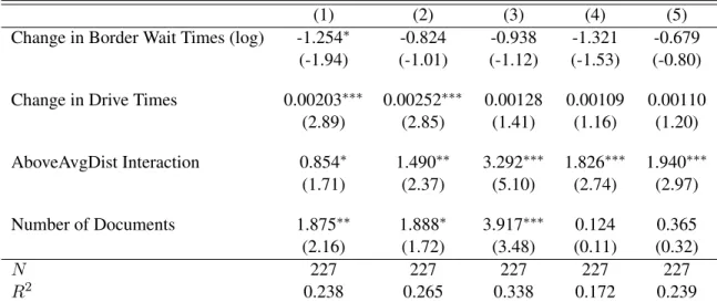
Table 1.1: Growth of trade flows from infrastructure changes: No rest of world trade
(1) (2) (3) (4) (5) (6)
Change in Border Wait Times (log) -0.184∗ -0.364∗∗∗ -0.898∗∗∗ -0.161∗ -0.189∗∗ -0.394∗∗∗ (-1.71) (-3.42) (-6.97) (-1.75) (-2.00) (-2.99) Change in Drive Times 0.00229∗∗∗ 0.00183∗∗∗ 0.000299 0.000277
(12.29) (8.31) (1.24) (1.00)
AboveAvgDist Interaction 0.778∗∗∗ 0.237∗
(5.94) (1.76)
Change in Tariffs 0.456∗∗∗ 0.531∗∗∗
(8.76) (10.78)
Number of Documents -0.461 -0.154
(-1.41) (-0.49)
Adjacency/Non Adjacency Both Both Both Non adjacent Non adjacent Non adjacent
N 3360 3360 3330 2505 2505 2490
R2 0.210 0.250 0.277 0.276 0.277 0.317
The dependent variable is growth in imports from 2008 to 2014 aggregated to 15 different sectors. Regressions are controlled for importer-year-sector and exporter-year-sector fixed effects with robust standard errors. t values reported in parenthesis. Significance levels are: * 0.10, ** 0.05, *** 0.01.
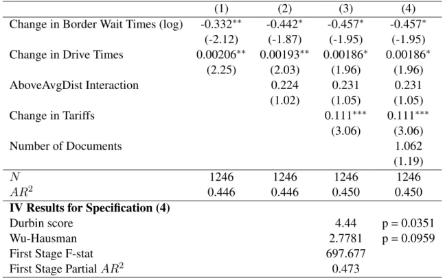
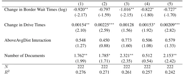
flows due to a 10% decrease in wait times. To see if an instrumental variable approach is needed, I conduct a Durbin test and obtain a value of 4.44, which rejects the null hypothesis that the variables in the OLS regression alone are exogenous and shows it as correct to treat border wait times as an endogenous variable. In checking for weak instruments, I find an F-statistic of 697.67, with a threshold of 16.38 meaning I can reject the null hypothesis that the instrument is weak.
Table 1.2: Growth of trade flows from infrastructure changes: Instrumental variable approach
(1) (2) (3) (4)
Change in Border Wait Times (log) -0.332∗∗ -0.442∗ -0.457∗ -0.457∗
(-2.12) (-1.87) (-1.95) (-1.95)
Change in Drive Times 0.00206∗∗ 0.00193∗∗ 0.00186∗ 0.00186∗
(2.25) (2.03) (1.96) (1.96)
AboveAvgDist Interaction 0.224 0.231 0.231
(1.02) (1.05) (1.05)
Change in Tariffs 0.111∗∗∗ 0.111∗∗∗
(3.06) (3.06)
Number of Documents 1.062
(1.19)
N 1246 1246 1246 1246
AR2 0.446 0.446 0.450 0.450
IV Results for Specification (4)
Durbin score 4.44 p = 0.0351
Wu-Hausman 2.7781 p = 0.0959
First Stage F-stat 697.677
First Stage PartialAR2 0.473
The dependent variable is growth in imports from 2008 to 2014 aggregated to 15 different sectors. Regressions are controlled for importer-sector and exporter-sector fixed effects. t values reported in parenthesis. Significance levels are: * 0.10, ** 0.05, *** 0.01.
in trade flows due to a 10% decrease in border wait times when trading partners were below median distance apart, but also a 1.96% increase for trading partners that were above median distance from each other.
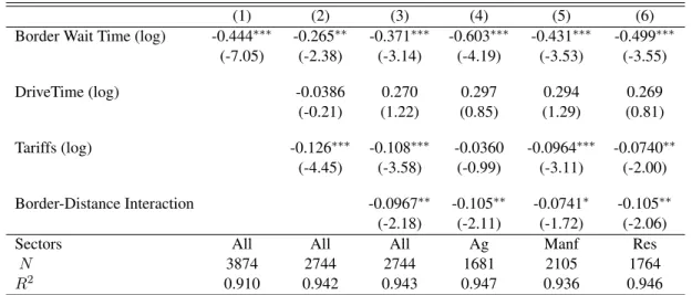
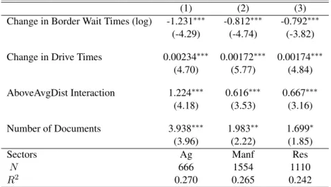
Pseudo Poisson Maximum Likelihood Estimator
Table 1.3: Growth of trade flows from infrastructure changes using Pseudo Poisson Maximum Likelihood estimation
(1) (2) (3) (4) (5) (6)
Border Wait Time (log) -0.444∗∗∗ -0.265∗∗ -0.371∗∗∗ -0.603∗∗∗ -0.431∗∗∗ -0.499∗∗∗
(-7.05) (-2.38) (-3.14) (-4.19) (-3.53) (-3.55)
DriveTime (log) -0.0386 0.270 0.297 0.294 0.269
(-0.21) (1.22) (0.85) (1.29) (0.81)
Tariffs (log) -0.126∗∗∗ -0.108∗∗∗ -0.0360 -0.0964∗∗∗ -0.0740∗∗
(-4.45) (-3.58) (-0.99) (-3.11) (-2.00)
Border-Distance Interaction -0.0967∗∗ -0.105∗∗ -0.0741∗ -0.105∗∗
(-2.18) (-2.11) (-1.72) (-2.06)
Sectors All All All Ag Manf Res
N 3874 2744 2744 1681 2105 1764
R2 0.910 0.942 0.943 0.947 0.936 0.946
The dependent variable is growth in imports from 2008 to 2014 aggregated to 15 different sectors. All variables are calculated by a 3 year average. Regressions are controlled for importer-year-sector and exporter-year-sector fixed effects. t values reported in parenthesis. Significance levels are: * 0.10, ** 0.05, *** 0.01.
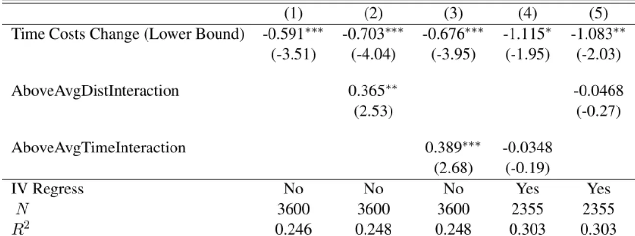
1.4.2 Measure of Combined Transportation Cost
Another method used in this paper is to create a transportation friction measure that incorporates the changes in driving costs, border wait time costs and port costs. One benefit of this method is that it reduces the number of parameters needed to calibrate the general equilibrium trade model. An additional benefit comes from being able to analyze multiple modes of transportation using monetary values. Converting bor-der and road friction measures into a monetary value however, requires information on the cost of time in transit. Two different strategies are used in this paper to create this transportation cost measure as explained below. It is important to note that increasing the monetary value of the wait time is equivalent to increasing the weight of the importance of overall change in aggregate transportation costs.
Ad-Valorem Time Costs
in both tables again use non-adjacent borders as an instrument for the aggregate trade cost measure. We see that changes in the value assigned to each hour of waiting does not significantly change the coefficient of interest. I find that a 1% decrease in the cost of transportation between trading partners leads to a 1.16% increase in trade.
Trucking Survey Costs Strategy
Another method for obtaining ad valorem costs would be to use the World Bank Doing Business survey which includes the time and costs required to go from the primary city to the port or border. This can give us an approximation of per hour costs for road transportation which I can then use to get the average marginal cost of an additional hour of driving. Appendix Table A.11 shows that every hour adds on average an ad-ditional 27 USD to transport costs, which is approximately the midpoint of the ad-valorem tariff estimates found by Hummels and Schaur 2013. Appendix Table A.12 shows similar magnitudes to those found in Appendix Tables A.9 and A.10 which were derived from the ad valorem estimate.
1.4.3 Robustness Exercises Optimal Routes
One assumption made when constructing border wait time measures between bilateral trading partners is that the optimal path is allowed to change given new border times between the countries. To check whether this assumption will affect my results, I re-estimate Table 1.1 but hold constant the route used for travel. Appendix Table A.13 shows the new results and Appendix Table A.14 uses the aggregated transport friction measure holding the optimal route constant. In both instances the border friction measure remains negative and close to what is found when allowing the route to change. This is most likely due to the fact that many routes used in 2008 were still the optimal routes in 2014.
Symmetric versus Non-Symmetric Border Crossings
surprising as border wait times for each direction are similar.
Trade Flow Measures
When import data are not available between two trading partners but export data are available from the other reporter, I assume that the amount of trade that occurred was equal to the export data of the other reporter. Appendix Table A.16 uses data only for imports and records zero even if the respective trading partner’s export data contradicts the import data. Appendix Table A.17 exclusively uses export data. Since more zeros are recorded, Appendix Table A.18 uses the PPML estimator with import data exclusively which allows for zero trade flows. Appendix Table A.19 then takes the average of the importer’s data and the ex-porter’s data with little change in the estimates. I assume that goods are traded by road or by sea. However, 10% of African trade also takes place by air (Hummels and Schaur 2013). To account for this, I re-estimate the reduced form model but exclude products that are more likely to be transported by air and obtain similar results.16
Institutions
To analyze the effects that institutional characteristics have on how trade reacts to travel costs, I include interaction effects for four different variables; regulation quality, rule of law, political corruption, and polit-ical stability. Appendix Table A.20 shows that better regulatory quality, rule of law, politpolit-ical stability and less corruption increases the amount of trade between partners when travel costs are decreased.
1.4.4 Limits to Reduced Form Gravity Equations
Although the fixed effects gravity estimator is one of the most common methods for estimating gravity equations there remains one main limitation. Estimates of the border wait time variables only show the direct effects on trade and do not take into account potential trade dispersion. The fixed effects gravity estimator is able to control for this multilateral resistance term but cannot estimate the indirect effects of changes in trade frictions on trade flows. This is a concern when conducting counterfactuals since the trade between two trading partners not only depends on the changes in transport frictions between themselves, but also of other trading partners. In the following section, I therefore use a general equilibrium trade model in order to undertake counterfactuals.
16
1.5 General Equilibrium Framework
A large number of microfounded general equilibrium trade models provide gravity equations for trade flows. The first was the Armington model with intermediate inputs first used by Anderson (1979). Krugman (1980) derived a gravity equation using monopolistic competition and homogeneous firms and intermediate inputs while Meltiz (2003) used heterogeneous firms. Eaton and Kortum (2003) used a Ricardian perfect competition model. Several other papers have extended these workhorse models, But these models face difficulties in guaranteeing uniqueness and characterizing comparative statics, often using sub-optimal as-sumptions to attempt both. Allen, Arkolakis and Takahashi (2014) provide a universal gravity model that nests these other models and allows for uniqueness in equilibrium and closed-form comparative statics with minimal assumptions.
1.5.1 Model Setup
In this section I define a general equilibrium trade model created by Allen et al (2014) allowing for multiple sectors.17
Multi-Sector Model
Let the world be comprised of a setS∈(1, . . . , N)of locations. These locations can either be countries or smaller administrative areas. For each location,Yidenotes the gross income andXij the value of location
j’s imports from locationi. Trading between the locations is hampered by a corresponding trade friction represented byKij >0. This represents the costs associated with trading between the two locations, such
as distance, time, and tariffs.
I include multiple sectors as non- tariff barriers and poor infrastructure may affect traded goods differ-ently . For instance, large wait times at each border may make it difficult to transport a variety of agricultural goods due to spoilage. Similarly, manufactured goods may need a variety of complex machines which re-quires the speedy imports of crucial parts to prevent production disruptions due to broken parts. Waiting weeks instead of days for these items may make it difficult to even set up manufacturing in the first place. To account for this I extend the gravity model to include three sectors, agriculture, manufacturing and resource
17
extraction. Again, using work done by Allen et al. (2014) lets∈ {M, A, R}be the set of sectors.
Next, I define, as in Allen et al (2014), (γi) and (δj) as the exporting and importing capacity
respec-tively; this accounts for the microfounded characteristics found in modern trade models, such as wages, prices, productivities, and labor endowments. These two variables are solved endogenously within the gen-eral equilibrium model, allowing us to make fewer assumptions of the underlying mechanisms that many of the seminal trade models focus on while still providing the same outcome. Allen et al (2014) show that four conditions, described below, must be met in this framework in order to obtain the general equilibrium outcomes found in many of the current workhorse trade models.
Condition 1: For any countryi∈Sandj ∈S, the value of aggregate bilateral trade flows is given by
Xijs =Kijs(γi)(δjs). (1.5)
Here, the importer shifters are equalized through each sector. This would be the case if there were no frictions in the labor market in country i, which is assumed here. Ks
ij is interpreted as sector specific trade
frictions letting different commodities have different costs for transport.
The next two conditions are concerned with assumptions of goods market clearing and trade balance that are made in almost all trade models. Specifically,
Condition 2: For any locationi∈S
X
j
Xj,is =BisYi. (1.6)
That is, the total sum of all purchases from all locations, including its own location, is equal to their income share for that sector for all locations. Next, we have
Condition 3: For any locationi∈S
X
s X
j
That is all exports, including the “exports” to their own location, must equal to their income. Although common in the trade literature, this condition rarely holds for countries. Allen et al (2014) addresses this concern and provides a strategy to account for unbalanced trade that will be included in estimation and the counterfactual analysis.
The universal gravity model also assumes a log-linear parametric relationship between gross income and the exporting and importing shifters:
Condition 4: For any locationi∈S
Yi =Biγiα
Y
s
(δis)θs
β
(1.8)
whereα∈IR,β ∈IRθs ∈IRare the gravity constants andBi >0is an (exogenous) location specific
shifter.18 These gravity constants control the response income has on the importing and exporting shifters. In section 5.2, I estimate (α,β, andθs) to allow for the analysis of counterfactual scenarios.
The last condition pins down the equilibrium trade flows by normalizing gross incomes, taking advan-tage of Walras’s law. Finally,
Condition 5: World income equals to one
X
i
Yi = 1. (1.9)
Multi-Sector Comparative Statics
To see how trade frictions affect trade flows and welfare in the model, I take advantage of the work done by Allen et al (2014) who derive comparative statics for the importer and exporter shifters. It is easy then to show the general equilibrium effects for trade and welfare at any location given a change in bilateral trade frictions between any two locations.
18In the Armington model (Armington 1969)Biwould be characterized by population and total factor of productivity for country
The addition of multiple sectors follows the same method as the single sector case above.19The appendix describes the construction of the multi sector comparative statics in detail. It is now possible to have a change in transportation frictions in a specific sector between two countries affect trade between any other country pair and sector. Specifically:
∂γl
∂Kijs =X
s
ij(A+l,i+A
+
l,N+j)−c s ij and ∂δs 0 l ∂Ks ij
=Xijs(A+
(s0N+l),i+A
+
(s0N+l),N+j)−c s ij
whereA+is a(N +SN)×2N matrix and the Moore pseudo inverse to the matrix
A= (α−1)Y βθ1Y −X
1 . . . βθ
sY −Xs
αY −XT βθ1Y −E1 . . . βθsY −Es !
where Y is aN×N diagonal matrix whoseithdiagonal is equal toYi,Esis aN ×N diagonal matrix
who’sithdiagonal is equal to
Eis=X
j
Kjis exp{yj}exp{zi}
or location i’s total expenditure on goods in sector s.XandXsare the total and sector specificN ×N trade matrices respectively. Again,csij pins these values down due to our assumption of condition 5 which states that world income equals one.20
Therefore the effect of a change in transportation frictions for sector s between countries i and j on trade of sectors0from k to l is:
19
The construction of the comparative statics for the single sector model can be found in the online appendix of Allen et al. (2014)
20Specifically:
csij≡
1
YW(α+βP
s0θs0)
Xijs
X
l
Yl(α(A+l,i+A
+
l,N+j) +
X
s0
β(A+
(s0N+l),i+A
+
∂ln ˆXs 0
kl
∂ln ˆKijs = ∂lnγj ∂lnKs ij + ∂lnδ s0 k
∂lnKs ij
=Xijs(A+l,i+A+l,N+j) + (A+
(s0N+l),i+A
+
(s0N+l),N+j))−2c s ij
and income changes for country l is defined by.
∂lnYl
∂lnKijs =α ∂lnγl
∂lnKijs +β
X
s0
θs 0 ∂lnδs
0
l
∂lnKijs =
Xij×(α(A+l,i+A
+
N+l,j+c s ij) +β
X
s0
θs 0
(A+
(s0N+l),i+A
+
(s0N+l),N+j+c s ij)
1.5.2 Model Estimation
Section 5.1 described a model in which for any given α, β,θs, income shiftersBsi and trade frictions
Ks
ijt, a unique general equilibrium could be solved by a set of endogenous import and exporter shifters.
This subsection will address the estimation ofα,β and a trade cost parameterµusing the trade flow and travel time data, which allows for the opportunity of counterfactuals and welfare analysis in section 6. I use the method in Allen et al (2014) which takes advantage of the general equilibrium structure of the model. The approach calculates the importer and exporter shifters directly from the model and predicts the corresponding trade flows. It then estimates the gravity constants and trade cost parameterµby taking the least squared errors between the observed change in trade costs and the predicted change.
(α∗, β∗, θ∗1, . . . , θs∗, µ1∗, . . . , µs∗) =arg min
α,β∈IR,µ∈IRS X s X i X j
ln ˆXijsobserved−ln ˆXijspredicted2. (1.10)
As in Allen et al (2014) the method used to calibrate(α∗, β∗, θ1∗, . . . , θ∗s, µ1∗, . . . , µs∗)is through a grid search. A computationally intensive strategy would be to solve the model to obtainXˆs
ij
predicted
for each it-eration. To simplify the estimation procedure, I follow Allen et al (2014) and take first order approximations to bothln ˆγiandln ˆδjssuch that
(α∗, β∗, θ∗1, . . . , θs∗, µ1∗, . . . , µs∗) =arg min
X s X i X j
ln ˆXijso−Tˆ0s
ijµ−ln ˆγi T µˆ ;α, β, θ
−X
s
ln ˆδs
j T µˆ ;α, β, θ 2
(1.11)
where
ln ˆδs j T µˆ
≈X s0 X k X l
∂ln ˆδs j
∂ln ˆKkls0 ˆ
Tklsµs (1.12)
and
ln ˆγi T µˆ ≈X s0 X k X l
∂ln ˆγi
∂ln ˆKkls0 ˆ
Tklsµs. (1.13)
I calibrate the set of parameters in two steps. First, I estimate the set of optimal trade parametersµs∗. It can be shown that equation 1.11 can be written as
µ(α, β, θ1, . . . , θs) =
D(α, β) ˆT0 (D(α, β) ˆT
−1
D(α, β) ˆT)0yˆ (1.14)
whereTˆdenotes aSN2×M vector whosehi+j(N −1)iis the1×M vectorTˆ0s
ij,D(α, β)is the
SN2×N2matrix withhi+j(N−1), k+l(N−1)irepresenting∂lnX s ij
∂Ks
kl , andyˆdenotes theN
2×1vector
whosehi+j(N −1)irow islnXˆijso.
Therefore for anyα, β, θ1, . . . , θs,µscan be estimated using ordinary least squares on the general
equi-librium transformed explanatory variableTˆsGE ij :
ln ˆXijs = ( ˆTsGE
ij )0µs+sij (1.15)
where
ˆ TsGE
ij = X s0 X k X l
∂ln ˆXs ij
∂ln ˆKkls0 ˆ Tkls
and
∂ln ˆXs 0
ij
∂ln ˆKkls = ∂lnγi ∂lnKs kl + ∂lnδ s0 j
The second step is to find the gravity constantsα, β, θ1, . . . , θswhich minimize the total squared errors.
As shown in Allen et al. (2014) this can be written as
(α∗, β∗, θ1∗, . . . , θ∗s) =
arg min
α,β∈IRyˆ
I−Tˆ
D(α, β) ˆT0
(D(α, β) ˆT −1
D(α, β) ˆT)0
ˆ
y. (1.16)
Using a three-sector version requires solving five parameters. I perform a grid search to limit the con-trol space then, taking the set of parameters, perform a random search around those values to calibrate the parameters.
This method does use approximations to the fully solved model approach in order to obtain the cali-brated parameters. Appendix B.2 compares both methods using Monte Carlo simulations and finds that the approximation approach provides similar results to the fully solved model approach but in a fraction of the time.
1.5.3 General Equilibrium Calibration Estimation Results
elasticity value is converted to a value that corresponds with the universal gravity model, and Row 4 shows values found in Alvarez and Lucas (2007). The explanatory power in values found in other papers appears to be low when applied to the SADC and EAC. This may be due to developing countries reacting differently to transportation changes than developed countries,from where these other gravity constants were estimated.
Table 1.4: GE single sector results
Type
alpha
beta
µ
StdEr
R
2Own Calibration
-23.00
-1.40
-0.62
0.0154
0.0819
AAT Calibration
-30.20
-27.90
-2.36
0.4454
0.0089
EK
-3.85
-3.04
-0.10
0.0790
0.0001
AL
-0.67
-0.33
-5.76
3.3252
0.0008
Coefficients forµrepresent the estimated coefficients of the general equilibrium estimation given various values of the gravity constants. AAT Calibration represents the alpha and beta values calibrated from Allen et al (2014), EK are values found in Eaton and Kortum (2002) and AL are values found in Alvarez and Lucas (2007).
When looking at a three-sector case and using the calibrated values forαandβfound in the single sector model, we see in Appendix Table A.21 large gains in the explanatory power of the data in the manufacturing sector but less in agriculture and resource extraction. All three sectors have negative and significant coef-ficients with manufacturing being of the largest magnitude. Figure A.1 shows the R-squared values of the general equilibrium estimation over combinations of different parameters. We see that there are clear local maxima with a smooth increase in R-sqaured to the calibrated parameter values.
1.6 Counterfactual Analysis
1.6.1 No Border Improvements
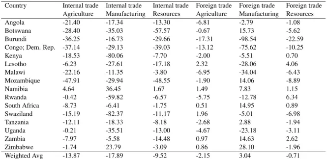
Appendix Table A.22 illustrates the general equilibrium effects on trade from assuming that no border improvements were made between 2008 and 2014 and that border wait times were that of 2008 levels. We see in the agriculture sector, taking a weighted average with respect to countries’ income, that trade would be negatively affected by 12.85 percentage points of the growth of internal trade during that period. This implies that instead of the actual 49.3% increase in agricultural trade during this period, it would be esti-mated to be 36.45% if no border improvements were made.
Table 1.5: Percentage point change in trade patterns with no improvements: for internal and foreign trade. Universal gravity model approach
Country Internal trade Internal trade Internal trade Foreign trade Foreign trade Foreign trade Agriculture Manufacturing Resources Agriculture Manufacturing Resources
Angola -21.40 -17.34 -13.30 -6.81 -2.79 -1.08
Botswana -28.40 -35.03 -57.57 -0.67 15.73 -5.62
Burundi -36.25 -16.73 -29.66 -17.31 -98.54 -22.59 Congo; Dem. Rep. -37.14 -29.13 -39.03 -13.12 -75.62 -10.25
Kenya -18.53 -80.06 -7.70 -2.00 -5.51 0.70
Lesotho -6.23 -27.61 -17.18 2.32 -28.06 4.06
Malawi -22.16 -11.35 -3.80 -6.95 -34.04 -6.43
Mozambique -47.91 -29.94 -48.55 -1.90 14.06 -8.89
Namibia 4.64 36.45 1.67 1.49 7.83 1.15
Rwanda -0.42 -59.82 -6.57 -5.75 -12.78 6.34
South Africa -8.73 -6.41 -1.75 0.51 14.95 0.89
Swaziland -15.19 -82.37 -11.17 1.96 -5.01 -6.98
Tanzania -12.11 -18.33 -8.18 -2.68 2.88 -1.94
Uganda -0.21 -35.51 -13.00 -4.67 -23.18 -3.11
Zambia -7.97 -5.58 -14.48 0.97 14.63 2.62
Zimbabwe -1.74 23.79 -3.09 0.86 28.10 -1.96
Weighted Avg -13.87 -17.89 -9.52 -2.15 3.04 -0.71 Table shows the percentage point difference in the growth of trade flows between the counter-factual scenario of no border improvements and the observed growth in trade from 2008 to 2014.
1.6.2 Efficient Border Crossings
Next, I create a hypothetical scenario in which border waiting times are reduced to 3-hours, similar to that between OECD countries who have established border crossings. Appendix Tables A.23 and A.24 show overall percentage point changes to trade expected from having no borders. This scenario would lead to agricultural trade growth of 60.44% between 2008 and 2014 instead of the actual 49.3%. Trade in man-ufacturing products would see smaller increases with an added 4.32% over the time period with resource trade seeing an additional 9.2% increase. Splitting up trade between internal trade and foreign trade shows that internal trade would significantly increase, particularly in manufacturing products, while foreign trade would stay relevantly constant or even decrease.
1.6.3 Ports Like China
stand to benefit most. Agricultural products would see the least increase in trade with the rest of the world.
Using the universal gravity model, Appendix Tables A.26 and A.27 show similarities among the benefits due to improved ports, with manufacturing seeing the largest gains at 6.03%. Agriculture and resource trade would improve 2.9% and 2.0% respectively. Breaking up trade by exports to the rest of the world, we see large increases in manufacturing (7.6%) and agriculture (3.5%) with little effect on resource trade (0.6%). Unlike with the reduced form counterfactual, here we can begin to look at the effects of port conditions on trade between SADC and EAC countries. On average, the effects of increased port efficiency would be negligible. However, some countries could see moderate effects. Zimbabwe, for instance, would see a 1.2% decrease in resource exports to other countries in the SADC and EAC.
1.7 Conclusion
It has been argued previously that insufficient transportation infrastructure is one of the main compo-nents in limiting trade and, consequently, growth within developing countries. This is particularly true in Africa where many landlocked, remote or low population density countries have to trade with large within and cross-border transportation frictions. This topic also concerns the facilitation of regional integration, particularly through large-scale investments by governments and NGOs to strengthen domestic trade and development. However the usual interdependence of transportation infrastructure, trade and development make it difficult to determine the actual effects that additional investments in transportation infrastructure would have on integration, trade and thus development.
Furthermore, the effects of transportation infrastructure such as roads, ports, and borders on trade flows have been empirically difficult to study due to the dichotomy between countries who have large transporta-tion infrastructure projects but sparse trade flow data, and the countries who have ample trade flow data, but little time variation in their transportation infrastructure over data available time periods. This paper begins to bridge this gap by looking at a multi-country region that has significantly reduced trade costs due to investments in border and port infrastructure in a relatively short period.
CHAPTER 2
THE EFFECT OF COMMODITY PRICES AND MINES ON SPATIAL DEVELOPMENT: EVIDENCE FROM SATELLITE DATA
2.1 Introduction
The growth of large economies like China can have a significant impact on resource abundant countries due to their increasing demand for raw materials that are used to build manufactured goods and large-scale infrastructure projects. For instance, iron ore production tripled between 1992 and 2013, and at the same time, real prices went from 33 USD per dry metric ton (dmtu) in 1992 to 151 USD/dmtu in 2008 before coming down again to 127 USD/dmtu in 2012. Local and national governments that are endowed with an abundance of resources are naturally interested in the regional effects that large commodity price increases will bring. However, whether resource abundance fosters economic development or leads to a resource curse, particularly at a subnational level, is still being debated with no clear consensus.1
This paper provides a new approach to measuring the effects of resource abundance and mining activity on economic development, by exploiting both between and within-country variation, a task that has been difficult due to data constraints. Looking at district level growth and district-specific resource abundance gives insights on where the effects are being felt within the country. In addition to this, looking at over 100 countries then allows for the control of country- and time-specific non-observables, which cannot be done when studying a single country. This allows me not only to determine whether mining districts benefit or not from the mining activity, but also determine which regions in the country are benefiting from the additional revenues at a multi-country level.
Since income data are rarely collected at a subnational level for many countries that are of interest, I use night-time luminosity data from 1992 to 2013, which has been demonstrated to be an adequate alternative to
1
measuring GDP growth when other data is not available (Henderson et al. 2012). In order to quantify the re-source abundance of a district, I use spatial data from the United States Geological Survey (USGS) that has surveyed 305,000 different resource locations worldwide documenting size, type of resource, operational activity and ownership. Using exogenous world pricing data from the World Bank Commodity Market Out-look’s (CMO) dataset, I then estimate the interaction effects of prices and resource abundance on yearly night-time luminosity. Controlling for country-year and district fixed effects, I find that districts with high mining activity tend to grow more slowly than other districts after an initial price increase. However, subse-quent periods show an increase in economic activity within the mining district from the initial price increase for up to five years. A one standard deviation in a price increase leads to an estimated .95 percentage points slower growth for the mining districts for the initial year. However, mining districts see an average of .92 percentage points faster growth in development for the following 4 years after the initial price increase. Taking advantage of the spatial nature of the data, I measure the spillover effects of mining and resource abundant locations on other locations. I find that districts adjacent to mining areas and large cities located within the same state saw similar responses to world price changes as the mining districts, suggesting that cities in resource-rich states depend, to a certain degree, on mining activity in the state for additional growth.
I then determine the role of institutional characteristics and conflict on both the impact on mining dis-tricts and the distributional effects that mining locations have on their states from exogenous world prices. I find that low corruption and high rule of law mitigate the slow growth seen initially and accelerates the growth in subsequent years when world prices increase. In addition, higher levels of external conflict also increased the long-term development of these districts. To analyze the role of institutional characteristics on the distribution of development due to mining activity within a state, I estimate separate responses for four groups of countries that represent different institutional qualities by using a clustering method for bu-reaucratic quality, corruption and rule of law measures.2 I find that countries that have higher bureaucratic quality, low corruption and higher rule of law distribute the effects of mining activity throughout the state. Countries that exhibit weak institutional characteristics see state administrative capitals grow faster than average when world prices increase. I conduct a similar analysis using three conflict measures: internal conflict, external conflict and ethnic tensions. I find that countries with high internal conflict and ethnic tension, but low levels of external conflict see districts within mining states have negative spillover effects
2