Statistical inferences for correlated observations : prediction and estimation

(1)

Statistical Inferences for Correlated Observations: Prediction

and Estimation

by Xuanyao He

A dissertation submitted to the faculty of the University of North Carolina at Chapel Hill in partial fulfillment of the requirements for the degree of Doctor of Philosophy in the Department of Statistics and Operations Research.

Chapel Hill 2009

Approved by:

Richard L. Smith, Advisor

Zhengyuan Zhu, Advisor

Edward Carlstein, Committee Member

Joseph G. Ibrahim, Committee Member

(2)

c

2009

Xuanyao He

(3)

ABSTRACT

XUANYAO HE: Statistical Inferences for Correlated Observations: Prediction and Estimation.

(Under the direction of Richard L. Smith and Zhengyuan Zhu)

(4)

top-ics and data-driven methods on the shrinkage estimation for covariance matrices are discussed. We also consider a model with semi-parametric covariance matrix, which includes both a para-metric and an unstructured part. For this model, we derive a plug-in method for parameter estimation, and also consider how the mean and variance of a kriging predictor are affected if the true matrix V is replaced by an approximation ˆV. We consider a preliminary estimator for the unstructured error, a linear combination of the sample covariance and the diagonal estimator, and we find that in the case of exponential covariance structure (for both simulation and asymptotic results), this estimator performs better than the sample covariance matrix by comparing the mean square errors of their resulting regression coefficient estimators. In the future, we plan to derive some theoretical proofs and more simulation studies.

(5)

ACKNOWLEDGEMENTS

I am deeply indebted to my advisors, Professor Richard L. Smith and Professor Zhengyuan Zhu. They led me into the current research field in Statistics. They helped me in learning a lot of knowledge in Statistics, for instance, the Laplace method, the statistical methods in Bayesian data analysis and Spatial Modeling. From them, I improved myself a lot in getting motivated from real problems, in formulating scientific problems, in developing novel methods and related theoretical justifications to solve those problems, etc. Thanks to their stimulating suggestions, encouragement and complete support through all my time and research at Chapel Hill.

(6)

and Multivariate Analysis, which is taught by Prof. Smith as well, inspired me to study the asymptotic comparison of REML and Bayesian predictive procedures to the AR model, which is very important in data analysis. We find some interesting priors in the model with temporally correlated error. In developing the asymptotic comparison for different predictive densities with correlated data, Professor Zhu also gave me a lot of help in formulating the theoretical properties, and in organizing the simulation results, etc. One of his courses, Spatial Statistics introduced basic concepts about some important spatial models, and kriging. The essential part of the course, inspires me to consider application with respect to models with spatially correlated errors (see 3), and also to investigate the shrinkage estimation for a temporally independent, spatially dependent model (4).

I would like to express my gratitude to my committee members, Professor Edward Carl-stein, Professor Yufeng Liu and Professor Joseph Ibrahim, who gave me their full support in completing this thesis. From the course I audited, Bayesian Statistics taught by Professor Ibrahim, I learned a lot of background knowledge and basic concepts of Bayesian statistics. Professor Carlstein raised really good questions during my proposal presentation, and I input more necessary background materials to explain the use of REML in our work, for estimation of variance parameters. In addition, Professor Carlstein is a great mentor in terms of teaching. He guided me in becoming a good teacher throughout the undergraduate courses I have taught while at Chapel Hill. Professor Liu always encourages me and gives me many inspiring sugges-tions for my research. The discussions I had with all of them helped me to better understand the problems I was studying and helped me make a progress.

(7)

me constant supports in many ways. I also enjoyed my four semesters as a Research Assistant, giving me opportunities to read papers, formulate problems and build my own research career. Everything is charming at Chapel Hill.

For the chapter 2, the author gratefully thanks to the reviewers of JASA for their helpful comments and constructive suggestions related to the second-order approximation.

(8)

List of Figures

2.1 Asymptotic Comparisons of Bayesian and REML-based densities . . . 33

2.2 Asymptotic Comparison for the Improper Prior . . . 34

2.3 Simulation Results . . . 38

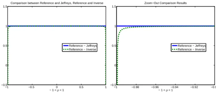
3.1 Asymptotic Comparisons within the Temporal AR(1) Model . . . 53

3.2 Comparison between different priors . . . 54

3.3 Simulation Results for Temporal AR(1) Model . . . 58

3.4 Asymptotic Comparisons within Spatial AR(1) Model . . . 63

3.5 Simulation Results for Spatial AR(1) Model . . . 65

4.1 MSE( ˆφ): Theoretical and Simulation Results for RandomR . . . 86

4.2 MSE(ˆρ): Theoretical and Simulation Results for RandomR . . . 87

4.3 MSE( ˆφ): Theoretical and Simulation Results for Exponential R . . . 88

4.4 MSE(ˆρ): Theoretical and Simulation Results for Exponential R . . . 89

4.5 MSE( ˆφ): Theoretical and Simulation Results for LRDR . . . 90

(12)

Chapter 1 Introduction

(13)

agree well with the asymptotic result, when sample size is moderately large. Chapter 4 studies the impact of different covariance matrix estimations onto parameter estimation and kriging prediction. In contrast to the structured covariance matrix in Chapter 2, a more complicated covariance matrix is assumed, that is, a semi-parametric one which includes both a structured and an unstructured measurement error part. We derive some preliminary results for the “plug-in” covariance parameter estimation, kriging predictor and prediction error. A brief summary of the three parts is given in Chapter 5.

1.1 Asymptotic Comparison of Predictive Densities for

Depen-dent Observations

(14)

freedom in estimating the mean and also produces unbiased estimating equations for the vari-ance parameters) and Bayesian predictive densities with some objective priors. Since the KL divergence of two densities is usually intractable, we derive a higher order Laplace expansion of the KL divergence, and define the notion of “second-order KL REML-dominant” to com-pare predictive distributions using the Laplace approximation. A prior on θ is second-order KL REML-dominant if the REML based estimative distribution is no better than the Bayesian predictive distribution under this prior for allθ, in the sense that the leading term of the second order Laplace expansion of their differences for KL divergences is positive. We provide explicit conditions for second-order KL REML-dominance (see page 23 - 24, Section 2.3.3). In addi-tion, for a specific mixed effect model, we show that the Jeffreys prior is not second-order KL REML-dominant, while an alternative family of improper priors is (see page 28 - 29, Section 2.4.2). To our knowledge, this is the first one of such result for the predictive distribution of

Z, which is dependent onY. Simulation studies match well to the theoretical result. This part was one of the winners of the 2008 student paper awards of American Statistical Association (ASA), Section of Bayesian Analysis, and has been submitted for publication.

1.2 Applications with respect to the AR(1) models

Chapter 3 focuses on an intensive exploration with respect to another correlation structure, by the theoretical methods in Chapter 2. Here we consider two important correlated structure: (1) Temporal AR(p) case; (2) Spatial AR(p) case. Thep-th order autoregressive (AR(p)) model is one of the most important models in time series analysis. It consists of the data_{yt}, satisfying

(15)

the predictive density of the AR(1) model with unknownσ2 and ρ (which is a1 when p = 1), utilizing the criterion of expected K-L divergence, which we propose in Chapter 2. We also point out that the reference prior is superior to the other two candidate ones with respect to the second-order asymptotic approximation. A related work by Tanaka and Komaki (2005) focused on the Bayesian estimation of the spectral density of the AR(2) model and proposed a superharmonic prior as a noninformative prior. They also considered the more general case, the autoregressive moving average (ARMA) model, focusing on the Bayesian estimation of an unknown spectral density in the ARMA model. They first showed that in the i.i.d. cases, the Bayesian spectral densities based on a superharmonic prior asymptotically dominate those based on the Jeffreys prior, using the asymptotic expansion of the risk difference related to expectation of KL divergence. Actually the stationary Gaussian processes are getting close to the i.i.d. cases as the sample size becomes large, and they obtained the asymptotic expansion of the Bayesian spectral density for the ARMA model, which could be written in the differential-geometrical quantities as in the i.i.d. cases. Finally they obtained the corresponding result in the ARMA model. However, our work directly compares different predictive densities instead of the spectral densities, for the case of AR(1) model.

(16)

General definition of the AR(1) model and the necessary notations for Fisher Information Matrix calculation are briefly reviewed in this chapter. Within this framework, we compare different Bayesian predictive densities and REML plug-in density, based on the expected KL divergence, as proposed in Chapter 2. We provide the asymptotic second-order expression of the differences between their expected KL divergences. In Section 3.3.3 and 3.4.3, we apply this approach to AR(1) models, for both time series and spatial structure, respectively. We consider three candidate priors: the Jeffreys prior, the reference prior and the inverse reference prior. Asymptotically, all the three priors perform quite well as compared to the REML-plug in density. In particular, we prove that the reference prior dominates the other two priors. Berger and Yang (1994) also recommended the reference prior, when comparing it with the Jeffereys prior and the uniform prior (which results in MLE estimator) based on another criterion, the MSE of the resulting estimator. In Section 3.3.4 and 3.4.4, we perform numerical simulation for the AR(1) time series and spatial process, illustrating that the asymptotic results hold, when the sample size is moderately large. Some concluding work can be seen in Section 3.5.

1.3 Parameter Estimation and Prediction with Errors in

Co-variances

(17)

in order to obtain related statistical inferences. In Chapter 4, we assume that the covariance matrix of given data contains two parts: some known function of the unknown parameterθ, and the measurement errorR, which is not parametrically constrained. We consider two problems about this model:

(1) Plug-in estimators of θ, by using sample covariance S or a liner shrinkage estimator ˆRν =

νS+(1₋ν)S∗_{, ν} _∈_[0_,_{1], where}_S∗ _{is the diagonal estimator of}_R_{, in the restricted log-likelihood}

function, whereν is an adjustable tuning parameter that represents shrinkage intensity.

(2) How the kriging performance will be affected, when the true covariance matrix is Ktt but we replace it by ˆKtt =Ktt(ˆθ,Rˆ) (see page 67 in Section 4.1 for definition of K) to derive the likelihood equations.

For problem (1), we suppose θ is a vector and θi is the ith element, and we can show that the estimation bias, ˆθi₋θi depends on the first and the second order moments of the first order derivative of the plug-in restricted log-likelihood function and the first order moment of the second order derivative, where “plug-in” means replacing R by ˆR whenever R appears in the definition of these functions or derivatives. Obviously this needs specification for estimation methods of the covariance matrix. As a starting point, we consider a model with an exponential covariance function K and R simultaneously, where R is set to be random, exponential or long range dependence, respectively (see page 78 - 80 in Section 4.3.2). From both theoretical and simulation results, we find that certain linear combination of the sample covariance and the diagonal estimator will result in much smaller mean squared error (MSE) of the plug-in REML estimator ˆθ, given the tuning parameter ν∗_{, which is the optimal value of} _ν _∈ ₍₀_,_{1). We will}

(18)

of empirical kriging predictor. In the future, we plan to get the asymptotic expression of the MSPE, similar to what we have done for problem (1). The next step is to simulate some data and check the effect of different estimators of R on the empirical MSPE.

1.4 Summary

(19)

Chapter 2 Asymptotic Comparison of Predictive

Densities for Dependent Observations

This chapter studies Bayesian predictive densities based on different priors and frequentist plug-in type predictive densities when the predicted variables are dependent on the observations. Average Kullback-Leibler divergence to the true predictive density is used to measure the performance of different inference procedures. The notion of second-order KL dominance is introduced, and an explicit condition for a prior to be second-order KL dominant is given using an asymptotic expansion. As an example, we show theoretically that for mixed effects models, the Bayesian predictive density with prior from a particular improper prior family dominates the performance of REML plug-in density, while the Jeffreys prior is not always superior to the REML approach. Simulation studies are included which show good agreement with the asymptotic results for moderate sample size.

2.1 Introduction

(20)

is the parameter, and Z be another random variable with distribution also parameterized by

θ. Y and Z may be dependent for time series or spatial data, and we would like to predict Z

based on observation Y. In principle, we would like to know the distribution of Z conditional on Y. This is usually characterized by a point predictor and a prediction interval in the frequentist framework, and good prediction means both an accurate point predictor and a narrow prediction interval with correct coverage probability. Alternatively, one can take a decision-theoretic approach and define a loss function between the true conditional density

g(z_|y, θ) and the predictive density ˆg(z_|y). A common measure of discrepancy between two density functionsg and ˆgis the Kullback-Leibler (KL) divergence:

D(g(z_|y, θ),gˆ(z_|y)) =

Z

g(z_|y, θ) logg(z_g(z_ˆ |y,θ)_|_y) dz.

To compare two predictive densities ˜g1 and ˜g2, one can look at the expected difference of KL divergence

Z

{D(g,g˜1)−D(g,˜g2)}f(y;θ)dy. (2.1)

(21)

(22)

2.1.1 Background for Restricted log-likelihood estimation Method

Consider a general linear mixed model

Y =Xβ+Zb+ǫ,

where X and Z are specified design matrices, β is a vector of fixed effect coefficients, b and ǫ

are random, mean zero, and Gaussian if necessary. Usually we can think of b being constant over subjects, ǫ as independent between subjects, possibly correlated within subjects. Let θ

denote free parameters in the variance specification.

We observe n r.v.sY. Once the structure of errors is fully specified, and Cov(b, ǫ) = 0, we have

Y _∼N(Xβ, V(θ)) (2.2)

V(θ) = Var(ǫ) +ZVar(b)ZT. (2.3)

For mixed models, the covariance matrix V is a function of a q-dimensional parameter θ, and is assumed to be positive definite for θ in a neighborhood of the true value. Any estimation or prediction procedure proceeds only if variances and covariances among the observations are known or, more often, after they have been estimated.

(23)

be biased downwards in a linear model), REML corrects this problem by using the likelihood of a set of residual contrasts and is generally considered superior. In other words, REML is often preferred to maximum likelihood estimation as a method of estimating covariance parameters in linear models because it takes account of the loss of degrees of freedom in estimating the mean and produces unbiased estimating equations for the variance parameters.

The restricted or residual maximum likelihood (REML) method was proposed by Thompson (1962), as a way of estimating dispersion parameters associated with linear models. Numer-ous authors have given overviews on REML, e.g.Patterson and Thompson (1971) introduced restricted maximum likelihood estimation (REML) as a method of estimating variance compo-nents in the context of unbalanced incomplete block designs. Surveys of REML can be found in articles of Harville (1977), Khuri and Sahai (1985), and Robinson (1987), and in the book by Searle et al. (1992). Alternative and more general derivations of REML were given by Harville (1974), Cooper and Thompson (1977) and Verbyla (1990). In all of these the restricted like-lihood is presented as the marginal likelike-lihood of the error contrasts. Or it can be regarded as modified profile likelihood in Barndorff-Nielsenn (1983). Some other areas in which REML has been used include the following: estimating smoothing parameters in penalized estimation Wahba (1990) (see Speed (1991) for related discussions); the estimation of parameters in ARMA processes and other time series in the presence of fixed effects (Cooper and Thompson (1977) and Azzalini (1984)); REML estimation in spatial models (Green (1985) and Gleeson and Cullis (1987)); or the analysis of longitudinal data in Laird and Ware (1982); and REML estimation in empirical Bayes smoothing of the census undercount in Cressie (1992). Therefore, in our work we also consider REML as one candidate method to estimate the variance parameters.

(24)

From equation (2.2) and (2.3), we get the minus twice the log-likelihood is

(Y ₋Xβ)TV−1(θ)(Y ₋Xβ) + log_|V(θ)_|

Thus, we can get the MLE of θ (denoted by ˆθM LE) by minimizing the above equation. Fur-thermore, given ˆθ we can find the MLE ofβ by generalized least squares.

Definition of Restricted maximum likelihood: (REML)

Suppose that we can find some linear combinationsAY whose distribution does not depend on

β. In fact we can find up to n₋p linearly independent such. One choice is any n₋p of the least-squares residuals of the regression of Y on X. In REML we treat AY as the data and use maximum-likelihood estimation of θ(the parameters in V).

The REML estimates do not depend on the choice ofA, so this procedure is not as arbitrary as it sounds. Indeed, the REML estimates minimize

(Y ₋Xβ)TV−1(θ)(Y ₋Xβ) + log_|V(θ)_|+ log_|XTV−1(θ)X_|

Indeed, the REML fit criterion is the marginal likelihood, integrating β out with a vague prior.

2.1.2 Correlated Data

(25)

model is specified with a small number of unknown parameters, and the mean function of the model is a linear function of some unknown covariates. To construct Bayesian analysis of such spatial models, they needed to determine an objective prior distribution for the unknown mean and covariance parameters of the random field. The proposed reference prior for the model was shown to result in a proper posterior. It was also compared with the commonly used Jeffreys prior in terms of the ability to produce confidence sets with good frequentist coverage, indicating that the Jeffreys-rule prior can be quite inadequate. Inspired by this fact and that Jeffreys (1961a) argued for use of the independence Jeffreys prior in problems that involve both linear and covariance parameters, we used the independence Jeffreys prior as one choice of the default prior distributions in this chapter. The model of correlated data can be used in different areas of spatial statistics such as disease mapping (Ferreira and Oliveira (2007)) or image analysis (Besag et al. (1991)). It has also been used for highly structured stochastic models such as spatio-temporal models (Sun et al. (2000)). It can also be used in the CAR model framework, such as in (MacNab (2003)).

In this chapter, we consider the comparison of predictive density using (2.1) when Z and

(26)

compare different class of priors as well. In particular, we call a prior onθas a second-order KL REML-dominant if the corresponding predictive distribution under this prior is better than the REML based estimative distribution for all θ in the sense that the leading term of the second order Laplace expansion of (2.1) is greater than or equal to zero. We derive explicit conditions for second-order KL REML-dominance, and show for one specific mixed effect model that the Jeffreys prior is not second-order KL REML-dominant, while an alternative family of improper prior is. To our knowledge this is the first of such result for the predictive distribution of Z

dependent on Y. Simulation studies are conducted which show good match to the asymptotic results for moderately large sample size.

The chapter is organized as follows. Section 2.2 provides notation and the model under which we derive our results. Section 2.3 derives the Laplace expansion of the expected difference between the KL divergence of the REML estimative density and the Bayesian predictive density, and gives explicit conditions for a prior to be second-order KL REML-dominant. Section 2.4 applies the results to a specific mixed effect model to show that Jeffreys prior is not second-order KL REML-dominant, while a family of improper priors is. Simulation results are also included. We conclude in Section 2.5 with some discussion and future work.

2.2 Notation and Preliminaries

LetY = (Y1, ..., Yn)T be an arbitraryn×1 observation vector. We are interested in predicting

some unobserved valueZ, which is dependent onY. In this chapter we only consider univariate

(27)

   

Y

Z   

∼N

   

   

Xη

x0η

   ,

   

V(θ) wT(θ)

w(θ) v0(θ)

      

, (2.4)

where X and x0 are assumed to be known matrices of regressors of dimensions n×q and 1_×q respectively, andη is an unknown q_×1 vector of regression coefficients. Special cases of (2.4) include various linear mixed effect models, and spatial linear models where the errors are assumed to be a realization from a Gaussian random field (GRF). We further assume that the covariance elementsV(θ), w(θ) andv(θ) are all known functions of an unknownp-dimensional parameter vector θ. In Bayesian analysis we denote the prior density function by π(θ). To simplify the notation, we writeV, w and v without indicating the dependence on θ.

The restricted log likelihood function of Y is given by

ℓn(θ) =−n−₂q(log 2 + logπ) +1₂log|XTX| −1₂log|V| −1₂log|XTV−1X| −G

2

2 , (2.5)

whereG is the generalized residual sum of squares given by

G2 =G2(θ) =YT_{V−1₋V−1X(XTV−1X)−1XTV−1_}Y. (2.6)

See for example, Stein (1999) for more discussion on REML and its advantage over regular maximum likelihood (MLE) estimators for covariance parameters.

If θ is known, then the Best Linear Unbiased Predictor (BLUP) ofz is given by ˆz=λTY, where

(28)

and the corresponding prediction error is given by

σ₀2=v0−wV−1wT + (xT0 −wV−1X)(XTV−1X)−1(x0−XTV−1wT). (2.8)

Equation (2.7) and (2.8) are also known as the universal kriging formula in geostatistics where

Y are observations from a GRF.

If we assumeθ is known andηunknown with a uniform prior density, the Bayes rule under least squares loss coincides with the Best Linear Unbiased Predictor (BLUP). In this simple case, the predictive distributions for the frequentist and Bayesian inference are the same, since both reduce to

ψ(z;Y, θ) = Φ(z−_σλ₀TY), (2.9)

where Φ is the standard normal distribution function. This is also the conditional distribution of Z given Y in a Bayesian framework.

In this work, we study a more complicated case, where θ is assumed to be unknown. Fur-thermore, under the Bayesian framework, we assume that θ has a prior density π(θ) which is differentiable over a region that includes the true value ofθ, while the prior ofη continues to be assumed uniform (independent of θ). The posterior predictive distribution function of z given

Y is given by

e

ψ(z;Y) =

R

eln(θ)+Q(θ)_{ψ(z;Y,θ)dθ} R

eln(θ)+Q(θ)_dθ , (2.10)

withQ(θ) = logπ(θ).

In contrast to (2.10), we also consider the estimative distribution under the frequentist framework

b

(29)

whereθbis the REML estimator to maximizeℓn(θ).

In this chapter (and also the rest of the dissertation) we use superscripts to denote compo-nents ofθ, e.g. θi _{for the}_i_{th component. For scalar functions of}_θ_{, such as}_ψ₍_z_;_{Y, θ}_{) (with}_z_and

Y fixed for the time being) orQ(θ), subscripts will indicate derivative with respect to the com-ponents of θ, i.e. Qi = ∂Q_∂θi, ψij =

∂2_ψ

∂θi_∂θj, etc. Also we define Ui =

∂ℓn(θ)

∂θi , Uij =

∂2_ℓ_n_(θ)

∂θi_∂θj, Uijk = ∂3_ℓ

n(θ)

∂θi_∂θj_∂θk.

All the above quantities are functions of a particularθ, and could be evaluated at the REML estimator ˆθ, which we denote with a hat, such as ˆUi,ψˆij, and so on. By definition, we have

{Uˆi}= 0, and{−Uˆij} is the observed information matrix. If the latter matrix is invertible, we denote its inverse matrix with superscripts, i.e., ifA is the p_×p matrix with (i, j)-th entry as

ˆ

Uij, then ifA−1 exist, ˆUij is its (i, j)-th entry.

We also use the summation convention, where a repeated index appearing as both a subscript and a superscript in the same formula implicitly indicates a summation over that index. For simplicity, it is not explicitly indicated that all the quantities depend on dimension n. The following assumptions are made for the rest of the chapter.

Assumption 1: ℓn(θ) and all of its derivatives are of Op(n). Expectations of them are of

O(n).

Assumption 2: Qand ψand their derivatives are of Op(1). Their expectations are of O(1).

Assumption 3: _{Uˆij} is invertible.

(30)

asymptotics” by Stein (1999).

With the above notations, and also applications of formulae (8.3.50) - (8.3.55) in Chapter 8 of Bleistein and Handelsman (1986), to the numerator and denominator of (7), we get

˜

ψ₋ψˆ= 1₂UîjkψˆℓUîjUˆkℓ− 1₂( ˆψij+ 2 ˆψiQˆj) Ûij +Op(n−2). (2.12)

We can writeUi =n1/2Zi, Uij =nκij+n1/2Zij, Uijk =nκijk+n1/2Zijk,whereκij, κijk are non-random and Zi, Zij, Zijk are random variables with mean 0, and we assume that all these quantities are ofO(1) or Op(1) asn→ ∞.

Also, let κi,j =E(ZiZj) =−κij, κij,k=E(ZijZk). By standard identity, κi,j is the (i, j)-th entry of the normalized Fisher information matrix, we assume this matrix to be invertible with inverse entriesκi,j. Explicit formulae exist for calculating these quantities, which can be found in Section 8.2 of Smith and Zhu (2004).

In this notation and by a standard Taylor expansion of ℓn, we get the approximation

ˆ

ψ = ψ+n−1/2κi,jZiψj +n−1(κi,jκk,ℓZikZjψℓ+1₂κi,rκj,sκk,tκijkZrZsψt+1₂κi,jκk,ℓZiZkψjℓ)

+Op(n−3/2), (2.13)

and by (2.12) we have

˜

(31)

2.3 Asymptotic Expression of KL divergences

2.3.1 Kullback-Leibler divergence

Suppose we have some observations, which can be modeled by (2.4), and we want to predict

Z given Y. In this work we will compare predictive and estimative densities using Kullback-Leibler divergence (KL divergence) as the criterion. Letψ(z;Y, θ) be the cumulative distribution function (CDF) of z given Y and θ, then the probability density function (PDF) of z given Y is of the formϕ(z;Y, θ) = ∂ψ_∂z, and similarly, for any predictive distribution function ψ∗₍_z_;_Y_),

we let ϕ∗(z;Y) = ∂ψ_∂z∗ be the predictive density function. The KL divergence from ϕ∗(z;Y) to

ϕ(z;Y, θ) (simply written asϕ below) is given by

D(ϕ(z;Y, θ), ϕ∗(z;Y)) =

Z

ϕ(z;Y, θ) logϕ(z;Y,θ)_ϕ∗_(z;Y₎dz (2.15)

We say the predictive density function ϕ∗(1) is KL dominated byϕ∗(2) if for allθ_∈Rp,

E_Y_|_θ[D(ϕ(z;Y, θ), ϕ∗(1))₋D(ϕ(z;Y, θ), ϕ∗(2))] =

Z

[D(ϕ(z;Y, θ), ϕ∗(1))₋D(ϕ(z;Y, θ), ϕ∗(2))]ϕ(Y;θ)dY _≥0. (2.16)

(32)

REML-dominance. In what follows, we derive the Laplace expansion of (2.16), and use the leading terms to define second-order KL REML-dominance.

2.3.2 Asymptotic approximation to the KL divergences and their difference

Using Taylor expansion of logarithm, we can approximate the Kullback-Leibler divergence from ˜

ϕto ϕby

D(ϕ,ϕ˜) =₋

Z

log(ϕ_ϕ˜)ϕdz=₋

Z

log(ϕ˜−_ϕϕ + 1)ϕdz

=₋

Z

[(ϕ˜−_ϕϕ)₋1₂(ϕ˜−_ϕϕ)2+o(n−2))ϕdz

= 1₂

Z

( ˜ϕ−ϕ)2

ϕ dz+o(n−2). (2.17)

Similarly, we can getD(ϕ,ϕˆ) = 1₂R ( ˆϕ−_ϕϕ)2dz+o(n−2), and

D(ϕ,ϕˆ)₋D(ϕ,ϕ˜) = 1₂

Z

( ˆϕ−ϕ)2₋_{( ˜}_ϕ₋_ϕ)2

ϕ dz+o(n−2). (2.18)

The above quantity could be expressed explicitly using (2.13) and (2.14). Let

ψ∗(z;Y) =ψ(z;Y, θ) +n−1/2R(z, Y) +n−1S(z, Y) +n−3/2T(z, Y) +Op(n−2),

where ψ∗ denotes the predictive distribution function of Z given Y, and could be either ψbor

e

ψ. We have

(33)

whereϕ∗ denotes the predictive density function ofZ givenY, and could be either ϕborϕe. We keep the notation of R since it is identical to both ϕ_band ϕ_e. For ϕ_b, we denote the resulting S

and T by S1 and T1, respectively. Forϕe, we denote the correspondingS and T by S2 and T2.

By (2.13) and (2.14) and their derivatives, we get

R′ = ∂R_∂z =κi,jZiϕj,

S₁′ = ∂S1

∂z =κi,jκk,lZikZjϕl+12κi,rκj,sκk,tκijkZrZsϕt+12κi,jκk,lZiZkϕjl for ˆψ,

S₂′ = ∂S2

∂z =S1′ +12κi,jκk,lκijkϕl+ (12ϕij +ϕiQj)κi,j for ˜ψ,

T₂′ =T₁′ +κi,jκk,l(Zijk+κt,rZrκijkt) +κi,jκk,lκijkϕlsκs,rZr +κijkκk,lϕl(κp,iZpqκq,j+κp,qZqκi,aκabpκb,j)

+κijkκi,jϕl(κc,kZcdκd,l+κc,dZdκk,eκef cκf,l)

+κi,j(κt,rZrϕijt+ 2κh,mZmϕiQjh+ 2κs,rZrϕisQj)

+ (ϕij + 2ϕiQj)(κp,iZpqκq,j+κp,qZqκi,aκabpκb,j) for ˜ψ.

Therefore, we have

ˆ

ϕ(z;Y) =ϕ(z;Y, θ) +n−1/2R′(z, Y) +n−1S′₁(z, Y) +n−3/2T₁′(z, Y) +Op(n−2), ˜

ϕ(z;Y) =ϕ(z;Y, θ) +n−1/2R′(z, Y) +n−1S′₂(z, Y) +n−3/2T₂′(z, Y) +Op(n−2), and

D(ϕ,ϕ_b)₋D(ϕ,ϕ_e) = 1₂

Z

n−2_(2n−3/2_R′_(S′

1−S2′)+S′12−S2′2)+2n−2R′(T1′−T2′)

ϕ dz+O(n−5/2) =n−3/2

Z

R′_(S′

1−S2′)

ϕ dz+ 12n− 2Z S′

12−S2′2

ϕ dz+n−

2Z R′_(T′

1−T2′)

ϕ dz+O(n− 5/2₎_.

(34)

From (2.9), we get

ϕj = _∂θ∂ϕj = [−

σ0j

σ0 + (

z−λT_Y

σ0 )(

λT

jY

σ0 +

σ0j(z−λTY)

σ2

0 )]ϕ, (2.20)

and

ϕjl= ∂

2_ϕ

∂θj_∂θl =

∂ϕj

∂θl =

∂{[−σ_σ0₀j+(z−_σλTY

0 )(

λT

jY

σ0 +

σ0j(z−λTY)

σ2 0

)]ϕ}

∂θl . (2.21)

Applying the above expressions, and the fact that z−_σλ₀TY _∼N(0,1), we have

Z

ϕdϕl

ϕ dz = λT

dY λTlY

σ2

0 + 2

σ0dσ0l

σ2

0 , (2.22)

Z

ϕijϕd

ϕ dz = λT

ijY λTdY+2

σ0d

σ0λ

T

iY λTjY

σ2

0 + 2

σ0dσ0ij

σ2

0 + 2

σ0iσ0jσ0d

σ3 , (2.23)

Z

ϕijtϕd

ϕ dz = λT

ijtY λTdY+2σ0dσ0ijt

σ2

0 +

2σ0d

σ3

0 (σ0tσ0ij +σ0jσ0it+σ0iσ0tj

+λT_tY λT_ijY +λT_jY λT_itY +λT_i Y λT_jtY), (2.24)

Z

ϕijϕbd

ϕ dz = λT

ijY λTbdY+2σ0bdσ0ij

σ2

0 + 26

σ0iσ0jσ0bσ0d

σ4

+ 2(σ0bσ0dσ0ij+σ0iσ0jσ0bd+σ0ijλTbY λTdY+σ0bdλTiY λTjY)

σ3 0

+ 2(λTiY λTjY λTbY λTdY+σ0iσ0jλTbY λTdY+σ0bσ0dλTiY λTjY)

σ4 0

+ 6(σ0iλ

T

jY+σ0jλTiY)(σ0bλTdY+σ0dλTbY)

σ4

0 . (2.25)

By substituting the above quantities into the first term on the right hand side of equation (2.19), we get

n−3/2 Z

R′_(S′

1−S2′)

ϕ dz =−n−3/2

Z

κa,b_Z_a_ϕ

b[1₂κijkκi,jκk,lϕl+(1₂ϕij+ϕiQj)κi,j]

ϕ dz

=₋n−3/2[1₂κa,bZaκijkκi,jκk,lϕl(λ

T

bY λTlY

σ2

0 + 2

σ0bσ0l

(35)

+1₂κa,bZaκi,j( λT

ijY λTbY+2

σ0b

σ0 λ

T

iY λTjY

σ2

0 + 2

σ0bσ0ij

σ2

0 + 2

σ0iσ0jσ0b

σ3 )

+Qjκa,bZaκi,j(λ

T

bY λTiY

σ2

0 + 2

σ0bσ0i

σ2

0 )]. (2.26)

Similarly we can get the expressions for ₂1n−2R (S1′2−S2′2)

ϕ dz andn−2

R R′_(T′

1−T2′)

ϕ dz as well.

2.3.3 Integration over Y _given θ

To compute the leading terms in (2.16), we need to integrate (2.26), ₂1n−2R (S1′2−S2′2)

ϕ dz and

n−2R R′(T1′−T2′)

ϕ dz, the leading terms of the difference between two KL divergences, over Y conditional onθ. LetYε= (Xη)ε+eε, where the subscriptεis an index between 1 andn. we have E_{ZiYε}=n−1/2E{UiYǫ}. Note that

Ui = 1₂(υαβ∂ω

αβ

∂θj −eαeβ∂ω

αβ

∂θj ),

where_{ωαβ_}₌_W ₌_V−1₋_V−1_X₍_XT_V−1_X₎−1_XT_V−1_{, and also}_YT_{W Y} ₌_eT_{W e}_{, we can get}

E_{ZiYε}= 0.

Furthermore,

E_{ZeZfYεYξ}=κe,f(Xη)ε(Xη)ξ+κe,fυεξ+_n1{V∂W_∂θeV∂W_∂θfV}εξ+_n1{V∂W_∂θfV∂W_∂θeV}εξ,

E_{ZeZijYεYξ}=κe,ij(Xη)ε(Xη)ξ+κe,ijυεξ+ 1_n{V∂W_∂θeV ∂

2_W

∂θi_∂θjV}εξ+1_n{V ∂

2_W

∂θi_∂θjV∂W_∂θeV}εξ,

E_{ZeZijkYεYξ}=κe,ijk(Xη)ε(Xη)ξ+κe,ijkυεξ+_n1{V∂W_∂θeV ∂

3_W

(36)

E_{λξ_jYξλεdYε}=λξjλεd[(Xη)ε(Xη)ξ+υεξ] =λξjλεdυεξ,

E_{ZaλξbYξλlεYε}=λξbλεlE(Zaeεeξ) =−₂1n−1/2λβbλεl∂ω

αβ

∂θa (υαευβξ+υαξυβε),

E_{λǫ_iλξ_jλγ_aλδ_bYǫYξYγYδ}=λiǫλξjλγaλδb(υεξυγδ+υǫγυξδ+υǫδυǫγ).

Integration of (2.26) over Y and the other two leading terms can be evaluated using these equations, which leads to the following theorem.

Theorem 2.3.1. Under Assumption 1-3,

EY|θ[D(ϕ,ϕb)−D(ϕ,ϕ˜)] =g1−g2+o(n−2), (2.27)

where

g1 = n

−2

σ2 0 {Qjκ

a,b_κi,j_λǫ iλξb∂ω

αβ

∂θa (υαǫυβξ+υαξυβǫ)

−3Qbκa,bκi,jκk,l(κijk+κik,j)(λǫlλξaυǫξ+ 2σ0lσ0a)

−3Qbκa,bκk,l(λǫklλξaυǫξ+2σ_σ0₀aλǫkλξlυǫξ+ 2σ0aσ0kl+ 2σ0aσ_σ0₀kσ0l)

−12κi,jκa,b(QjQb+ 4Qjb)(λǫiλξaυǫξ+ 2σ0aσ0i)}, (2.28)

g2 =−n

−2

σ2 0 {

1

4(κa,bκi,jκk,lκkijλ ξ bλǫl∂ω

αβ

∂θa (υαǫυβξ+υαξυβǫ) +κa,bκi,j[λξ_bλǫ_ij∂ω_∂θαβa (υαǫυβξ+υαξυβǫ)]

−52κa,bκc,dκi,jκk,lκabc(κik,j+κijk)(λǫdλξlυǫξ+ 2σ0dσ0l)

−52κa,bκi,jκk,l(κik,j+κijk)(λǫabλξlυǫξ+ 2σσ00lλ

ǫ

aλξbυǫξ+ 2σ0lσ0ab+ 2σ0lσσ00aσ0b)

−κu,vκi,jκk,l(κu,ijk+κuijk)(λvǫλξlυǫξ+ 2σ0vσ0l)−κv,tκi,j

×[λ

ǫ

ijtλ

ξ

vυǫξ+2σ0vσ0ijt

σ2

0 +

2σ0v

σ3

0 (σ0tσ0ij+σ0jσ0it+σ0iσ0tj+λ

ǫ

(37)

−38κ

a,b_κi,j₍_λǫ

ijλξabυǫξ+ 2σ0abσ0ij+ 26σ0iσ0j_σσ20aσ0b

0 + 2

σ0aσ0bσ0ij+σ0iσ0jσ0ab+σ0ijλǫaλξbυǫξ+σ0abλǫiλξjυǫξ

σ0

+ 2λ

ǫ

iλ

ξ

jλ

γ

aλδb(υǫξυγδ+υǫγυξδ+υǫδυξγ)+σ0aσ0bλǫiλ

ξ

jυǫξ+σ0iσ0jλǫaλξbυǫξ

σ2 0

+ 6σ0aσ0iλ

ǫ

bλ

ξ

jυǫξ+σ0aσ0jλǫbλ

ξ

iυǫξ+σ0bσ0iλǫaλξjυǫξ+σ0bσ0jλǫaλξiυǫξ

σ2

0 )}. (2.29)

Remarks: We say a prior π(θ) is “second-order KL REML-dominant”, if under such prior

g1 ≥g2 for all θ, i.e., the leading term of EY|θ[D(ϕ,ϕb)−D(ϕ,ϕ˜)] is greater than or equal to zero.

2.4 Example: Mixed Effect Model

In this section we compare the plug-in predictive density and the Bayesian predictive density in terms of their KL divergences to the true conditional density functionϕ(z;Y, θ), for a simple mixed effect model as an illustration. We consider the Jeffreys prior and a family of improper priors, and show theoretically that the Jeffreys prior is not second-order KL REML-dominant, while there exists α∗ such that the improper prior family π(β, s1, s2) ∝ (s1s2)−α is second-order KL REML-dominant for α_∈[α∗,1). Simulation studies are conducted which have great agreement with the theoretical results based on asymptotic expansion for moderate sample sizes.

2.4.1 Model and Notation

Consider the simple mixed effect model

(38)

whereµi ∼N(0, s1), ǫij ∼N(0, s2),andπ(β)∝constant. Presumablyµandǫare independent. Without loss of generality, we study the predictive density ofµ1. Using the vector notation in model (2.4), we have X = 1mn, x0 = 1, V = Diag{V1, V2, ..., Vn} with Vi = s1·Jm+s2·Im,

w = (0m(n−1), s1 ·1m)T, and v0 = s1, where 1mn = (1, ...,1)T, Im the identity matrix, Jm =

1m1Tm, i= 1, ..., n. By standard computation, we get

|XTX_|1/2 = (mn)1/2,

|V_|−1/2 = s₂−(m−1)n/2(s2+ms1)−n/2,

|XTV−1X_|−1/2 = (s2+ms1)1/2(mn)−1/2,

λ = s2

mn(s2+ms1)1mn+

s1

s2+ms1(0m(n−1),1m)

T_,

σ2 = s2(mns1+s2)

mn(s2+ms1),

W = _{ωα,β_}=V−1₋V−1X(XTV−1X)−1XTV−1

= Diag_{V1, ..., Vn_{} −}_nm(s1

2+ms1)Jmn,

Vi = _s1

2Im×m−

s1

s2(s2+ms1)Jm, i= 1, ..., n,

K = _{κi,j_}2×2 =

   

2n(s2+ms1)2

(n−1)m2 +

2s2 2

m2_(m₋₁₎ −

2s2 2

m(m−1)

− 2s22

m(m−1)

2s2 2

m−1

   .

From the matrix form ofK, we can derive that the Jeffreys prior ofθ= (s1, s2) in this model is

πJ(θ)∝ _s₂_(ms1₁_+s₂₎,

with

(39)

Q2J =−_s₂ms_(ms1+2s₁_+s2₂₎.

We add the subscript “J” to denote the Jeffreys prior and relevant functions. A family of improper priors is also considered, which we refer to as

π_Iα(β, s1, s2)∝(s1s2)−α, (2.31)

withα _∈(0,1) to guarantee proper posterior distributions (Hobert and Casella, 1996). Corre-spondingly, we have

Q1I= ∂log_∂s₁πI =−_sα₁,

Q2I=−_sα₂,

where we add “I” as a subscript to relevant functions under the improper priors.

2.4.2 Theoretical results for the mixed effect model

In this section, we show in Theorem 2 and 3 that for the mixed effect model (2.30), there exists

(40)

Theorem 2.4.1. For the mixed effect model (2.30), there exists r _∈(0,_∞) such that g1 ≥g2 iff s1

s2 ≥

r _as _n_{→ ∞}_{, i.e., the Jeffreys prior is not second-order KL REML-dominant for this}

specific model.

Proof: For any fixednandm,n2(g1−g2) is the product of a positive number and a function of the ratio x= s1

s2. We have

lim n→∞n

2₍_g

1−g2) =CJ(m, n, s1, s2)fJ(x),

where CJ(m, n, s1, s2) = _s₂_+mnss2 ₁ is positive for all m >1, n > 0, s1 >0, s2 >0, and fJ(x) =

x9+ax8+bx7+cx6+dx5+ex4+f x3+gx2+hx+i, with

a = −14704+16809m_2(m₋₁₎2_m(144+1429m−30148m2+43577m₋_2716m3−226714m_+1200m4+5996m3₎ 5, b = 2(−17768+17831m_(m₋₁₎2_m2−_(144+1429m13642m2+15744m₋_2716m32−_+1200m9334m43+1985m₎ 5), c = 9(−13702+13337m_2(m₋₁₎2_m3_(144+1429m−6648m2+5472m₋_2716m3−23180m_+1200m4+635m3₎ 5, d = −41072+41509m_(m₋₁₎2_m4_(144+1429m−14628m2+7672m₋_2716m3−24712m_+1200m4+863m3₎ 5, e = −20768+18359m+932m_2(m₋₁₎2_m4_(144+1429m2−5424m₋_2716m3+2232m2_+1200m4−515m3₎ 5, f = ₋_m5_(144+1429m4(12+234m−₋223m_2716m22+93m_+1200m3 3₎,

g = ₋_2m6_(144+1429m420−518m+355m₋_2716m2_+1200m2 3₎, h = ₋_m6_(144+1429m₋9_2716m2_+1200m3₎,

i = ₋_2m6_(144+1429m₋9_2716m2_+1200m3.

By the definition, a prior is second-order KL REML-dominant if and only if fJ(x) ≥0 for

(41)

easy to calculate thatfJ(0)<0 andfJ(1)>0, therefore there exists some r∈(0,1) such that

fJ(x)<0 forx∈(0, r) and fJ(x)≥0 forx∈[r,1), which proves the claim.

Remarks: It can be shown that for any m, r _∈ (_2m1 ,_m1), as n _{→ ∞}, since fJ(_2m1 ) < 0 and

fJ(_m1)>0. At x= _2m1 ,

lim n→∞n

2₍_g

1−g2) =−6479184−6072235m+1352974m

2₋_297387m3_+182088m4_+34992m5

583200(m−1)4_m ,

which can be shown to be negative for allm, since the denominator is positive and the numerator is negative, form_≥2. Similarly, we can show fJ(_m1)>0 for allm. SincefJ(x) is a continuous function of x, there exists at least one solution forfJ(x) = 0 between _2m1 and _m1.

Next, we consider the improper prior, which has the property given by the following propo-sition and theorem. This kind of prior has a very intriguing feature as follows,

Proposition 1: For m = 2, under the improper prior family of π_Iα_∝(s1s2)−α with α ∈ (0,1), g1 ≥ g2 always holds as n → ∞, i.e. Bayesian predictive densities under these priors perform better than the REML plug-in density for any s1, s2 ∈ R+. In other words, the improper prior family with α_∈(0,1) is second-order KL REML-dominant for m= 2.

Theorem 2.4.2. For any m _≥ 3, there exists α∗ _∈ (0,m_m−₋3₂] such that as n_{→ ∞}, under the improper prior πI(β, s1, s2) ∝ (s1s2)−α with α ∈ [α∗,1), g1 ≥ g2 for all s1 and s2, i.e., this improper prior family is second-order KL REML-dominant for α _∈ [α∗_,₁₎_{. For} _m _{= 2}_{, the}

improper prior is second-order KL REML-dominant for any α_∈(0,1).

Proof: SubstitutingQ1I, Q2I into equation (2.27), we get

lim n→∞n

2₍_g

(42)

where x = s1

s2, CI(m, n, s1, s2) =

s10 2

4s4

1(m−1)6m9(s2+ms1)6[−48+48m2+m(9−32α+4α2)], fI(x) = x

10₊

ax9+bx8+cx7+dx6+ex5+f x4+gx3+hx2+ix+j, with

a= 2[−144+4m3(−3+2α+α_m[ 2)−4m2(−84+2α+3α2)+m(−153−72α+16α2)]

−48+48m2_+m(9₋_32α+4α2_)] ,

b=_{−5184(₋3 + 2m) + (₋1 +m)2[₋848 +m2(2818 + 80α₋192α2) + 4m3(₋28 + 28α

+ 17α2) +m(₋1669₋400α+ 144α2)]_}/_{(m₋1)2m2[₋48 + 48m2+m(9₋32α+ 4α2)]_},

c=_{4[2592(7₋6m+m2) + (m₋1)2[₋376 +m2(1298 + 212α₋168α2) +m3(₋33 + 88α

+ 64α2) +m(₋735₋292α) + 104α2]]_}/_{(m₋1)2m3[₋48 + 48m2+m(9₋32α+ 4α2)]_}, d=_{5184(23₋22m+ 5m2) + (m₋1)2[₋1584 +m2(3830 + 2512α₋1344α2) +m3(225 + 672α

+ 560α2) +m(₋893₋2640α+ 760α2)]_}/_{(m₋1)2m4[₋48 + 48m2+m(9₋32α+ 4α2)]_}, e=_{2[10368(m₋2)2+ (m₋1)2[₋400 +m3(437 + 448α+ 392α2)₋2m2(277₋940α+ 420α2)

+m(1767₋1816α+ 432α2)]]_}/_{(m₋1)2m5[₋48 + 48m2+m(9₋32α+ 4α2)]_}, f =_{[5184(m₋2)2+ (m₋1)[₋32 +m3(₋5113 + 2288α₋2072α2) +m(₋4901 + 2864α

−592α2) +m4(1191 + 896α+ 728α2) +m2(8919₋6048α+ 1936α2)]]_}/_{(m₋1)2m6[₋48 + 48m2+m(9₋32α+ 4α2)]_},

g= 8[12+2m(170−75α+14α_m7_[₋2_48+48m)−2m2(1632_+m(9−95α+42α₋_32α+4α2)+m2_)]3(111+84α+56α2)], h= 4(141−52α+9α2_m)−72m(331_[₋_48+48m−184α+96α2_+m(9₋_32α+4α2)+m2(383+352α+176α2_)] 2),

i= 2[−_m2(97_[₋−_48+48m8α+6α22)+m(45+56α+20α_+m(9₋_32α+4α2_)]2)], j= _m7_[₋_48+48m9+16α+4α2_+m(9₋2_32α+4α2_)].

(43)

non-negative, which proves the claim. For m= 2, fI(x) is always non-negative for any x >0, by checking the extreme point of a -j forα_∈(0,1).

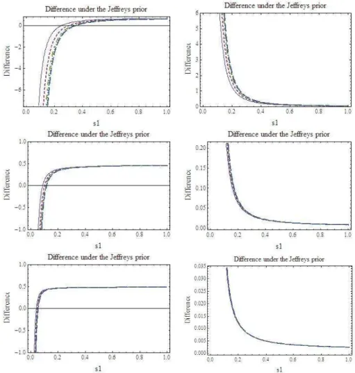
In Figure 2.1, we plotn2₍_g

1−g2) as a function ofs1withs2= 1, forn= 10,20,50,100,1000 and m = 2,5,10 respectively. The plots on the left is for the Bayesian predictive densities under the Jeffreys prior, and the plots on the right are for those under the improper prior with

α = 0.9. These plots numerically show that the asymptotic results in Theorem 2 and 3 are also valid for finite sample size with nas small as 10: The Jeffreys prior are not second order KL REML-dominant while the improper prior with α = 0.9 are for all the m(= 2,5,10) and

n(= 10,20,50,100,1000) combinations considered. For the Jeffreys prior, the threshold for the Bayesian predictive distribution to be better than the REML based estimative distribution is between _m1 and _2m1 , which is also consistent with the asymptotic results.

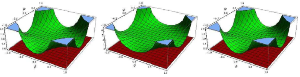
In Figure 2.2, we make two 3-dimensional plots from different angles forn2(g1−g2) withg1 calculated under the improper prior, whenm= 100. Both the left and right panel show clearly that, there is someα∗ _{such that} _when_α_∈_[_α∗_,_{1), the difference will always be positive.}

2.4.3 Simulation Studies

In this section we compare both the Jeffreys prior and the proposed improper prior with the REML estimative density in terms ofEY|θ(D(ϕ,ϕb)−D(ϕ,ϕ˜)) using simulation. The following parts gives the implementation details of the numerical procedure for conducting the simulation experiments, and the simulation results are summarized in the last part.

REML estimator for (s1, s2)

(44)

Figure 2.1: Plots ofn2₍_g

1−g2) against s1 whens2 = 1, forn=10 (thin solid line), 20 (broken line),

50 (broken/dotted line), 100 (dotted line),and 1000 (wider broken line). The plots on the left are for the Bayesian predictive densities under the Jeffreys prior, and those on the right are for those under

the improper prior, withα= 0.9. The three rows from top to bottom correspond tom = 2,5, and 10

(45)

Figure 2.2: Plots ofn2₍_g

1−g2) againsts1 with s2 = 1 when n→ ∞, m= 100 under the improper

prior. All the plots are made fors1∈(0,0.2), α∈(0,1), with views from different angles.

explicitly calculate the REML estimator fors1, s2. The restricted log-likelihood forθ= (s1, s2) is

ℓn(θ) = (1−₂m)nlogs2+1−₂nlog(s2+ms1)−G

2

2 , (2.32)

with

G2 =G2(θ) =YT_{V−1₋V−1X(XTV X)−1XTV−1_}Y

= _s1

2 X

i,j

y_i,j2 ₋_mn(s1 2+ms1)(

X

i,j

yi,j)2− _s₂_(s₂s_+ms1 ₁₎

X

i (X

j

yi,j)2 . (2.33)

For general n andm,

ˆ

s1=

nPn_i₌₁(Pm_j₌₁yi,j)2−(Pni=1

Pm

j=1yi,j)2

m2_n(n₋₁₎ −

mPn_i₌₁Pm_j₌₁y2

i,j−

Pn

i=1(

Pm

j=1yi,j)2

m2_n(m₋₁₎ , (2.34)

and

ˆ

s2 =

mPn_i₌₁Pm_j₌₁y2

i,j−

Pn

i=1(

Pm

j=1yi,j)2

(m−1)mn . (2.35)

It is easy to check that ∂2ℓn(θ)

∂s2 1 ,

∂2_ℓ_n_(θ)

∂s2

(46)

REML estimators goes asymptotically to 0 as ngoes into infinity.

Sampling for (β, s1, s2)

To calculate the predictive density function, we need to generate s1, s2 from the posterior distributions. For both the Jeffreys and improper priors, the marginal posterior is complicated. However, the Metropolis-Hastings algorithm can be used to generate the posterior distributions as follows:

Step 1. Start with arbitrarys0

1, s02 from support of the posterior distribution, i.e. (0,∞). Step 2. At stage n, generate proposal s∗

1, s∗2 from q(s1∗, s∗2|s1, s2). The arbitrary proposal distribution is defined asq(s∗₁, s∗₂_|s1, s2) = _s₁1_s₂ exp{−s

∗

1

s1 −

s∗

2

s2},the product of two exponentials

with meanss1 ands2.

Step 3. Takesn+1₁ =s∗₁, sn+1₂ =s∗₂ with probabilityα= min_{q(s1,s2|s∗1,s∗2)πJ(s∗1,s∗2)f(y|s∗1,s∗2)

q(s∗

1,s∗2|s1,s2)πJ(s1,s2)f(y|s1,s2),1}.

Otherwise, increase n and return toStep 2. This random acceptance is done by generatingu_∼

Uniform (0, 1) and accepting the proposals∗₁, s∗₂ ifu_≤α.

We burn in 1000 out of 2000 simulations (actually 100-500 is enough) to make sure that there is no influence of the initial values for s1 and s2, so only 1000 variates have been used to approximate the posteriors, from which we select one in every ten and make records of 100 pairs of (s∗₁, s∗₂). The convergence is justified by the results of Gelman and Rubin’s convergence diagnostics in the “CODA” package (Output analysis and diagnostics for MCMC simulations) of R language. The procedure is as follows:

1. Run two parallel chains, each with 1000 pairs of (s1, s2) starting from different initial values.

(47)

3. Calculate the “potential scale reduction factor” (see Gelman and Rubin (1992), Brooks and Gelman (1997)) for each parameter (s1 and s2) in the chains, together with upper and lower confidence limits. Approximate convergence is diagnosed, since the upper limits are close to 1, indicating both chains have “forgotten” their initial values, and the output from them is indistinguishable.

We also use the Geweke’s convergence diagnostic to double-check the convergence: first combine the remaining two chains (2_×500 = 1000 draws) to produce one chain, and calculate Z-scores for a test of equality of means (see Geweke (1992)) between the first 10% and last 50% (the CODA default values) of the chain for both parameters. The calculated values do not fall in the extreme tails of a standard normal distribution, providing no evidence against convergence.

MC Method for integration of KL divergence

We evaluateEY|θ[D(ϕ,ϕb)−D(ϕ,ϕ˜)] for fixedθ by the following algorithm. Step 1: Generate Y(l) forl= 1,2, . . . , Lusing the model (2.30) for fixed θ.

Step 2: For each Y(l), compute the REML estimator ˆθ = ( ˆs1,sˆ2) using (2.34) and (2.35), and the corresponding REML predictive density function is given by ˆϕ(z;Y) =ϕ(z;Y,θˆ).

Step 3: Approximate ˜ϕ(z;Y(l)_{) by} 1 n

P

iϕ(z;Y(l), θi), where θi is generated as described in 4.3.2, with Jeffreys and improper priors, respectively.

Step 4: The difference between D(ϕ,ϕˆ) and D(ϕ,ϕ˜) is approximated by quadrature inte-gration method.

Step 5: To calculate the expected KL divergence for fixed θ, we approximate it by 1

L

P

l(D(ϕ,ϕb|Y(l), θ)−D(ϕ,ϕ˜|Y(l), θ)), where the summation is taken over Y(l).

(48)

package of R programming.

Simulation Results

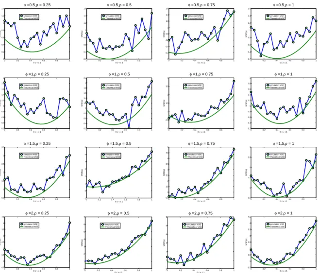
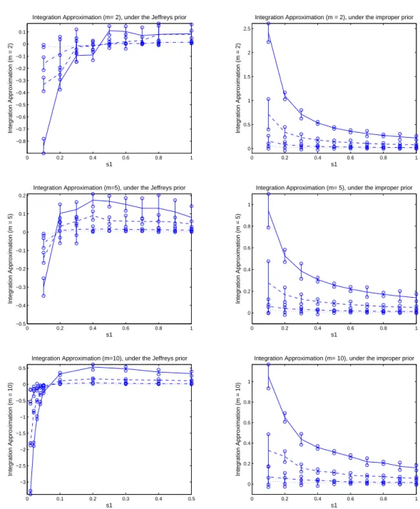
In the simulation studies, we set s2 = 1, β = 0, m = 2,5,10, n = 10,20,50,100, and s1 = 0.1,0.2,0.3,0.4,0.5,0.6,0.7,0.8, and carried out the computation for both the Jeffreys prior and the improper prior with α= 0.75. The results are summarized in Figure 2.3.

The first row of Figure 2.3 describes simulation results form= 2. The left panel shows the results under Jeffreys prior, and the right one under the improper prior withα= 0.75. The left panel indicates that under the Jeffreys prior and when s1 is less than 0.5, the REML plug-in density performs better than the Bayesian predictive density in terms of KL divergence, while the Bayes predictive density performs better than the REML competitor otherwise. The right panel indicates that, under the improper prior the Bayesian predictive density always performs better than the REML estimative density. Both results are consistent with our theoretical findings.

The second row of Figure 2.3 gives simulation results for m = 5. The left panel indicates that when m = 5, the Bayesian predictive density under Jeffreys prior performs better than REML plug-in estimative density when s1

s2 is greater than some value around 0.2, and the

REML competitor performs better otherwise, which is consistent with the asymptotic results in Figure 2.1. The right panel displays simulation results under the improper prior withα= 0.75, which indicates that the Bayesian predictive densities always performs better than the REML estimative density, which are also consistent with the theoretical results.

(49)

0 0.2 0.4 0.6 0.8 1 −0.8 −0.7 −0.6 −0.5 −0.4 −0.3 −0.2 −0.1 0 0.1 s1

Integration Approximation (m = 2)

Integration Approximation (m= 2), under the Jeffreys prior

0 0.2 0.4 0.6 0.8 1

0 0.5 1 1.5 2 2.5 s1

Integration Approximation (m = 2), under the improper prior

0 0.2 0.4 0.6 0.8 1

−0.5 −0.4 −0.3 −0.2 −0.1 0 0.1 0.2 s1

Integration Approximation (m=5), under the Jeffreys prior

0 0.2 0.4 0.6 0.8 1

0 0.2 0.4 0.6 0.8 1 s1

Integration Approximation (m= 5), under the improper prior

0 0.1 0.2 0.3 0.4 0.5

−3 −2.5 −2 −1.5 −1 −0.5 0 0.5 s1

Integration Approximation (m=10), under the Jeffreys prior

0 0.2 0.4 0.6 0.8 1

0 0.2 0.4 0.6 0.8 1 s1

Integration Approximation (m= 10), under the improper prior

(50)

2.5 Discussion

In this chapter we used the asymptotic expansion of the KL divergence as the main tool to compare different predictive distributions, and derived some explicit results for one-way random effects models. In particular, we find a class of improper priors which leads to predictive distributions that are asymptotically superior to the REML based estimative distributions. Similar results have the potential to hold for more general mixed effects models, including the spatial linear models commonly used in geostatistics, nevertheless the proof will be explored elsewhere. The asymptotic expressions we derived for KL divergence is quite general, and can be used for other purpose, such as spatial sampling design in the context of spatial linear model. Vidoni (1995) introduced a simple form to express the predictive densities by approximating the sampling distribution of the maximum likelihood estimator with the p∗-formula and then using Laplace approximation to integrate out the parameter, for exponential families and for location models. We could also consider the similar idea when computing the KL divergence by integrating out the parameter. In particular, we can introduce a design criteria that takes into account of the Kullback-Leibler divergence between the true density and the REML plug-in density or the Bayesian predictive density, with respect to the poplug-int or block predictor. To achieve the optimal design, it is reasonable to consider employing the asymptotic approximation to the KL divergence to the second order, which we obtain as equation (2.25). This might give some explicit form for the integration of Kullback-Leibler divergences, and possibly reduces the computation workload.

(51)

(52)

Chapter 3 Applications to regression models with

temporally or spatially correlated errors

3.1 Introduction

We continue to make intensive exploration on another correlation structure: AR(p) process, instead of the linear mixed effect model, by using theoretical methods in Chapter 2. The p -th order autoregressive (AR(p)) model is widely known in time series analysis. It consists of the data _{yt}, satisfying yt = −Ppi=1aiyt−i +ut, t = 1,· · ·, T, where {ut} is a white noise with mean 0 and variance σ2_{. The point estimation of the AR parameters} _a

(53)

They compared different noninformative priors based on the mean squared error or coverage probability. They considered three candidate priors when making frequentist comparison: the uniform prior (which results in MLE estimator of ρ), the Jeffreys prior, and the symmetrized reference prior, which is the reference prior for_|ρ_|<1. According to their simulation results for mean squared error, the symmetrized reference prior seemed generally superior with exception of the explosive case (_|ρ_|>1). On the other aspect, the coverage for the symmetrized reference prior was generally more attractive as well. Therefore they highly recommended symmetrized reference prior as the “default” prior for the AR(1) model.

Tanaka and Komaki (2005) looked at the Bayesian estimation of the spectral density of the AR(2) model and proposed a superharmonic prior as a noninformative prior. They also considered a more general case, the autoregressive moving average (ARMA) model, focusing on the Bayesian estimation of an unknown spectral density in the ARMA model. They first showed that in the i.i.d. cases, the Bayesian spectral densities based on a superharmonic prior asymptotically dominate those based on the Jeffreys prior, using the asymptotic expansion of the risk difference. Then they obtained the asymptotic expansion of the Bayesian spectral density for the ARMA model, which could be written in the differential-geometrical quantities as in the i.i.d. cases. Finally they obtained a similar result in the ARMA model.

(54)

In particular, Basu and Reinsel (1993) considered the spatial processes defined on a regular rectangular grid in two dimensions with sites labeled (i, j), with an associated random variable

Yij defined at each site. Examples of such phenomena include data collected on a regular grid of size m_×n from satellites and from agricultural field trials. They concentrated on the first-order unilateral models of interest, including a special case of the multiplicative (or linear-by-linear) first-order spatial models, which have proved to be of practical use in modeling of two-dimensional spatial lattice data. No previous work has considered the prior for this kind of linear-by-linear spatial model before.

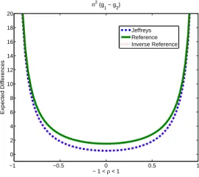
Our work assumes the stationarity, and focuses on both the Bayesian estimation and fre-quentist estimative method for the predictive density of the AR(1) model with unknownσ2, by utilizing the criterion of expected K-L divergence, as proposed in Chapter 2. We point out that the reference prior is superior to the Jeffreys prior and the reference inverse prior, with respect to the second-order asymptotic approximation (see Sections 3.3.3 - 3.3.4). We also consider the noninformative priors and REML estimative density for the model with noise from a spatial multiplicative AR(1) model (see Basu and Reinsel (1993) and Martin (1990)), with fixedσ2 _for simplicity (see Sections 3.4.3 - 3.4.4).

(55)

approach to the AR(1) model, for time series and spatial structure, respectively. We consider three candidate priors: the Jeffreys prior, the reference prior and the inverse reference prior. In an asymptotic sense, all the three priors perform quite well when compared to the REML-plug in density. In particular, we prove that the reference prior dominates the other two priors. In Section 3.3.4 and 3.4.4, we perform the numerical simulation for the AR(1) time series and spatial process, illustrating that the asymptotic results hold,when the sample size is moderately large. In Section 3.5, we make some concluding remarks for our work.

3.2 Review of Noninformative Priors

3.2.1 Background

The use of noninformative priors has an extensive tradition in statistics, starting with Bayes (1763) and Laplace (1812) who used the “uniform” prior

πU(θ) = 1. (3.1)

In developing the Bayesian methodology, use of πU was generally very successful, although there were concerns about its lack of invariance to transformation (because one cannot, for instance, be simultaneously “uniform” inθandη= log(θ)). Also, a number of counterexamples to its use have been encountered, see for example, Mitchell (1967), Monette et al. (1984) and Ye and Berger (1991).

Jeffreys (1961b) sought to overcome the lack of invariance of πU through the development of the now-famous Jeffreys prior

πJ(θ) =

p

(56)

whereI(θ) is the Fisher information matrix with (i, j) entry

I(θ) =₋Eθ[ ∂

2

∂θi∂θjlogf(Y|θ)], (3.3)

where f is the likelihood function of Y given θ, andEθ stands for expectation over X, given

θ. This prior is invariant to reparameterization of the problem, and this method of deriving a noninformative prior seems to correct a number of the counterexamples to use of πU(θ) = 1, especially those arising from nonintegrability of the posterior distribution, πU(θ|data). For instance, for the AR(1) model, with θ= (ρ, σ2_{) where we assume}_|_ρ_|_<_{1 (the stationary case),}

πJ(θ) =

p

I(θ)_∝σ−2(1₋ρ2)−1/2, (3.4)

(see Jeffreys (1961b), Zellner (1971), and Box and Jenkins (1976), for the _|ρ_| < 1 case and Phillips (1991) for the general case). At _|ρ_| = 1, πJ(θ) can be defined by continuity (see Phillips (1991)). In our work we only consider the stationary case.

3.2.2 The Reference Prior Approach

Bernardo (1979) initiated an information-based approach to the development of noninformative priors, called the reference prior approach. A review and discussion of the current status of the approach can be found in Berger and Bernardo (1992).