A geometric view on Pearson’s correlation
coefficient and a generalization of it to
non-linear dependencies
Priyantha Wijayatunga
Department of Statistics, Ume˚a School of Business and Economics,
Ume˚a University, Ume˚a 901 87, Sweden [email protected]
Abstract
Measuring strength or degree of statistical dependence between two ran-dom variables is a common problem in many ran-domains. Pearson’s correlation coefficientρis an accurate measure of linear dependence. We show thatρis a normalized, Euclidean type distance between joint probability distribution of the two random variables and that when their independence is assumed while keeping their marginal distributions. And the normalizing constant is the geometric mean of two maximal distances; each between the joint probability distribution when the full linear dependence is assumed while preserving respective marginal distribution and that when the independence is assumed. Usage of it is restricted to linear dependence because it is based on Euclidean type distances that are generally not metrics and considered full dependence is linear. Therefore, we argue that if a suitable distance metric is used while considering all possible maximal dependences then it can measure any non-linear dependence. But then, one must define all the full dependences. Hellinger distance that is a metric can be used as the dis-tance measure between probability distributions and obtain a generalization ofρfor the discrete case.
Keywords: metric/distance; probability simplex; normalization.
2010 AMS subject classifications: 62H20
doi: 10.23755/rm.v30i1.5
1
Introduction
Measuring association between two random quantities is of interest in many types statistical analyses and applications in various disciplines. Pearson’s product moment correlation coefficient is the standard in statistical textbooks and appli-cations for measuring linear association. And Spearman’s rank correlation coef-ficient is capable of measuring any monotonic dependence between two random variables. For two ordinal variables Cram´er’s V-statistic is widely used whereas Tchuprow’s T-statistic is less-known and therefore less often used (see [14] and references therein). Furthermore, there are many other kinds of dependence mea-sures used in statistical literature, especially in applied statistical analyses. In sta-tistical genetics for evaluation of linkage disequilibrium between genetic markers, authors of [2] use volume tests that are discussed in [10] as a measures of depen-dence between ordinal variables with fixed margins. For massive datasets in [8] it is used mutual information dimension that is defined in terms of information dimension descried in [1].
In [9] it is said that“although it is customary in bivariate data analysis to com-pute a correlation measure of some sort, one number (or index) alone can never fully reveal the nature of dependence; hence a variety of measures are needed”. It is also stated therein that “if (two quantities are) not totally dependent, then it may be helpful to find some quantities that can measure the strength or degree of dependence between them”. In this article we try to develop a measure that can in-dicate ‘the’ degree or strength of association between two discrete variables. Our measure can be seen as a generalization of the Pearson’s correlation coefficientρ
using a suitable distance metric between joint probability distributions, instead of simple Euclidean type distances that are used in ρ (see below). Given the joint probability distribution (jpd) of two discrete variables, say, X and Y, the degree of dependence (also called association) between them is expressed as the normal-ized distance between the jpd of them and that of when the independence of them is assumed. The associated normalizing constant is geometric mean of distances between the latter and all possible jpds where full dependence between X and
corre-sponding to the given dependence. This aspect can make numerical evaluation of the measure algorithmic or computational since sometimes it may not be possible to obtain the full dependences easily. However, here we do not deal with such computational issues but our consideration is on defining a measure following the structure of ρ. For a given dependence (in terms of a jpd) finding efficiently re-lated jpds representing the full dependences that preserve either of the marginal is an open problem.
First we show that, in the simple case of binaryXandY, the ρmeasures the degree of dependence with a certain type of Euclidean distance, but for multi-nary case (and also for continuous variables) a distance in terms another type of Euclidean area is used. But these Euclidean type distances are appropriate for measuring only linear dependences. Since we are interested in measuring any non-linear dependence we propose to use Hellinger distance between joint prob-ability distributions, that is called as Matsusita distance in the discrete (see [6]). The Hellinger distance is a metric and it possesses the so-called linear invariance properties, so it is more suitable for measuring distances between the probability distributions. Therefore, it can be used to measure any type of dependence.
2
Pearson’s correlation coefficient
ρ
For random variablesX andY,the Pearson’s correlation coefficientρ(X, Y) is such that|ρ(X, Y)| ≤ 1. The equality holds if and only if X andY are fully linearly dependent and ρ(X, Y) = 0 if they are linearly independent. And the converse of the latter is not always true unless X and Y are binary. Note that the full dependence is linear in the binary (also called2×2) case where then the
ρ(X, Y)is often calledφ-coefficient.
2.1
2
×
2
case:
φ
-coefficient
LetXandY be two binary variables with a common state space{0,1}where their jpds and marginal probability distributions are written as pxy = p(X =
x, Y = y), px = p(X = x) and qy = p(Y = y) for x, y = 0,1. Let P =
p00 p01
p10 p11
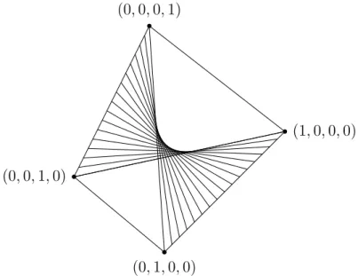
for short. As shown in [12], any such P can be represneted as a point in the probability simplex shown in the Figure 1. The jpd ofX andY under the assumption that they are independent while keeping the marginal distributions fixed isPI =
p0q0 p0q1
p1q0 p1q1
and the set of such probability distributions for all
ofXandY is defined by
φ = p p11−p1q1
p1(1−p1)q1(1−q1)
,
which is a measure of degree of association between X and Y. Now let X
and Y be positively correlated, then there are two jpds under the assumption that the two variables are fully dependent. They are PX =
p0 0
0 p1
and
PY =
q0 0
0 q1
, where PX is when the marginal distribution of X is
pre-served andPY is when the marginal distribution ofY is preserved. Note that each full dependence is obtained from P while preserving respective marginal distri-bution, then the marginal distribution of the other variable should be assumed by it. Therefore in these cases, the full dependence is essentially linear.
For a generalization ofρto measure ‘any’ type of dependence we need to look at its structure and construction. First we consider the case of two binary vari-ables by examining theφ-coefficient. LetDPI,P bep11−p1q1 that is the(2,2)th
component Euclidean distance between the two probability distributions PI and
P. It is a measure of how far the dependence (under P) from the independence (underPI) when marginals ofXandY are fixed. Note that in the2×2case it is sufficient to consider a single component difference (between the two probability matrices) since all the components have same absolute difference. Similarly, we have DPI,PX = p1(1− q1) and DPI,PY = q1(1− p1). Since PX and PY are
the two full dependences that we can obtain from P while preserving respective marginal in each case, we have that DPI,P ≤ DPI,PX and DPI,P ≤ DPI,PY.In
factDPI,P =p11−p1q1 =p1(p11/p1−q1)≤p1(1−q1) =DPI,PX sincep1 ≥p11
and similarly the other inequality. It is easy to see that the denominator of the
φ-coefficient is the geometric mean ofDPI,PX andDPI,PY (the two maximal
dis-tances) and the numerator is DPI,P. Therefore, the φ-coefficient can be thought
of as the normalized distance betweenP andPI where the normalizing constant
is the geometric mean of the two maximal distances. Hence theφ-coefficient is1 if and only ifP =PX = PY (full dependence) and it is0if and only ifPI =P
(independence).
2.2
n
×
m
case
LetX andY be two multinary random variables where their state spaces are {0,1, .., n−1} and {0,1, .., m−1} respectively for n, m > 2. For any given jpd ofX andY, P = (p00, ..., p0(m−1);p10, ..., p1(m−1);...;p(n−1)1, ..., p(n−1)(m−1))
where pij = p(X = i, Y = j) fori = 0, .., n−1 andj = 1, ...m−1, we
de-fine the probability simplex, ∆ = {P = (pij)n×m :
P
(0,1,0,0)
(1,0,0,0)
(0,0,1,0)
(0,0,0,1)
Figure 1: Probability simplex for binary X and Y where their jpd P = (p00, p10, p01, p11)is a point in it. Any jpd on surface shown by lines represents
independence ofXandY.
0,1, .., n − 1;j = 0,1, ..., m − 1} similar to the case of two binary random variables. But here visualization of it is more difficult. Recall that ρ(X, Y) =
cov(X, Y)/pvar(X)V ar(Y), where
cov(X, Y) = X
x,y
xyp(x, y)−X
x
xp(x)X
y
yp(y)
and
var(X) = X
x
x2p(x)− {X
x
xp(x)}2.
In the following we try to visualize theρand its structure for understanding how it measures the dependence.
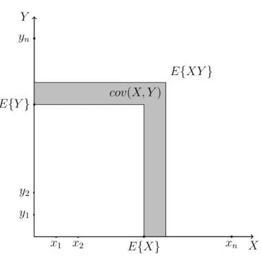
Let us take the case wheren = m, thus allowing us to have perfect (one-to-one) dependence betweenX andY,linear or non-linear. It can be seen that when
X and Y are assigned to two perpendicular axes, cov(X, Y) is area difference between two rectangular Euclidean areas, that is shown as the dark area in the Figure 2. The first area (i.e.,P
x,yxyp(x, y)) is the weighted average area created
X Y
x1 x2 xn
y1
y2
yn
E{XY}
E{X}
E{Y} cov(X, Y)
Figure 2: Covariance ofX andY is the weighted averaged Euclidean area differ-ence.
dependence betweenX andY. And the second area (i.e.,P
xxp(x)×
P
yyp(y))
is the area created by the side lengths that are the weighted average of values of
X (i.e., E{X}) and that ofY (i.e., E{Y}) where the weights are the respective marginal probabilities. Since the lengths or valuesE{X}andE{Y}are also on same axes as X and Y are, respectively, we can see the difference of the two areas. Note that it can be seen that the second area (i.e.,P
x,yxyp(x)p(y)) is also
calculated in the similar way as the first, but assuming the independence ofXand
Y, i.e., it is the weighted average area created by the values ofXandY, where for each component area that is being weighted is with side lengthsX =xandY =y
and the weight associated with it is the respective joint probability ofX = xand
Y =yassuming independencep(X = x, Y =y) = p(X =x)p(Y = y). So the second area represents the scenario of the independence of X andY. Therefore one can view that the two areas refer to those when a dependence betweenXand
Y is assumed and when their independence is assumed while keeping the marginal distributions fixed, thereforecov(X, Y)is a ‘distance’ in terms of a Euclidean area difference between dependence and independence of the two variables.
preserved. Assuming one variable by the other is ‘a way’ to consider a case of full dependence between the two variables. Then we are assuming the marginal ofY
by that ofX. This assumption is easily seen when both variables have same sizes in their state spaces but it is hard to see when they are different. So theE{X2}is
indicated by the weighted average area that we obtain whenY isXwhere weight for each component area x2 is p(x, y) = p(x), i.e., when the marginal of X is preserved. This is a sensible area under full dependence. AndE{X}2is indicated
by the area when the respective weight isp(x)p(y) =p(x)2 wherex=y. This is
a hypothetical case where it is taken as ifY wereX, yet their joint probability is taken as if they were independent. So,var(X)is deviation of the full dependence from independence ifY wereX. And the same interpretation applies forvar(Y). Thus, ρ(X, Y)is the normalized area difference referring to cov(X, Y)with the normalizing constant being the geometric mean of the two maximal area differ-ences referring tocov(X, Y)where they are such that, one is whenY is assumed to beX(i.e.,var(X)) and the other is whenXis assumed to beY (i.e.,var(Y)). That is, the normalizing constant is obtained by assuming the full dependence be-tweenXandY.However the full dependence quantified in this way is appropriate only for doing so for linear dependences. Since there are two such cases of full linear dependence the geometric mean of these two maximal area differences is taken. Note that the above interpretation is valid for the case of X and Y have continuous state spaces.
One thing that we need to show is that cov(X, Y) is maximal (or minimal) when X and Y are strictly monotonically related, for example, linearly related positively (negatively), among all cases of full ono-to-one dependencies between
X and Y for fixed maginals of X and Y. This indicates that ρ is not able to identify non-monotonic relations since their covariance values can not be ordered. To see that cov(X, Y)is maximal whenY is strictly increasing withX, letX = {a1 < ... < an} be the state space ofX andY = {b1 < ... < bn}be that ofY.
Then considering inequalities(ai−aj)(bi−bj)>0fori, j = 1, ..., n(i.e., we have
aibi+ajbj > aibj +ajbi) it can be shown thatPiaibi >Pi,j:j=f(i)aibj wheref
is any one-to-one function fromX toY such thatf(i)6=ifor at least two distinct values ofi(i.e.,fis not a strictly increasing function ofi). Now if the marginals of
X and that ofY are(p1, ..., pn)and(q1, ..., qn), wherepi =qi for alli = 1, ..., n
when Y is monotonically increasing with X and otherwise pi = qj for some
appropriatei 6=j fori, j = 1, ...., n, thenP
iaibipi >
P
i,j:j=f(i)aibjpi meaning
that E{XYM} ≥ E{XY} where YM is Y when it is strictly increasing with
X. This implies that cov(X, YM) ≥ cov(X, Y)for fixed marginals ofX andY.
Therefore, for discreteXandY,ρ(X, Y)is maximal whenY is strictly increasing in X, among all one-to-one relationships between them. So, if this is the case
3
Some other popular measures of dependence
There are a few popular measures of dependence that have similar structure in their definition. We review them briefly by giving some interpretations that support our definition of dependence measure.
3.1
Spearman’s rank correlation coefficient
ρ
sIn many statistical analyses, especially for non-normal data a popular measure of dependence between two random variables, say, X andY, is the Spearman’s rank correlation coefficient.
ρs = 1− 6
Pn
i=1d 2 i
n(n2 −1)
where di = x(i)−y(i) andx(i) is the ith smallest value in the data sample ofX
and similarly for y(i). It is obvious that ρs = 1if and only if two components
of data pair (xi, yi) has the same ranking, for all data pairs since then di = 0
for alli. And one can see that for a perfect negative dependencePn
i=1d 2
i should
be its maximal value that is n(n2 −1)/3 in order to get ρs
X,Y = −1. Therefore
the normalizing constant is taken as n(n2 −1)/6but due to the structure of the
definition of the coefficient it is applied to the term Pn
i=1d 2
i. Therefore the ρs
is an accurate measure any monotonic dependence between the two variables. However, when the two variables are not having a strictly monotonic relationship the measure can not give a correct picture of the dependence.
3.2
Information theoretic measures
Another popular measure of dependence, especially in machine learning lit-erature and applied statistics is so-called mutual information (see, for example, [11]). For discrete random variablesXandY, it is defined as
I(X, Y) = X
x,y
p(x, y)log p(x, y) p(x)p(y)
and furthermore, conditional mutual information betweenXandY given another variableZ is defined as
CI(X, Y, Z) = X
x,y,z
p(x, y, z)log p(x, y|z)
rather divergance, [13]. It is easy to see that I(X, Y) is the KL divergence be-tween the joint probability distribution ofX andY, and that when independence is assumed, therefore it measures the dependence in terms of ‘departure’ from independence. In fact,I(X, Y)is the weighted average of Euclidean distance be-tween logarithmic of the joint probabilityp(x, y)and that when independence is assumed, where weights are the respective joint probabilities. That is, it is the expectation, under the joint probability, of the difference between the logarithmic of the joint probabilityp(x, y)and that when independence is assumed. Note that though 0 ≤ I(., .) ≤ 1, there is no normalization (with respect to any maximal dependence) is involved.
Though these information measures are used to identify respective depen-dences they are not metrics since KL-divergance is not a true distance (metric), therefore they can not be used to measure the degree of dependence between variables. For example, as shown in [7] let p(x, y) and q(x, y) define two de-pendencies between X and Y where p(x, y) =
3/8 1/8 1/8 3/8
and q(x, y) =
1/2 0 1/8 3/8
. Obviously probability distributionq shows a higher dependency than that ofp but its mutual information is lower than that ofp, (M Ip(X, Y) >
M Iq(X, Y)). Note that q is obtained from p without preserving the marginal
distributions of X and Y. Now let r(u, v)and s(u, v) define two dependencies between random variables U and V where r(u, v) =
0 1/7 1/7 1/7 1/7 1/7 1/7 1/7 0
and
s(u, v) =
0 0 2/7 1/7 2/7 0 1/7 1/7 0
. Then we have that M Ir(U, V) < M Is(U, V).
Note thatsshows a higher dependency than that ofrand it is obtained fromrby preserving the marginal distributions ofU andV. Furthermore, all zeros inrare also ins. If this is the case then higher dependency implies higher mutual infor-mation. So mutual information is restricted measure of degree of dependence.
3.3
Chi squared test statistic
χ
2We can see that well-known Chi squared test statisticχ2that is used for testing independence of two discrete random variables uses a certain dependence measure in it for performing the test. LetXandY take valuesi= 1, ..., αandj = 1, ..., β, respectively and let us write the joint probability of X = i and Y = j as pij,
marginal probability ofX = iaspi.and that of Y = iasp.j. So, the conditional
Then,
χ2 =X
i,j
n(pij −pi.p.j)
2
pi.p.j
=nn X
i,j
p2ij pi.p.j
−1
o
=nn X
i,j
pij
pij −pi.p.j
pi.p.j
o
=nn X
i,j
pij
pi|j−pi.
pi.
o
=nn X
i,j
pij
pj|i−p.j
p.j
o
=nE{A}
whereA is a random variable taking the value pi|j−pi.
pi. =
pj|i−p.j
p.j with probability
pij,fori= 1, ..., αandj = 1, ..., β, andEdenotes the expectation. That is,χ2is
n-multiple of the expectation of a random variable whose(i, j)th value is a
‘nor-malized’ distance between the probability valuepi|j andpi.where the normalizing
constant ispi., for alli, j, and vice versa. Note that pi|j−pi.
pi. may be referred to as
the ‘degree’ of dependence between the two events X = i andY = j. In fact, it is the certainty factor for the case pi|j < pi., as described in [4] for measuring
the dependency between the two events and it is a symmetric measure. However, here it is used without the condition. So,E{A}is the expectation of a degree of dependence between the events X = xandY =yfor allx, y.Therefore,E{A} can be thought of as measure of degree of dependence betweenX andY.And the termninχ2makes it a statistic. That is, a statistic for testing dependence between
two variables can be seen as a product of two factors; one is a quantity related the degree of dependence between two variables and the other is that of total number of data cases that are used to estimate the probabilities related to them (i.e., sample information).
3.4
Test of two proportions
Sometimes one may be interested in testing equality of two proportions to see if given two variables are independent, for example, when the outcome (Y) of interest is binary, such as voting, denoted byY = 1 (or not, denoted byY = 0), for a political candidate in an election for two groups/populations (X) such as men, denoted byX = 1,and women, denoted byX = 0. Then one can test if two proportions are equal, i.e.,p(Y = 1|X = 1) =p(Y = 1|X = 0)(let us write it as
p1 =q1) by theZ statistics
Z = p 1
1/a+ 1/b
p1−q1
p
p(1−p)
where a and b are the sizes of the two samples of Y whenX = 1and X = 0, respectively, and p = p(Y = 1). Now we can interpret that the factor √p1−q1
p(1−p)
(p1−q1)in it, where the term
p
p(1−p)should be taken as the normalizing con-stant. Note that the latter is constructed assuming full dependence between the two variables where, then their joint probability distribution isP =
1−p 0 0 p
or similar. Instead of just usingpwhich is the pooled proportion, the geometric mean of p and(1−p)should be used as the normalizing constant. This is necessary to yield the same test statistic value for testing the same hypothesis with com-plementary probabilities i.e., p(Y = 0|X = 1) andp(Y = 0|X = 0). And the term √ 1
1/a+1/b which is a function of sample sizes (sample information) makesZ
a statistics. So, similar to χ2 statistic, Z has a measure of degree of dependence
between the two variables in it, in addition to information on the sample sizes.
4
Axioms of an ideal measure of dependence
Before we define our measure of strength/degree of dependence (or rather a generalization of ρ) it is appropriate to mention axioms that an ideal measure should possess as shown in [3]. However, it is hard to find dependence measures satisfying all these axioms. Our generalization ofρseems to have a bigger poten-tial in satisfying them, but we omit the discussion here. Following are the axioms;
1. It is well-defined for both continuous and discrete case
2. It is normalized such that its value0implies the independence and value1 implies the full dependence (one variable is a deterministic function of the other), where all intermediate degrees of dependencies lie between0and1 3. It is equal or has a simple relationship with the Pearson’s correlation
coeffi-cient in the case of a bivariate normal distribution
4. It is a metric, i.e., it is a true measure of distance (between the independence and dependence of interest) not just a divergence
5. It is invariant under continuous and strictly increasing transformations. These axioms are straightforward and require no further explanation.
able to define the corresponding all possible full dependences, since the measure should be a ratio between a distance from independence to the given dependence and geometric average of distances from independence to the full dependences.
5
Defining a measure of degree of dependence
As we have seen earlier, in the two binary variables(2×2)case where only the linear dependence exists the dependence can be measured by using a single component Euclidean distance between joint probability distributions. However, in the case of two multinary variables (n×n, where n > 2) we can have many types of dependences, and therefore distances among probability distributions can not be defined through only a single component or a weighted average area dif-ference, that are Euclidean type distances and capable of measuring only linear dependences. Therefore we need to use some other suitable distance to measure any non-linear dependences. In the following we discuss a possible distance that is a true metric.
5.1
A metric distance between two probability distributions
We propose to use Hellinger distance between probability distributions (also called Matsushita distance for the discrete case) which is a metric in the proba-bility simplex for our task of measuring dependence. Recall that our dependence measure should be the normalized distance between the given joint probability distribution of the two variables and that when their independence is assumed while preserving the marginals, where the normalizing constant is obtained by considering similar distances related to the all possible maximal dependences but preserving only one of the marginals at each time. LetΦ andΨbe two discrete distribution functions (φ and ψ are probability distributions or mass functions) then the Hellinger distance betweenΦandΨis defined as
M(Φ,Ψ) =
1 2
X
x
p
φ(x)−pψ(x)
21/2
In addition to satisfying properties of a metricM(., .)also satisfies the following properties: (1) 0 ≤ M(Φ,Ψ) ≤ 1, (2)M(Φ(T),Ψ(T)) = M(Φ(T +a),Ψ(T +
a)) for any constant a, and (3) M(Φ(T),Ψ(T)) = M(Φ(cT),Ψ(cT)) for any constantc6= 0where the last two are called thelinear invarianceproperties of the probability metric. Note that M(., .)2
is not a metric.
distribution to a distribution that represent independence is not useful but those with fixed marginals, each at a time. For a given distribution function, say,Φlet us find the maximally Hellinger-distanced distribution functionΨ. The following proposition shows how to find it.
Proposition 5.1. For positive probability distributionφmaximally Hellinger-distanced probability distributionψ is given by
ψ(t) =
(
1, ift = argminuφ(u) 0, otherwise.
and then,M(Φ,Ψ) =n1−pmin{φ(t) :t ∈ T }o1/2 <1.
Proof. Let|T | =n,φ(ti) = φi andψ(ti) = ψi fori = 1, ..., n. Let re-index
allφi’s such thatφ(1) ≥ φ(2) ≥ .... ≥ φ(n) and possibly some of theψi’s can be
zeros. M(Φ,Ψ)is maximal whenP
t∈T p
φ(t)ψ(t)is minimal.
n
X
i=1
p
φiψi = (
p
ψ1+...+
p
ψn)
q
φ(n)
+(pψ1+...+
p
ψn−1)(
q
φ(n−1)−
q
φ(n))
...+pψ1(
q
φ(1)−
q
φ(2))≥
q
φ(n)
That is, Pn
i=1
√
φiψi is minimal whenψ1 = ... =ψn−1 = 0 andψn = 1. So we
obtain the maximally Hellinger-distanced distribution function Ψ and therefore
M(Φ,Ψ).2
But then T is deterministic variable with respect to Ψ! This theorem says that for any given probability distribution, bivariate discrete in our case, the maxi-mally Hellinger-distanced probability distribution is represented by a vertex of the probability simplex. All its component are zeros except for one place that has 1 that is corresponding to the smallest probability value of the reference probability distribution. This is a degenerate case as far as dependence of the two variables are concerned since it represents that both variables are deterministic and hav-ing full dependence. Therefore, such a full dependence can not be used for the normalization since it does not generally preserve the marginals.
full dependence should be preserving either of marginals. This rule is to follow the correlation coefficient definition. Therefore, an essential step is to find the two types of probability distributions PX (jpd(s) representing full dependence when marginal of X is fixed) andPY (jpd(s) representing full dependence when
marginal ofY is fixed) in order to find the normalizing constant. As you will see in some cases there may be multiple candidates for each of them. Therefore we have the following definition. Note that there are some instances such as in [3] and [5] where Hellinger distance between the jpd and that of when independence is assumed is used for measuring the dependence, but in such work no normaliza-tion is done. However, the above proposinormaliza-tion implies that distance between any non-deterministic jpd representing independence and that representing a full de-pendence can be strictly less than 1for two discrete random variables, therefore normalization is necessary if one wants to have a measure that shows strength of dependence.
Definition 5.1. When M is a metric in the probability simplex of two discrete random variables X andY, M-based measure of degree of dependence between
X andY represented by their joint distribution functionP is defined as
ρM(X, Y) = M(P
I, P)
Q
PX∈PX max
Q
PY∈PY max
M(PI, PX)M(PI, PY) 1/|PmaxY +PmaxX |
wherePI is the joint distribution function ofXandY when their independence is
assumed, PX
max denotes the set of all joint distribution functions, each
represent-ing a maximal dependence while preservrepresent-ing the marginal distribution of X and similarly forPY
max,|A|is the cardinality of the setA, andM(P, Q)is the distance
metric between two probability distributionsP andQ.
Note that the denominator is the geometric mean of the maximal distances be-tween full dependences and the independence. And we use Hellinger distance as the distance measure. SinceρM is defined following the structure of the Pearson’s correlation coefficient it can be regarded as a generalization of it for the case of discrete variables.
For linear relationships measuring the dependence is relatively easy since both
PX andPY represent perfect linear dependence. This is when they have all their
there are no pre-specified PX and PY, therefore multiple candidates may exist
for each of them. We argue that they should be induced from the jpd in a similar way to the case of linear dependence. So we propose following simple rule for obtainingPX andPY.
Definition 5.2. For each x, when there exists a single value y0 such that y0 = argmaxyp(X = x, Y = y), then let pX(X = x, Y = y0) = p(X = x) and
pX(X = x, Y 6= y0) = 0to obtainPX. If there are multiple suchy0 values then
obtain multiplePX, each refering to one of thosey0values, assuming that it is the only value where maxima exists. And similarlyPY is defined.
By this way, we get one or more jpds each representing a maximal dependence that preserves respective marginal.
6
Examples of
n
×
n
case where
n
≥
2
Now we consider some different cases of P and demonstrate how we can calculate our measure and compare its value to those of some trational measures.
Case 1 Suppose a simple case of each row and column of P having a single maximal entry that is common to both its row and column. Then the other entries in the row are summed onto the maximal entry in the row for each row to yield
PX and similarlyPY is obtained. Therefore,PX andPY are on the boundary of ∆, so they are the furtherest probability distributions from PI while preserving
respective marginals. Then the degree of dependence betweenXandY is defined as (since|PX
max|=|PmaxY |= 1)
ρM(X, Y) = M(P
I, P)
p
M(PI, PX)M(PI, PY)
Example 6.1. For binary X and Y with P =
0.3 0.2 0.1 0.4
, φ = 0.4082 and
ρM = 0.2783 (Cramer’sV and Tschuprow’s T are 0.4082). And interchanging off-main diagonal entries but keeping the main diagonal entries as they were, i.e.,
havingP =
0.3 0.1 0.2 0.4
, gives the same results for all measures.
Example 6.2. Let state spaces of X and Y be {1,2,3} and their joint
proba-bility P =
0.05 0.03 0.20 0.30 0.07 0.05 0.04 0.20 0.06
PI =
0.1092 0.084 0.0868 0.1638 0.126 0.1302 0.1170 0.090 0.0930
, PX =
0.00 0.00 0.28 0.42 0.00 0.00 0.00 0.30 0.00
andPY =
0.00 0.00 0.31 0.39 0.00 0.00 0.00 0.30 0.00
. And then ρ = −0.2025 but ρM = 0.4113 (Cramer’s
V and Tschuprow’s T are0.5472). But had that P ==
0.05 0.03 0.20 0.04 0.20 0.05 0.30 0.07 0.06
which is a linear dependence then ρ = −0.5474andρM = 0.4075(Cramer’sV
and Tschuprow’sT are 0.5467). Note the change in the degree of dependence is small since linear dependence is obtained from nonlinear case by just interchang-ing probability values inP.
Case 2 When each row and column ofP has a single maximal entry that may not be common to both its row and column we still can obtain a singlePX and a
singlePY. Therefore, we can apply the above definition.
Example 6.3. When P =
0.30 0.03 0.20 0.05 0.07 0.05 0.04 0.20 0.06
we have ρ = 0.1383 and
ρM = 0.450011. Note that here we have that Cramer’s V and Tschuprow’s T
are0.4257843that are lesser than our measure.
Case 3 When there are more than one maximal entry in a row or a column we have multiple PX’s and multiplePY’s. Note that here we try to obtain a similar situation in the above two cases. That is, each row of PX has only one non-zero
element (it is obtained by summing up all entries in the corresponding row ofP, thereby preserving the marginal probability distribution of X). Assume that we get anumber ofPX’s, say, PX1, ..., PXa and bnumber ofPY, say, PY1, ..., PYb.
Let us consider the following example.
Example 6.4. WhenP =
0.11 0.01 0.01 0.01 0.01 0.01 0.01 0.01 0.01 0.25 0.01 0.10 0.10 0.01 0.01 0.01 0.01 0.01 0.15 0.01 0.01 0.10 0.01 0.01 0.01
then we make two
PX1 =
0.15 0.000 0.000 0.00 0.00 0.00 0.000 0.000 0.00 0.29 0.00 0.230 0.000 0.00 0.00 0.00 0.000 0.000 0.19 0.00 0.00 0.140 0.000 0.00 0.00
and
PX2 =
0.15 0.000 0.000 0.00 0.00 0.00 0.000 0.000 0.00 0.29 0.00 0.000 0.230 0.00 0.00 0.00 0.000 0.000 0.19 0.00 0.00 0.140 0.000 0.00 0.00
.
Therefore we have two maximal distances to these two full dependences. They are
M(PI, PX1) and M(PI, PX2) and similarly we obtain another two full
depen-dences when marginal ofY is preserved. Therefore,
ρM(X, Y) = M(P, P
I) Q2 i=1 Q2 j=1
M(PXi, PI)M(PYj, PI)
1 4
Thenρ = −0.0491and ρM = 0.5731. Note that here we have that Cramer’s V
and Tschuprow’sT are0.6652.
7
Conclusion
We have looked at the structure and the construction of the Pearson’s cor-relation coefficient ρ in order to have a generalization of it for measuring any non-linear dependence between two random variables. We have shown that it is simple do it geometrically for discrete variables. It can be shown thatρis a nor-malized ‘Euclidean’ type distance between the joint probability distribution of the two random variables and that when their independence is assumed in the prob-ability simplex of the two variables where normalizing constant is the geometric mean of two maximal such distances; each between full linear dependence of the two variables and their independence while preserving the marginal distribution of respective variable. So, we have shown that if we consider all possible full dependences and use an appropriate distance such as Hellinger then we can have a genaralization of ρ. But generally it is not easy to find all possible maximal distances, which is an open problem that may need algorithmic or computational solutions. However we have shown some examples after having defined a gener-alization.
References
[1] A. R´enyi, Probability Theory North-Holland Publishing Company and Akad´emiai Kiad´o, Publishing House of the Hungarian Academy of Sciences. Republished Dover USA, 2007.
[2] C. Sabatti, Measuring dependency with volume tests, The American Statis-tician 56 3 (2002), 191-195.DOI: 10.1198/000313002128.
[3] C. W. Granger, E. Maasoumi and J. Racine,A Dependence Metric for Possi-bly Nonlinear Processes, The Journal of Time Series Analysis 25 5 (2004), 649-669.
[4] F. Berzal, I. Blanco, D. Sanchez and M. -A. Vila, Measuring the Accuracy and Interest of Association Rules: A New Framework, Intelligent Data Anal-ysis 6 3 (2002), 221-235.
[5] H. Skaug and D. Tjostheim,Testing for serial independence using measures of distance between densities, P. M. Robinson and M. Rosenblatt (Eds): Athens Conference on Applied Probability and Time Series, Volume II: Time Series Analysis In Memory of E.J. Hannan, Springer Lecture Notes in Statistics 115 (1996), 363-377.
[6] K. Matsusita,Decision rules, based on distance, for problems of fit, two sam-ples, and estimation, Annals of Mathematical Statistics 26 4 (1955), 631-640.
[7] M. Studeny and J. Vejnarova, The Multiinformation Function as a Tool for Measuring Stochastic Dependence, M. I. Jordan (Eds): Learning in Graphi-cal Models, Kluwer Academic Publishers (1998), 261-297.
[8] M. Sugiyama and K. M. Borgwardt,Measuring Statistical Dependence via the Mutual Information Dimension, Proceedings of the Twenty-Third Inter-national Joint Conference on Artificial Intelligence (IJCAI’13) AAAI Press (2013), 1692-1698.
[9] N. Balakrishnan and C. -D. Lai, Continuous Bivariate Distributions, Springer, 2009.
[11] P. Wijayatunga, S. Mase and M. Nakamura, Appraisal of Companies with Bayesian Networks, International Journal of Business Intelligence and Data Mining 1 3 (2006), 326-346.
[12] S. E. Fienberg and J. P. Gilbert,The Geometry of a Two by Two Contingency Table, Journal of the American Statistical Association 65 (1970), 694-701 [13] S. Kullback and R. A. Leibler,On information and sufficiency, The Annals
of Mathematical Statistics 22 1 (1951), 79-86