Network Traffic
Classification and Demand
Prediction
Mikhail Dashevskiy and Zhiyuan Luo
Reliable classification of network traffic and accurate demand prediction can offer substantial benefits to service differentiation, enforcement of security poli-cies and traffic engineering for network operators and service providers. For example, dynamic resource allocation with the support of traffic prediction can efficiently utilise the network resources and support quality of service. One of the key requirements for dynamic resource allocation framework is to predict traffic in the next control time interval based on historical data and online mea-surements of traffic characteristics over appropriate timescales. Predictions with reliability measures allow service providers and network carriers to effectively perform a cost-benefit evaluation of alternative actions and optimise network performance such as delay and information loss. In this chapter, we apply conformal predictions to two important problems of the network resource man-agement. Firstly, we discuss reliable network traffic classification using network traffic flow measurement. Secondly, we consider the problem of time series anal-ysis of network resource demand and investigate how to make predictions and build effective prediction intervals. Experimental results on publicly available datasets are presented to demonstrate benefits of the conformal predictions.
12.1
Introduction
The Internet is a global system of interconnected computer networks that use the standard Internet Protocol (IP) suite to serve billions of users all over the world. Various network applications utilise the Internet or other network hard-ware infrastructure to perform useful functions. Network applications often use a client-server architecture, where the client and server are two computers con-nected to the network. The server is programmed to provide some service to the client. For example, in World Wide Web (WWW) the client computer runs a Web client programme like Firefox or Internet Explorer, and the server runs a Web server program like Apache or Internet Information Server where the shared data would be stored and accessed.
The Internet is based on packet switching technology. The information ex-changed between the computers are divided into small data chucks called packets and are controlled by various protocols. Each packet has a header and payload where the header carries the information that will help the packet get to its destination such as the sender’s IP address. The payload carries the data in the protocols that the Internet uses. Each packet is routed independently and transmission resources such as link bandwidth and buffer space are allocated as needed by packets. The principal goals of packet switching are to optimise utilisation of available link capacity, minimise response times and increase the robustness of communication.
In a typical network, the traffic through the network is heterogeneous and consists of flows from multiple applications and utilities. Typically a stream of packets is generated when a user visits a website or sends an email. A traffic flow is uniquely identified by 4-tuple{source IP address, source port number, destination IP address, destination port number}. Two widely used transport layer protocols are Transmission Control Protocol (TCP) and User Datagram Protocol (UDP). The main differences between TCP and UDP are that TCP is connection oriented and a connection is established before the data can be exchanged. On the other hand, UDP is connectionless.
Many different network applications are running on the Internet. The Inter-net traffic is a huge mixture and there are thousands of different applications generate lots of different traffic. In addition to “traditional” applications (e.g. Email and file transfer), new Internet applications such as multimedia stream-ing, blogs, Internet telephony, games and peer-to-peer (P2P) file sharing become popular [253]. Therefore, there are different packet sending and arrival patterns due to interaction between the sender and the receiver and data transmission behaviour. Many of these applications are unique and have their own require-ments with respect to network parameters such as bandwidth, delay and jitter. Loss-tolerant applications such as video conferencing and interactive games can tolerate some amount of data loss. On the other hand, elastic applications such as Email, file transfer and Web transfer can make use of as much, or as lit-tle bandwidth as happens to be available. Elastic Internet applications have the greatest share in the traffic transported over the Internet today. Traffic classification can be defined as methods of classifying traffic data based on
fea-tures passively observed in the traffic, according to specific classification goals. Quality of Service (QoS) is the ability to provide different priority to different applications, users, or data flows, or to guarantee a certain level of performance to a data flow.
The predictability of network traffic is of significant interest in many do-mains. For example, it can be used to improve the QoS mechanisms as well as congestion and resource control by adapting the network parameters to traffic characteristics. Dynamic resource allocation with the support of traffic predic-tion can efficiently utilise the network resources and support QoS. One of the key requirements for dynamic resource allocation framework is to predict traffic in the next control time interval based on historical data and online measure-ments of traffic characteristics over appropriate timescales. Machine learning algorithms are capable of observing and identifying patterns within the statis-tical variations of a monitored parameter such as resource consumption. They can then make appropriate predictions concerning future resource demands us-ing this past behaviour. There are two main approaches to predictions used in dynamic resource allocation: indirectly predicting traffic behaviour descriptors and directly forecasting resource consumption.
In the indirect traffic prediction approach, it is assumed that there is an underlying stochastic model of the network traffic. Time-series modelling is typically used to build such a model from a given traffic trace. First, one wants to determine the likely values of the parameters associated with the model. Then a set of possible models may be selected, and parameter values are determined for each model. Finally, diagnostic checking is carried out to establish how well the estimated model conforms to the observed data. A wide range of time series models has been developed to represent short-range and long-range dependent behaviour in network traffic. However, it is still an open problem regarding how to fit an appropriate model to the given traffic trace. In addition, long execution times are associated with the model selection process.
The direct traffic prediction approach is more fundamental in nature and more challenging than indirect traffic descriptor prediction. This is because one can easily derive any statistical traffic descriptors from the concrete traffic vol-ume, but not vice versa. Different learning and prediction approaches, including conventional statistical methods and machine learning approaches such as neu-ral networks, have been applied to dynamic resource reservation problems [73]. Despite the reported success of these methods in asynchronous transfer mode and wireless networks, the learning and prediction techniques used can only pro-vide simple predictions, i.e. the algorithms make predictions without saying how reliable these predictions are. The reliability of a method is often determined by measuring general accuracy across independent test sets. For learning and prediction algorithms, if we make no prior assumptions about the probability distribution of the data, other than that it is Identically and Independently Dis-tributed (IID), there is no formal confidence relationship between the accuracy of the prediction made with the test data and the prediction associated with a new and unknown case.
and prediction should ideally be adaptive and provide confidence information. In this chapter, we apply conformal predictions to enhance the learning algorithms for network traffic classification and demand prediction problems. The nov-elty of conformal predictions is that they can learn and predict simultaneously, continually improving their performance as they make each new prediction and ascertain how accurate it is. Conformal predictors not only give predictions, but also provide additional information about reliability with their outputs. Note that in the case of regression the predictions output by such algorithms are intervals where the true value is supposed to lie.
The reminder of this chapter is structured as follows. Section 2 discusses the application of conformal predictions to the problem of network traffic clas-sification. Section 3 considers the application of conformal predictions to the network demand predictions and presents a way of constructing reliable predic-tion intervals (i.e. intervals which include point predicpredic-tions) by using conformal predictors. Section 4 shows experimental results of the conformal prediction on public network traffic datasets. Finally, Section 5 presents conclusions.
12.2
Network Traffic Classification
Network traffic classification is an important problem of network resource man-agement that arises from analysing network trends and network planning and designing. Successful classification of network traffic packets can be used in many applications, such as firewalls, intrusion detection systems, status reports and Quality of Service systems ([204]). Approaches to network traffic classifi-cation vary according to the properties of the packets used. Following [204], the following approaches will be briefly examined and discussed: port-based approach, payload-based approach, host behaviour based approach and flow features-based approach.
12.2.1
Port-based Approach
Port-based approach is the fastest and the simplest method to classify network traffic packets and as such has been extensively used [434]. Many applications, such as WWW and Email, have fixed (or traditionally used) port numbers and, thus, traffic belonging to these applications can be easily identified. However, since there are many applications (such as P2P, Games and Multimedia) that do not have fixed port numbers and instead use the port numbers of other widely used applications (e.g. HTTP/FTP connections), this approach some-times yields poor results (see [103, 253, 346]).
12.2.2
Payload-based Classification
Payload-based classification algorithms look at the packets’ contents to identify the type of traffic [346]. When a set of unique payload signatures is collected by an algorithm, this approach results in high performance for most types of traffic,
such as HTTP, FTP and SMTP. However, payload-based classification methods often fail to correctly identify the type of traffic used by P2P and multimedia applications ([274]) due to the fact that these applications use variable payload signatures.
12.2.3
Host Behaviour-based Method
Algorithms which classify traffic by analysing the profile of a host (i.e. the destinations and ports the host communicates with) to determine the type of the traffic are called host behaviour-based methods [152]. Some newly developed methods (such as BLINC, [198]) rely on capturing host behaviour signatures. An advantage of these methods is that they manage to classify traffic even when it is encrypted. A disadvantage is the fact that host behaviour-based methods require the number of flows specific to a particular type of traffic to reach a certain threshold before they are able to be classified.
12.2.4
Flow Feature-based Method
Flow feature-based methods employ machine learning techniques to find a pat-tern in the packets and thus identify the type of traffic based on various sta-tistical features of the flow of packets. Example flow-level features include flow duration, data volume, number of packets, variance of these metrics etc. The machine learning methods which can be used include Naive Bayes, k-Nearest Neighbours, Neural Networks, logistic regression, clustering algorithms and Sup-port Vector Machines (SVM) ([11, 113, 115, 274, 112, 273, 306, 247]). This chapter considers only this approach to network traffic classification.
12.2.5
Our Approach
Many machine learning algorithms have been successfully applied to the prob-lem of network traffic classification ([274, 281, 439, 426]), but usually these algorithms provide bare predictions, i.e. predictions without any measure of how reliable they are. Algorithms that do provide some measure of reliability with their outputs usually make strong assumptions on the data. Bayesian pre-dictors, for example, require the a priori distribution on the data [136]. It was shown in [260] that if this a priori distribution is wrong, the algorithm provides unreliable confidence numbers (measures of reliability).
This section considers the problem of reliable network traffic classification. The aim is to classify network traffic flows and to provide some measure of how reliable the classification is by applying conformal predictors [86, 85, 84]. Conformal predictors is a machine learning technique of making predictions (classifications) according to how similar the current example is to representa-tives of different classes [134, 411]. In machine learning: given a training set ofn−1 labelled examples z1, ..., zn−1) where each example zi consists of an
object xi and its label yi, zi=(xi, yi), and a new unlabelled example xn, we would like to say something about its labelyn [267]. The objects are elements
of an object spaceXand the labels are elements of a finite label spaceY. For example, in traffic classification, xiare multi-dimensional traffic flow statistics vectors and yi are application groups taking only finite number of values such as {WWW, FTP, EMAIL, P2P}. It is assumed that the example sequence is generated according to an IID unknown probability distributionP inZ∞.
Conformal predictors are based on a Nonconformity Measure, a function which gives some measure of dissimilarity between an example and a set of other examples. The higher the value of this function on an example, the more unlikely it is that this example belongs to the selected group of examples. To exploit this idea, we can assign different labels to the current objectxn, calculate the dissimilarity between this example and other examples with the same label, calculate the dissimilarity between this example and examples with other labels, and then use these values to classify the object. In order to describe conformal predictors more precisely we need to introduce some formal definitions.
For eachn= 1,2, . . .we define function An:Zn−1×Z→R
as the restriction of A to Zn−1×Z. Sequence (An : n∈ N) is called a non-conformity measure. To provide a more intuitive idea of what a nonconformity measure is, we need to use the termbag which was defined in the previous sub-section. Given a nonconformity measure (An) and a bag of examples (z1, . . . , zn)
we can calculate the nonconformity score for each example in the bag:
αi=An((z1, . . . , zi−1, zi+1, . . . , zn), zi). (12.1)
The nonconformity score is a measure of how dissimilar one example is from a group of examples. If, for example, the 1-nearest neighbour algorithm is used as the underlying algorithm (the algorithm used to calculate the nonconformity score) for conformal predictors, the nonconformity score can be calculated as
An((z1, . . . , zn), z) =
mini∈{1,...,n},yi=yd(xi, x) mini∈{1,...,n},yi= yd(xi, x).
This formula represents the idea that we consider an example as noncon-forming if it lies much further from the selected group of examples than from all In this thesis, we compare two reliable predictors which make only weak assumptions on the data. In addition, we provide some guidelines on how to choose between the algorithms in practical applications. other examples outside the selected group.
Unlike the Nearest Neighbours algorithm, the Nearest Centroid (NC) algo-rithm (see [31]) does not require computing the distances between each pair of objects. Instead, it measures the distance between an object and the centroid (i.e. the average) of all objects belonging to the same class. The nonconformity measure can be calculated as follows:
αi=αi(xi, yi) = mind(μyi, xi) y=yid(μy, xi),
whereμyis the centroid of all objects with the labely.
Now, to use the nonconformity scores we must compare the current object (which we are trying to classify) with the examples from the training set. In this way, we can see how the current object fits into the “big picture” of the dataset. Now we introduce the termp-value. The number
#|{j= 1, . . . , n:αj≥αn}| n
is calledp-value of objectzn= (xn, yn). Conformal Predictor receives a signif-icance level (a small positive real number reflecting the confidence we want to achieve; it equals one minus the confidence level) as a parameter, and makes predictions, Basically, conformal Predictor calculates the p-values of the pairs (xn,possible label) and outputs all pairs where the p-value is greater than the significance level. Algorithm 14 outlines the scheme by which conformal predic-tors make predictions.
Algorithm 14Conformal Predictor Algorithm for Classification
Input: Parameters{significance level}
for n= 2,3, . . .{at each step of the algorithm}do
forj= 1, . . . , N umberOf Labels{for each possible label} do
Assignyn=j{let us consider that the current example has labelj} Calculateαi, i= 1, . . . , n{calculate nonconformity scores using (12.1)} Calculate pj = |{i=1,...,nn:αi≥αn}|{calculate p-value corresponding to the current possible label}
Output j as a predicted label of the current example with p-valuepj if and only ifpj>
end for end for
Conformal predictors can output multiple (region) predictions, i.e. sets of possible labels for the new object. The main advantage of conformal predictors is their property of validity in online setting: the asymptotic number of errors, that is, erroneous region predictions, can be controlled by the significance level – the error rate we are ready to tolerate which is predefined by the user [411]. Given an error probability, conformal predictor produces a set of labels that also contains the true label with probability 1−[411]. If we want to choose only one label as the prediction (single prediction), it is reasonable to choose the label corresponding to the highestp-value. In this case, however, we do not have any theoretical guarantee on the performance of the algorithm.
12.3
Network Demand Prediction
The need for a network demand model arises as the importance of access to the Internet increases for the delivery of essential services. The ability to predict bandwidth demand is critical for efficient service provisioning and intelligent
decision making in the face of rapidly growing traffic and changing traffic pat-terns [306, 346].
Accurate estimate for message quantity and size directly imply network re-source requirement for bandwidth, memory and processor (CPU) cycles. For efficient management of resources such network bandwidth, an accurate esti-mate of the bandwidth demand of the traffic flowing through the network is required. The bandwidth demand patterns have to be learned to predict the fu-ture behaviour of the traffic. Because the Internet is based on packet switching technology, the duration of time connected to the Internet greatly depends on the efficiency of the movement of packets between different IP addresses. One way to estimate the demand for network resource is to estimate the number of packets in a specific time period. Since each packet in the Internet carries a certain number of bytes worth of information, network traffic demand could be defined in terms of bytes.
When a traffic flow is transmitted via a network, usually there are several routes which can be used for this purpose. We can consider a network as a graph where the nodes are network clients, such as routers, and the edges are communication links. The problem of routing packets in a network belongs to resource management and is important to the performance of a network. A decision making system which routes packets usually relies on a prediction module to estimate future network demand. Network demand can be typically characterised as the bandwidth measured in bytes or number of packets over a particular source destination pair. The behaviour of the traffic is usually modelled in terms of its past statistical properties. For short term estimate of traffic behaviour the statistical properties are assumed to vary slowly and hence daily, weekly and seasonal cycles are not considered. The demand is often obtained by measuring traffic at regular time periods such as seconds or minutes. Therefore, we deal with data in terms of time series. In the time series model, the forecast is based only on past values and assumes that factors that influence the past, the present and the future traffic demand will continue.
To model and predict network traffic demand a number of algorithms can be used. Currently researchers use traditional statistical methods of prediction for time series, such as Auto-Regressive Moving Average (ARMA) [51], which is a general linear model, or machine learning algorithms, such as Neural Networks [386, 73]. The goal of time series forecasting is to model a complex system as a black-box, predicting its behaviour based on historical data. However, neural network method requires human interaction throughout the prediction process (see [298]) and for this reason the approach is not considered in this chapter.
Note that the fact that network traffic demand exhibits long-range depen-dence means that linear models cannot predict it well. It has also been noted that network traffic demand is self-similar ([236]), i.e. the traffic behaves in a similar manner regardless of the time scale. This statement, however, has to be adapted so that it takes into account trends in the traffic demand, such as daily (e.g. at 3am the demand is lower than at noon) or yearly (e.g. towards the end of a year the demand is higher due to its constant increase) trends. The slight difference in the data distribution can be attributed to the daily trend, i.e. when
the time scale is 100 seconds and 1000 observations represent approximately 28 hours of traffic, the daily trend becomes noticeable [82, 83]. This topic is out of the scope of the chapter and for more information, see [82, 88]
12.3.1
Our Approach
An important property of time series prediction which is useful for decision making systems is the reliability of prediction intervals. The problem of apply-ing conformal predictors (a method which could not originally be used for time series) to time series prediction in general and to the network traffic demand prediction problem in particular is considered. For network traffic demand diction, it is particularly important to provide predictions quickly, i.e. for pre-diction algorithms to have low computational complexity, as Quality of Service systems need to react to changes in a network in a timely manner.
We consider conformal predictors for regression and particularly conformal predictors for time series analysis. The challenge of applying conformal predic-tors to the problem of time series analysis lies in the fact that observations of a time series are dependent and, therefore, do not meet the requirement of ex-changeability. The aim of this section is to investigate possible ways of applying conformal predictors to time series data and to study their performance. We will show that conformal predictors provide reliable prediction intervals even though they do not provide a theoretical guarantee on their performance.
Conformal Predictors for Regression
The difference between conformal predictors for classification and conformal predictors for regression begins with the definition of the p-value: since in re-gression there are an infinite number of possible labels, the definition must change slightly. To see how the current example (depending ony, its possible label) fits into the “big picture” of the other examples we compare the non-conformity scores. We again denote objects as xi and labels as yi. Now we introduce the term p-value calculated for the examplezn= (xn, y) as
p(y) = #|{j= 1, . . . , n:αj(y)≥αn(y)}|
n , (12.2)
whereαi(y) is the nonconformity score of objectxiwhen the current observation has labely.
Conformal predictors (as described by Algorithm 15) receive a significance level (a small positive real number equal to the error rate we can tolerate, with the confidence level equal to one minus the significance level) as a parameter. To predict labely for the new examplexn, the Conformal Predictor solves an equation on the variable y so that the p-value of the new example is greater than or equal to the significance level. Usually, the nonconformity measure for regression is designed in such a way that the equation is piecewise linear. For example, we can defineαi =|yi−yˆi|, where ˆyi is the prediction calculated by applying to xi the decision rule found from the dataset without the example
zi[411]. Nonconformity measures were developed for Ridge Regression (and, as
a corollary, Least Squares Regression) in [411].
Algorithm 15Conformal Predictor Algorithm for Regression
Input: significance levelandz1= (x1, y1)
forn= 2,3, . . . do
Get xn
Calculate αi(y), i = 1, . . . , n {calculate nonconformity scores using Equa-tion (12.1)}
Calculatep(y) =#|{i=1,...,n:αin(y)≥αn(y)}| {calculate p-value} Output Γn:={y:p(y)≥}
Get yn
end for
As can be seen above, Algorithm 15 receives feedback on the true label of the objectxn after each prediction is made. This setting “object→prediction
→ true label” is called online mode. When conformal predictors are run in online mode, they are said to be valid as long as they satisfy the assumption of exchangeability of the data. Validity means that the algorithm made a wrong prediction at step n, are independent and have probabilities equal to the pre-defined significance level.
Conformal Predictors for Time Series
A time series is a collection of observations typically sampled at regular intervals. Time series data occur naturally in many application areas such as economics, finance and medicine. A time series model assumes that past patterns will occur in the future. Many network traffic traces are represented as time series. Conformal predictors are designed to be applied to those datasets for which the assumption of exchangeability holds: the elements in the dataset have to be exchangeable, i.e. if we suppose that the elements are the outputs of a probability distribution, then the probability of the occurrence of sequences should not depend on the ordering of the elements in those sequences and, thus, the output of an algorithm applied to such a dataset should not depend on the ordering of the elements. However, in the case of time series, the ordering of the elements of a dataset is essential as the future observations depend only on the current and previous observations.
We extend conformal predictors to the case of time series. To do this, how-ever, we have to either violate or change the restriction on the data required by the algorithm. Thus, we lose the guarantee of validity given by conformal predictors. However, our experiments show that the error rate line is close to a straight line with the slope equal to the significance level (a parameter of the algorithm), which indicates empirical validity.
One way of using conformal predictors for time series data is to assume that there is no long-range dependence between the observations. In this scenario, we
use a parameterT ∈N which specifies how many of the previous observations the current observation can depend on.
Conformal predictors do not fit the framework of time series as they look for the dependence between objects and labels (they predict the new object’s label). To apply them to time series data, we artificially create objects as sets of previous observations.
Suppose we have time series dataa1, a2, a3, . . .whereai∈R∀i. We employ
two methods to generate pairs (object, label) from the time series data. If we want to generate as many pairs as possible and at the same time we do not mind violating the exchangeability requirement, we use the rule
∀i, T + 1≤i≤n:zi= (xi, yi) := ((ai−T, . . . , ai−1), ai),
where n is the length of the time series data. We call these observations de-pendent. If, on the other hand, we want to achieve validity, then we use the rule ∀0≤i≤ n T + 1 −1 :zi= (xi, yi) := (an−i(T+1)−T, . . . , an−i(T+1)−1), an−i(T+1), where [k] is the integer part ofk. These observations are calledindependent.
After transforming the time series data into pairs (object, label) by one of the rules described above, we apply conformal predictors with a nonconformity measure based on some existing algorithm such as Ridge Regression or the Nearest Neighbours algorithm [411]. Now the ordering of the observations is “saved” inside the objects.
To calculate a nonconformity score for objectxn with possible label y, we use prediction ˆy made by an underlying algorithm. We then take function
|y−yˆ| as the nonconformity score, where y is a variable. Note that the only nonconformity score dependent ony is the one for the new exampleαn(y) and that to find the prediction interval it is enough to solve a linear equation ony (see Equation 12.2).
To show an example of how conformal predictors can be applied to time series data, we provide an implementation of conformal predictors based on the 1-Nearest Neighbour algorithm (see Algorithm 16). In this algorithm, r is a possible nonconformity score for the current example and the calculation of ˆyn is provided by the underlying algorithm. To build conformal predictors for time series data using another underlying algorithm, the calculation of ˆyn will be changed accordingly. For example, ˆyn can be a prediction made by an ARMA model [51] or by the Ridge Regression algorithm [411]. In this way, conformal predictors can use the outputs of any time series prediction model to build prediction intervals without constructing objects; in this chapter, we will use this idea to run experiments on conformal predictors for time series analysis.
Algorithm 16Conformal predictors for time series data based on the 1-Nearest Neighbour algorithm
Input: Parametersand y1, y2 x2:=y1 α2(y) := 0 forn= 3,4,5, . . .do xn:=yn−1 ˆ yn:=yarg mini,2≤i≤n−1{|xi−xn|} p:= max{r∈R:#{αi≥r,n2−≤2i≤n−1} ≥}
Output Γn:= [ˆyn−p,yˆn+p] as prediction foryn Get yn
αn(y) :=|yn−yˆn| end for
12.4
Experiments and Results
The effectiveness of conformal predictions can be evaluated on publicly available datasets by using two performance metrics: validity and efficiency [411]. Va-lidity means that the error rate is close to the expected value, which is equal to a predefined constant (one minus the confidence level). Efficiency reflects how useful the predictions output by a conformal predictor are. For a classification problem, a conformal predictor ideally outputs a single prediction at each step, but in practice this does not always happen. we call an algorithm efficient if the average number of output labels is close to one. For time series prediction, we want to make conformal predictors output efficient (narrow) prediction inter-vals which are empirically valid. We conducted our experiments on two tasks: network traffic classification and traffic demand prediction.
12.4.1
Network Traffic Classification Datasets
The Network Traffic Classification Datasets (NTCD) is a collection of thousands of examples of hand-classified TCP flows (we used the datasets after feature selection, performed by other researchers ([274])). The datasets are publicly available athttp://www.cl.cam.ac.uk/research/srg/netos/nprobe/data/papers/ sigmetrics/index.html [272]. Flows are labelled according to the type of traf-fic they represent, for example WWW, EMAIL, FTP or P2P traffic. For each flow, there are 248 features describing simple statistics about packet length and inter-packet timings, and information derived from the TCP protocol such as SYN and ACK count, for details see [275, 243, 244]. There are 11 datasets and Table 12.1 shows the number of TCP flows in each dataset. Eight types of net-work applications are considered: WWW (1), EMAIL (2), FTP (3), ATTACK (4), P2P (5), DATABASE (6), MULTIMEDIA (7) and SERVICES (8).
Feature selection was applied to these datasets in an attempt to optimise the performance of the prediction systems. The Fast Correlation-Based Filter (FCBF) was chosen as the feature selection method, using symmetrical
uncer-Table 12.1: Traffic types by dataset. Dataset 1 2 3 4 5 6 7 8 Total NTCD-1 18211 4146 1511 122 339 238 87 206 24860 NTCD-2 18559 2726 1701 19 94 329 150 220 23798 NTCD-3 18065 1448 2736 41 100 206 136 200 22932 NTCD-4 19641 1429 600 324 114 8 54 113 22283 NTCD-5 18618 1651 928 122 75 0 38 216 21648 NTCD-6 16892 1618 521 134 94 0 42 82 19383 NTCD-7 51982 2771 484 89 116 36 36 293 55807 NTCD-8 51695 2508 551 129 289 43 33 220 55468 NTCD-9 59993 3678 1577 367 249 15 0 337 66216 NTCD-10 54436 6592 930 446 624 1773 0 212 65013 NTCD-12 15597 1799 1513 0 297 295 0 121 19622
Table 12.2: Selected features.
Index Meaning
1 Server Port Number
11 First quartile of bytes in (Ethernet) packet
39 The total number of sack packets seen that carried duplicate SACK (D-SACK) blocks (S→C)
57 The count of all the packets observed arriving out of order. (C → S)
66
If the endpoint requested Time Stamp options as specified in RFC 1323 a “Y” is printed on the respective field. If the option was not requested, an “N” is printed. (C →S)
102
The missed data, calculated as the difference between the TTL stream length and unique bytes sent. If the connection was not complete, this calculation is invalid and an “NA” (Not Available) is printed (S→C).
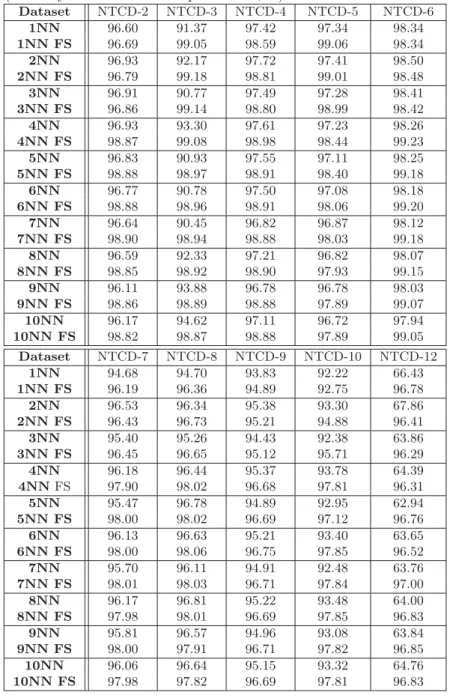
Table 12.3: Performance comparison betweenkNN andkNN with feature selec-tion (accuracy as ratio of correct predicselec-tions, %).
Dataset NTCD-2 NTCD-3 NTCD-4 NTCD-5 NTCD-6 1NN 96.60 91.37 97.42 97.34 98.34 1NN FS 96.69 99.05 98.59 99.06 98.34 2NN 96.93 92.17 97.72 97.41 98.50 2NN FS 96.79 99.18 98.81 99.01 98.48 3NN 96.91 90.77 97.49 97.28 98.41 3NN FS 96.86 99.14 98.80 98.99 98.42 4NN 96.93 93.30 97.61 97.23 98.26 4NN FS 98.87 99.08 98.98 98.44 99.23 5NN 96.83 90.93 97.55 97.11 98.25 5NN FS 98.88 98.97 98.91 98.40 99.18 6NN 96.77 90.78 97.50 97.08 98.18 6NN FS 98.88 98.96 98.91 98.06 99.20 7NN 96.64 90.45 96.82 96.87 98.12 7NN FS 98.90 98.94 98.88 98.03 99.18 8NN 96.59 92.33 97.21 96.82 98.07 8NN FS 98.85 98.92 98.90 97.93 99.15 9NN 96.11 93.88 96.78 96.78 98.03 9NN FS 98.86 98.89 98.88 97.89 99.07 10NN 96.17 94.62 97.11 96.72 97.94 10NN FS 98.82 98.87 98.88 97.89 99.05 Dataset NTCD-7 NTCD-8 NTCD-9 NTCD-10 NTCD-12 1NN 94.68 94.70 93.83 92.22 66.43 1NN FS 96.19 96.36 94.89 92.75 96.78 2NN 96.53 96.34 95.38 93.30 67.86 2NN FS 96.43 96.73 95.21 94.88 96.41 3NN 95.40 95.26 94.43 92.38 63.86 3NN FS 96.45 96.65 95.12 95.71 96.29 4NN 96.18 96.44 95.37 93.78 64.39 4NNFS 97.90 98.02 96.68 97.81 96.31 5NN 95.47 96.78 94.89 92.95 62.94 5NN FS 98.00 98.02 96.69 97.12 96.76 6NN 96.13 96.63 95.21 93.40 63.65 6NN FS 98.00 98.06 96.75 97.85 96.52 7NN 95.70 96.11 94.91 92.48 63.76 7NN FS 98.01 98.03 96.71 97.84 97.00 8NN 96.17 96.81 95.22 93.48 64.00 8NN FS 97.98 98.01 96.69 97.85 96.83 9NN 95.81 96.57 94.96 93.08 63.84 9NN FS 98.00 97.91 96.71 97.82 96.85 10NN 96.06 96.64 95.15 93.32 64.76 10NN FS 97.98 97.82 96.69 97.81 96.83
tainty as the correlation measure [436]. The FCBF method has been shown to be effective in removing both irrelevant and redundant features [437]. This meth-ods is based on the idea that the goodness of a feature can be measured based on its correlation with the class and other good features. The Weka environment ([427]) was used to perform feature selection and the dataset “NTCD-1” was chosen as the training set. Based on the FCBF method, six features out of 248 features were selected and are presented in Table 12.2, whereS→CandC →S mean the flow direction Server to Client and Client to Server, respectively, and “index” represents features in the original datasets. These six features are used in the experiments. Table 12.3 shows the performance of thek-Nearest Neigh-bours algorithm on the datasets with and without feature selection. The table clearly shows the advantages of using feature selection for these datasets.
In the case of multiple predictions, if the true label is a member of the pre-diction set, then the prepre-diction is correct; otherwise, we have a prepre-diction error. As we mentioned early, we are interested validity and efficiency. Validity means that the error rate is close to the expected value, which is equal to a predefined constant (one minus the confidence level). Conformal predictors provide guar-anteed validity (when the assumption of exchangeability holds) [411]. Efficiency reflects how useful the predictions output by a reliable predictor are. Ideally, a reliable predictor outputs a single prediction at each step, but in practice this does not always happen. In this chapter, we call an algorithm efficient if the average number of output labels is close to one.
Figures 12.1 and 12.2 show two examples of experimental results with differ-ent significance level. Figure 12.1 shows that the higher the confidence level is, the lower the total number of errors will be. The graphs of the number of errors over time should be straight lines and the error rates at each point should be approximately equal to the significance level. Figure 12.2 shows that the higher the confidence level is, the higher the number of output labels will be.
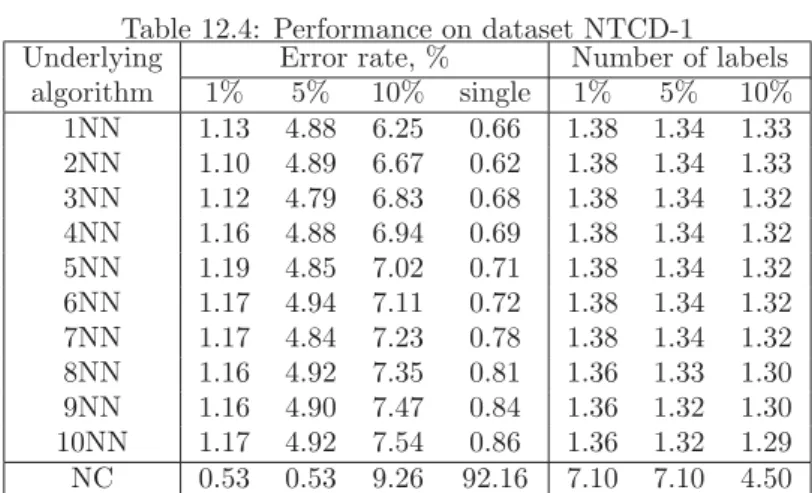
Tables 12.4 and 12.5 show the error rates and average number of labels ob-served when applying conformal predictors to NTCD-1 and NTCD-2 in online setting, respectively. Two underlying algorithms, k-nearest neighbours (NN) and nearest centroid (NC) are used and both region (multiple) predictions and single prediction are considered. The number of nearest neighbours does not significantly affect the performance of the NN algorithm. For both underlying algorithms, the error rates can be controlled by the preset confidence level sub-ject to statistical fluctuations. However, the efficiency of the algorithms changes depending on the dataset. On these two particular datasets, nearest centroid (NC) does not perform as well as the NN algorithm, in particular when single predictions are made.
0 1000 2000 3000 4000 5000 6000 7000 8000 9000 0 100 200 300 400 500 600 examples errors significance level 10% significance level 5% significance level 1%
Figure 12.1: Number of errors for different significance levels (NTCD-1, 3 Near-est Neighbours, multiple predictions)
0 1000 2000 3000 4000 5000 6000 7000 8000 9000 1 1.05 1.1 1.15 1.2 1.25 1.3 1.35 1.4 1.45 1.5 examples
average number of labels
significance level 10% significance level 5% significance level 1%
Figure 12.2: Average number of labels for different significance levels (NTCD-1, 3 Nearest Neighbours, multiple predictions)
Table 12.4: Performance on dataset NTCD-1
Underlying Error rate, % Number of labels
algorithm 1% 5% 10% single 1% 5% 10% 1NN 1.13 4.88 6.25 0.66 1.38 1.34 1.33 2NN 1.10 4.89 6.67 0.62 1.38 1.34 1.33 3NN 1.12 4.79 6.83 0.68 1.38 1.34 1.32 4NN 1.16 4.88 6.94 0.69 1.38 1.34 1.32 5NN 1.19 4.85 7.02 0.71 1.38 1.34 1.32 6NN 1.17 4.94 7.11 0.72 1.38 1.34 1.32 7NN 1.17 4.84 7.23 0.78 1.38 1.34 1.32 8NN 1.16 4.92 7.35 0.81 1.36 1.33 1.30 9NN 1.16 4.90 7.47 0.84 1.36 1.32 1.30 10NN 1.17 4.92 7.54 0.86 1.36 1.32 1.29 NC 0.53 0.53 9.26 92.16 7.10 7.10 4.50
Table 12.5: Performance on dataset NTCD-2
Underlying Error rate, % Number of labels
algorithm 1% 5% 10% single 1% 5% 10% 1NN 0.96 5.18 7.58 0.34 1.90 1.85 1.83 2NN 0.98 5.16 7.87 0.38 1.89 1.85 1.82 3NN 0.96 5.22 8.06 0.38 1.88 1.84 1.81 4NN 1.01 5.22 8.14 0.40 1.88 1.84 1.81 5NN 1.05 5.22 8.19 0.42 1.88 1.84 1.81 6NN 1.03 5.24 8.24 0.42 1.88 1.84 1.81 7NN 1.02 5.23 8.31 0.43 1.88 1.84 1.81 8NN 1.02 5.27 8.38 0.44 1.88 1.84 1.81 9NN 1.02 5.29 8.46 0.45 1.84 1.80 1.77 10NN 1.00 5.23 8.53 0.47 1.66 1.62 1.59 NC 0.50 4.83 7.80 88.94 6.68 6.31 2.32
12.4.2
Network Demand Prediction Datasets
For time series prediction experiments, we used 22 datasets which contained both the number of packets and the number of bytes arriving at (or trans-mitted to and from) a particular facility. The datasets are publicly available athttp://ita.ee.lbl.gov/html/traces.html. Here we briefly describe the datasets, their labelling and some of their properties. Datasets A, B, C and D represent Wide Area Network traffic arriving at the Bellcore Morristown Research and Engineering facility. Datasets E, F, D and H were collected at the same facility and represent only local traffic. Datasets I–P each represent the traffic between Digital Equipment Corporation and the rest of the world during an hour of observation. Similarly, datasets Q, R, S and T each represent the traffic trans-mitted between the Lawrence Berkeley Laboratory and the rest of the world during an hour of observation. Datasets U and V contain information about
Table 12.6: Network traffic demand datasets.
Dataset Name used in literature Measurement No. of Observations
A BC Oct89Ext4 no of bytes 75945 B BC Oct89Ext4 no of packets 75945 C BC Oct89Ext no of bytes 122798 D BC Oct89Ext no of packets 122798 E BC pAug89 no of bytes 3143 F BC pAug89 no of packets 3143 G BC pOct89 no of bytes 1760 H BC pOct89 no of packets 1760 I dec pkt 1 tcp no of bytes 3601 J dec pkt 1 tcp no of packets 3601 K dec pkt 2 tcp no of bytes 3601 L dec pkt 2 tcp no of packets 3601 M dec pkt 3 tcp no of bytes 3600 N dec pkt 3 tcp no of packets 3600 O dec pkt 4 tcp no of bytes 3600 P dec pkt 4 tcp no of packets 3600 Q lbl pkt 4 tcp no of bytes 3600 R lbl pkt 4 tcp no of packets 3600 S lbl pkt 5 tcp no of bytes 3600 T lbl pkt 5 tcp no of packets 3600 U lbl tcp 3 no of bytes 7200 V lbl tcp 3 no of packets 7200
the TCP traffic between the same facility and the rest of the world during two hours of observation.
These datasets have been extensively used in research ([236, 307]). Table 12.6 describes the correspondence between the notation of this chapter and the no-tation used by other researchers, and the values used to create datasets, i.e. the number of bytes or the number of packets transmitted in a network. The original datasets contain the number of bytes in packets and their correspond-ing timestamps. Our datasets contain the aggregated number of bytes and the aggregated number of packets in a network during time intervals of one second. Table 12.6 also shows the number of observations contained in the datasets when the time scale is fixed at one observation per second.
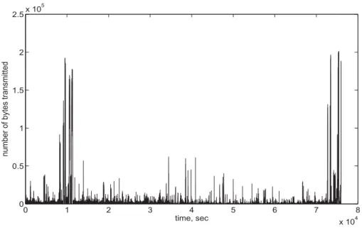
Figure 12.3 shows dataset A (the number of bytes arriving at the Bellcore facility) before pre-processing. Figure 12.4 shows the first 100 entries of the same dataset after pre-processing, which involved subtracting the mean value of the dataset and dividing by the maximum absolute value entry in the dataset. The entries are negative because they are just the first 100 values and in the original dataset they were below the mean value.
Before being used in the experiments, the datasets were pre-processed. For each dataset, we performed the following operations: from each observation, we
0 1 2 3 4 5 6 7 8 x 10⁴ 0 0.5 1 1.5 2 2.5x 10 5 time, sec
number of bytes transmitted
Figure 12.3: Dataset A before pre-processing.
0 10 20 30 40 50 60 70 80 90 100 −0.018 −0.016 −0.014 −0.012 −0.01 −0.008 −0.006 −0.004 −0.002 0 time, sec traffic demand
subtracted the mean value of the dataset and then divided by the largest in absolute value entry. These operations guarantee that the mean value of the datasets is zero and the largest in absolute value entry is 1. If a prediction made for such data exceeds 1 in absolute value, then ether 1 or -1 (whichever is closer to the original prediction) is output as the prediction. During the experiments, the datasets were used with different time scales (i.e. measurement time intervals): 1 second, 2 seconds and 5 seconds for demonstration purposes.
A single long time series can be converted into a set of smaller time series by sliding a window incrementally across the time series. Window length is usually a user defined parameter. Each dataset was divided into sub-datasets of approximately 300 observations. Each of the sub-datasets was used as follows: the first 200 observations were used to build a model and then this model was used to make predictions on the next 100 observations in the online mode, i.e. after each prediction was made, the true value of the observation was passed on to the prediction system. Next, the last 200 observations were used to build another model and this model was used to make predictions on the next 100 observations. Then the process was repeated. This so-called moving window setting divided the experiments into cycles.
There were two purposes to the experiments described in this section. Firstly, we wanted to make sure that conformal predictors output efficient (nar-row) prediction intervals and that they are empirically valid. Empirical validity means that the error rate equals a predefined level, where the error rate is the number of wrong predictions (i.e. predictions which do not contain the real observation of the process) divided by the total number of predictions.
Efficient Prediction with Confidence
To show that conformal predictors are empirically valid and have high efficiency, we experimented with artificial datasets generated by using Autoregressive Mov-ing Average (ARMA) model [51]. ARMA model has two parts, an autoregres-sive (AR) part and a moving average (MA) part. The model is defined as the ARMA(p, q) model wherepis the order of the autoregressive part andq is the order of the moving average part [51]. In our artificially generated datasets, the optimal width of prediction intervals could be calculated and thus we could estimate the efficiency of conformal predictors applied to these datasets [83, 82]. For illustrative purposes, four datasets, X1, X2, X3 and X4 were artificially generated with different parameters p and q. Dataset X1 was generated by an ARMA(2,0) process, dataset X2 by an ARMA(1,2) process, dataset X3 by an ARMA(2,1) process and dataset X4 by an ARMA(0,2) process. All these processes have the variance of the white noise sequence equal to 1, which means that the best possible value for the width of a prediction interval with confidence level of 95% is 3.92, as this is the width of the prediction interval (with the same confidence level) for a normally distributed random variable with variance 1. Of course, the value 3.92 is optimal, but in reality is subject to statistical fluctuations. Therefore, algorithms in the experiments might achieve lower or higher values for the widths of the prediction intervals and still be considered
efficient.
We used eight underlying algorithms before applying conformal predictors to their outputs. The underlying algorithms were the Nearest Neighbours (NN) algorithm with the number of neighbours equal to 1 (with the window size equal to 10) and 3 (with the window size equal to 20), Ridge Regression (RR) with the window size equal to 10 and 20, and the ARMA model with sets of parameters equal to (0,2), (1,1), (2,0) and (2,1).
Table 12.7 shows the widths of the prediction intervals for the last predictions made by conformal predictors based on different underlying algorithms. It can be seen that for the NN algorithm, the widths are much greater than the desired value of 3.92. This is probably due to the fact that the data were generated by linear models and the NN algorithm does not take the linearity of the data into account. Other algorithms, however, are designed to make predictions for data with linear dependence and, with rare exceptions, according to our experimental results, are highly efficient.
Table 12.8 shows the error rates for different algorithms with the significance level of 5%. It can be seen that with few exceptions the error rate of these conformal predictors is close to 5%. It is interesting to note that even though conformal predictors do not provide any guaranteed theoretical validity, the experimental results are still empirically valid.
An interesting property of conformal predictors is that the better the un-derlying algorithm is, the more efficient the conformal predictor based on this algorithm is. Indeed, since the error rate for conformal predictors is guaranteed (in the case where the assumption of exchangeability holds), only the efficiency is important in assessing how successful an underlying algorithm is. Table 12.9 shows the cumulative square errors of different algorithms. It is clear that the algorithms with large errors (such as the NN) have low efficiency whereas the algorithms with small errors (such as the RR) have high efficiency.
To demonstrate that conformal predictors for time series prediction are em-pirically valid, we draw the graph of the cumulative number of errors for different algorithms applied to dataset X1 and the theoretical line which we want the er-ror rates to converge to. Figure 12.5 shows that the cumulative number of erer-rors of different algorithms with significance level of 5% are close to the theoretical value (i.e. the line with the inclination of 0.05).
Figure 12.6 shows the average widths of the prediction intervals for conformal predictors based on different underlying algorithms applied to dataset X1 and the theoretical bound on the width (derived from the properties of the process generating the data). The graph shows that for 4 out of 8 algorithms (namely, RR-WS10, RR-WS20, ARMA(2,0) and ARMA(2,1)), the widths quickly con-verge to the optimal value. The remaining 4 algorithms did not have high performance and thus did not result in efficient conformal predictors.
Table 12.7: Width of the prediction intervals of the last prediction Dataset X1 X2 X3 X4 NN1-WS10 9.22 6.96 7.50 6.71 NN3-WS20 7.66 5.72 6.16 6.93 RR-WS10 4.02 4.01 3.87 4.04 RR-WS20 4.01 3.97 3.90 4.12 ARMA(0,2) 5.20 4.01 4.27 4.02 ARMA(1,1) 5.46 4.95 5.08 4.03 ARMA(2,0) 3.99 4.41 3.92 4.37 ARMA(2,1) 4.00 4.36 3.87 4.03
Table 12.8: Error rates of conformal predictors with significance level of 5%
Dataset X1 X2 X3 X4 NN1-WS10 0.048 0.048 0.050 0.046 NN3-WS20 0.050 0.056 0.050 0.050 RR-WS10 0.045 0.047 0.046 0.046 RR-WS20 0.043 0.044 0.046 0.038 ARMA(0,2) 0.049 0.048 0.052 0.047 ARMA(1,1) 0.045 0.048 0.052 0.045 ARMA(2,0) 0.050 0.050 0.049 0.046 ARMA(2,1) 0.049 0.051 0.047 0.046
Table 12.9: Cumulative square errors of different algorithms
Dataset X1 X2 X3 X4 NN1-WS10 19510 11186 13121 10700 NN3-WS20 14144 7661 8952 11026 RR-WS10 3759 3726 3540 3963 RR-WS20 3769 3629 3568 3938 ARMA(0,2) 6238 3642 4314 3792 ARMA(1,1) 6955 5460 5912 3817 ARMA(2,0) 3702 4434 3541 4505 ARMA(2,1) 3707 4315 3502 3807
0 500 1000 1500 2000 2500 3000 3500 4000 0 20 40 60 80 100 120 140 160 180 observations errors theoretical value algorithm’s errors
Figure 12.5: Cumulative number of errors for conformal predictors with signifi-cance level of 5%, dataset X1
0 500 1000 1500 2000 2500 3000 3500 4000 3 4 5 6 7 8 9 10 11 observations width theoretical bound algorithm’s width
Figure 12.6: Average widths of prediction intervals for conformal predictors, dataset X1
Prediction with Confidence and Guaranteed Performance
The next set of experiments involved building conformal predictors on top of different underlying algorithms. The purpose of the study was to check the experimental validity and efficiency of the algorithm on 22 real network demand traces. We considered 3 underlying algorithms: outputting the mean value of the dataset as the prediction (we call this predictor CONST as it outputs constant values), outputting the last observation as the prediction on the next observation (this predictor is called PREV) and Least Squares Regression (LSR) applied to pairs of two consecutive observations. For each of the datasets we again used time scales of 1, 2 and 5 seconds and made predictions. We built conformal predictors on top of these 3 algorithms and ran them with the significance level equal to 2%, 5% and 10%. We then averaged the error rates and prediction widths over all datasets and time scales.
Table 12.10: Conformal predictors built on top of different algorithms
Algorithm Performance SL-2% SL-5% SL-10%
CONST Error rate 0.019 0.049 0.098
Interval width 1.096 0.773 0.588
PREV Error rate 0.020 0.052 0.102
Interval width 1.143 0.802 0.595
LSR Error rate 0.018 0.051 0.101
Interval width 1.060 0.716 0.524
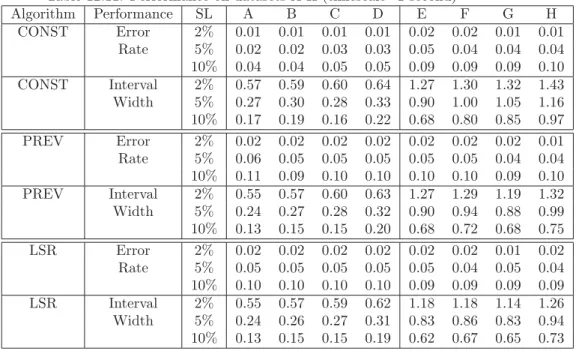
Table 12.10 shows the performance of the three conformal predictors for dif-ferent algorithms and different significance levels (SL), including the average value over all the datasets. From the table it can be seen that the error rates are relatively close to the significance levels. The detailed performance mea-surements on these datasets can be found in Tables 12.11 – 12.19. For example, Tables 12.11, 12.12 and 12.13 show the performance of the different underlying algorithms on the datasets A–H for the timescale of 1, 2 and 5 seconds, respec-tively. Similarly the performance of the different underlying algorithms on the datasets I–P and Q–V can be found in Tables 12.14 – 12.19. It seems that the performance of conformal predictors is not dependent on the measurement used: the number of bytes or the number of packets. The measurement interval can affect the performance of conformal predictors slightly.
Table 12.10 also shows the average widths of the prediction intervals for dif-ferent algorithms. It is worth noting that at the beginning of the prediction process, conformal predictors output the whole range of possible outcomes as the prediction interval and hence the width of the prediction intervals at later steps is smaller than the average width. it can be seen that the width of the prediction interval decreases when the level of the desired error rate increases, which is somewhat intuitive. Indeed, if we want to make fewer mistakes we have
Table 12.11: Performance on datasets A-H (timescale=1 second) Algorithm Performance SL A B C D E F G H CONST Error 2% 0.01 0.01 0.01 0.01 0.02 0.02 0.01 0.01 Rate 5% 0.02 0.02 0.03 0.03 0.05 0.04 0.04 0.04 10% 0.04 0.04 0.05 0.05 0.09 0.09 0.09 0.10 CONST Interval 2% 0.57 0.59 0.60 0.64 1.27 1.30 1.32 1.43 Width 5% 0.27 0.30 0.28 0.33 0.90 1.00 1.05 1.16 10% 0.17 0.19 0.16 0.22 0.68 0.80 0.85 0.97 PREV Error 2% 0.02 0.02 0.02 0.02 0.02 0.02 0.02 0.01 Rate 5% 0.06 0.05 0.05 0.05 0.05 0.05 0.04 0.04 10% 0.11 0.09 0.10 0.10 0.10 0.10 0.09 0.10 PREV Interval 2% 0.55 0.57 0.60 0.63 1.27 1.29 1.19 1.32 Width 5% 0.24 0.27 0.28 0.32 0.90 0.94 0.88 0.99 10% 0.13 0.15 0.15 0.20 0.68 0.72 0.68 0.75 LSR Error 2% 0.02 0.02 0.02 0.02 0.02 0.02 0.01 0.02 Rate 5% 0.05 0.05 0.05 0.05 0.05 0.04 0.05 0.04 10% 0.10 0.10 0.10 0.10 0.09 0.09 0.09 0.09 LSR Interval 2% 0.55 0.57 0.59 0.62 1.18 1.18 1.14 1.26 Width 5% 0.24 0.26 0.27 0.31 0.83 0.86 0.83 0.94 10% 0.13 0.15 0.15 0.19 0.62 0.67 0.65 0.73
to output a wider prediction interval. The table shows that the average pre-diction widths of successful algorithms are smaller than those of less successful algorithms. If we let the algorithm make 10% of predictions incorrectly, then the average prediction width is less than a quarter of the width of the inter-val of possible outcomes, since the observed inter-values are between−1 and 1 after pre-processing.
Table 12.12: Performance on datasets A-H (timescale=2 seconds) Algorithm Performance SL A B C D E F G H CONST Error 2% 0.01 0.01 0.01 0.01 0.01 0.02 0.01 0.01 Rate 5% 0.03 0.03 0.03 0.03 0.04 0.04 0.03 0.05 10% 0.08 0.07 0.06 0.06 0.09 0.08 0.07 0.10 CONST Interval 2% 0.58 0.60 0.60 0.63 1.36 1.25 1.32 1.48 Width 5% 0.28 0.30 0.28 0.32 1.01 0.98 1.05 1.24 10% 0.18 0.20 0.17 0.21 0.79 0.80 0.89 1.09 PREV Error 2% 0.02 0.02 0.02 0.02 0.02 0.02 0.01 0.02 Rate 5% 0.06 0.05 0.06 0.05 0.05 0.04 0.05 0.04 10% 0.11 0.10 0.11 0.10 0.09 0.09 0.10 0.10 PREV Interval 2% 0.55 0.57 0.60 0.62 1.41 1.23 1.17 1.30 Width 5% 0.24 0.26 0.28 0.30 1.07 0.95 0.87 1.03 10% 0.13 0.15 0.15 0.18 0.83 0.73 0.69 0.82 LSR Error 2% 0.02 0.02 0.02 0.02 0.01 0.01 0.02 0.02 Rate 5% 0.05 0.05 0.06 0.05 0.04 0.04 0.04 0.04 10% 0.11 0.10 0.10 0.10 0.08 0.08 0.10 0.10 LSR Interval 2% 0.55 0.57 0.60 0.61 1.29 1.14 1.12 1.27 Width 5% 0.24 0.26 0.27 0.30 0.95 0.88 0.83 0.98 10% 0.13 0.15 0.15 0.18 0.75 0.69 0.65 0.77
Table 12.13: Performance on datasets A-H (timescale=5 seconds)
Algorithm Performance SL A B C D E F G H CONST Error 2% 0.02 0.02 0.02 0.02 0.03 0.03 0.02 0.02 Rate 5% 0.05 0.05 0.05 0.04 0.06 0.07 0.02 0.05 10% 0.11 0.10 0.09 0.09 0.11 0.11 0.05 0.06 CONST Interval 2% 0.59 0.61 0.64 0.70 1.32 1.33 1.77 1.82 Width 5% 0.29 0.31 0.32 0.39 0.98 1.02 1.52 1.69 10% 0.18 0.20 0.19 0.27 0.77 0.79 1.41 1.54 PREV Error 2% 0.02 0.02 0.03 0.02 0.02 0.02 0.00 0.00 Rate 5% 0.06 0.05 0.06 0.05 0.04 0.06 0.04 0.03 10% 0.11 0.10 0.11 0.10 0.12 0.11 0.11 0.11 PREV Interval 2% 0.56 0.58 0.63 0.67 1.40 1.48 1.34 1.38 Width 5% 0.24 0.26 0.30 0.35 1.07 1.12 0.96 1.03 10% 0.13 0.14 0.17 0.21 0.77 0.81 0.69 0.82 LSR Error 2% 0.02 0.02 0.02 0.02 0.03 0.02 0.00 0.00 Rate 5% 0.06 0.05 0.06 0.05 0.04 0.06 0.04 0.03 10% 0.11 0.10 0.11 0.10 0.11 0.11 0.09 0.08 LSR Interval 2% 0.56 0.58 0.62 0.66 1.23 1.27 1.43 1.47 Width 5% 0.24 0.26 0.29 0.34 0.92 0.95 1.01 1.16 10% 0.13 0.14 0.16 0.21 0.68 0.73 0.79 0.90
Table 12.14: Performance on datasets I-P (timescale=1 second) Algorithm Performance SL I J K L M N O P CONST Error 2% 0.02 0.02 0.02 0.02 0.02 0.02 0.02 0.02 Rate 5% 0.05 0.05 0.05 0.05 0.05 0.05 0.05 0.05 10% 0.10 0.10 0.10 0.10 0.10 0.10 0.10 0.10 CONST Interval 2% 1.13 1.02 1.23 1.19 1.04 1.27 1.31 1.29 Width 5% 0.79 0.70 0.92 0.89 0.71 0.96 1.03 1.01 10% 0.60 0.54 0.73 0.70 0.54 0.77 0.82 0.81 PREV Error 2% 0.02 0.02 0.02 0.02 0.02 0.02 0.02 0.02 Rate 5% 0.05 0.05 0.05 0.05 0.05 0.05 0.05 0.04 10% 0.10 0.10 0.09 0.09 0.10 0.10 0.10 0.09 PREV Interval 2% 1.10 0.94 1.25 1.12 1.09 1.27 1.35 1.28 Width 5% 0.77 0.62 0.94 0.79 0.74 0.91 1.04 0.98 10% 0.57 0.44 0.74 0.61 0.55 0.72 0.83 0.78 LSR Error 2% 0.02 0.02 0.02 0.02 0.02 0.01 0.02 0.02 Rate 5% 0.06 0.05 0.05 0.05 0.04 0.06 0.04 0.03 10% 0.10 0.10 0.10 0.10 0.11 0.11 0.09 0.08 LSR Interval 2% 1.06 0.91 1.16 1.07 1.00 1.18 1.25 1.19 Width 5% 0.71 0.58 0.84 0.74 0.66 0.84 0.93 0.88 10% 0.52 0.42 0.65 0.55 0.49 0.65 0.73 0.70
Table 12.15: Performance on datasets I-P (timescale=2 seconds)
Algorithm Performance SL I J K L M N O P CONST Error 2% 0.03 0.02 0.02 0.02 0.02 0.02 0.02 0.02 Rate 5% 0.05 0.05 0.05 0.05 0.05 0.05 0.05 0.05 10% 0.11 0.11 0.10 0.10 0.10 0.10 0.11 0.11 CONST Interval 2% 1.13 0.99 1.20 1.35 1.11 1.46 1.23 1.34 Width 5% 0.79 0.68 0.88 1.04 0.80 1.17 0.91 1.05 10% 0.61 0.50 0.69 0.81 0.62 0.97 0.72 0.85 PREV Error 2% 0.02 0.03 0.02 0.02 0.01 0.01 0.02 0.02 Rate 5% 0.05 0.06 0.06 0.06 0.05 0.04 0.05 0.04 10% 0.11 0.10 0.10 0.11 0.10 0.09 0.10 0.09 PREV Interval 2% 1.11 0.92 1.17 1.28 1.14 1.44 1.27 1.38 Width 5% 0.74 0.57 0.85 0.94 0.79 1.13 0.93 1.03 10% 0.55 0.42 0.68 0.71 0.59 0.89 0.72 0.81 LSR Error 2% 0.02 0.03 0.02 0.02 0.01 0.01 0.02 0.02 Rate 5% 0.05 0.06 0.06 0.05 0.05 0.04 0.04 0.05 10% 0.11 0.10 0.10 0.10 0.10 0.09 0.09 0.09 LSR Interval 2% 1.06 0.89 1.14 1.22 1.05 1.33 1.17 1.27 Width 5% 0.69 0.55 0.80 0.88 0.72 1.01 0.84 0.94 10% 0.52 0.40 0.61 0.67 0.54 0.80 0.65 0.74
Table 12.16: Performance on datasets I-P (timescale=5 seconds) Algorithm Performance SL I J K L M N O P CONST Error 2% 0.03 0.03 0.02 0.01 0.02 0.02 0.04 0.02 Rate 5% 0.06 0.06 0.05 0.04 0.04 0.04 0.07 0.06 10% 0.11 0.11 0.10 0.08 0.08 0.09 0.13 0.10 CONST Interval 2% 1.28 0.94 1.51 1.61 1.27 1.51 1.24 1.44 Width 5% 0.97 0.64 1.15 1.29 0.90 1.23 0.96 1.16 10% 0.74 0.47 0.97 1.00 0.69 0.99 0.78 0.95 PREV Error 2% 0.02 0.03 0.01 0.01 0.01 0.02 0.03 0.02 Rate 5% 0.06 0.06 0.04 0.06 0.03 0.04 0.07 0.06 10% 0.11 0.11 0.11 0.09 0.07 0.08 0.13 0.12 PREV Interval 2% 1.21 0.89 1.46 1.53 1.33 1.58 1.26 1.43 Width 5% 0.85 0.57 1.16 1.19 0.99 1.31 0.87 1.08 10% 0.67 0.44 0.90 0.99 0.75 1.06 0.65 0.80 LSR Error 2% 0.03 0.03 0.02 0.02 0.01 0.02 0.03 0.02 Rate 5% 0.08 0.07 0.04 0.05 0.03 0.03 0.07 0.05 10% 0.12 0.12 0.08 0.10 0.08 0.09 0.11 0.10 LSR Interval 2% 1.15 0.86 1.44 1.50 1.20 1.43 1.15 1.32 Width 5% 0.77 0.54 1.05 1.18 0.86 1.15 0.81 1.00 10% 0.60 0.39 0.82 0.89 0.65 0.90 0.61 0.78
Table 12.17: Performance on datasets Q-V (timescale=1 second)
Algorithm Performance SL Q R S T U V CONST Error 2% 0.02 0.02 0.02 0.02 0.02 0.02 Rate 5% 0.05 0.05 0.05 0.05 0.05 0.05 10% 0.11 0.10 0.10 0.10 0.10 0.10 CONST Interval 2% 0.98 0.92 0.80 0.88 0.81 0.82 Width 5% 0.64 0.59 0.48 0.57 0.48 0.50 10% 0.44 0.42 0.33 0.42 0.32 0.36 PREV Error 2% 0.02 0.02 0.02 0.02 0.02 0.02 Rate 5% 0.05 0.05 0.05 0.05 0.06 0.05 10% 0.09 0.10 0.10 0.09 0.10 0.10 PREV Interval 2% 0.95 0.93 0.80 0.86 0.77 0.79 Width 5% 0.62 0.60 0.48 0.54 0.43 0.47 10% 0.42 0.42 0.32 0.38 0.28 0.33 LSR Error 2% 0.02 0.02 0.02 0.02 0.02 0.02 Rate 5% 0.05 0.05 0.05 0.05 0.05 0.05 10% 0.09 0.10 0.10 0.09 0.10 0.10 LSR Interval 2% 0.93 0.88 0.77 0.83 0.75 0.77 Width 5% 0.57 0.54 0.44 0.51 0.41 0.44 10% 0.39 0.38 0.29 0.35 0.26 0.31
Table 12.18: Performance on datasets Q-V (timescale=2 seconds) Algorithm Performance SL Q R S T U V CONST Error 2% 0.02 0.01 0.02 0.02 0.02 0.02 Rate 5% 0.05 0.05 0.05 0.04 0.06 0.06 10% 0.10 0.09 0.08 0.09 0.11 0.10 CONST Interval 2% 1.19 1.12 0.91 1.02 0.93 0.89 Width 5% 0.79 0.78 0.59 0.72 0.54 0.56 10% 0.54 0.59 0.42 0.57 0.37 0.40 PREV Error 2% 0.02 0.01 0.02 0.02 0.02 0.02 Rate 5% 0.05 0.04 0.05 0.05 0.06 0.05 10% 0.10 0.10 0.10 0.09 0.10 0.09 PREV Interval 2% 1.17 1.16 0.90 0.98 0.88 0.86 Width 5% 0.79 0.83 0.56 0.67 0.51 0.53 10% 0.53 0.60 0.40 0.50 0.33 0.37 LSR Error 2% 0.02 0.01 0.03 0.02 0.02 0.02 Rate 5% 0.05 0.04 0.05 0.05 0.05 0.05 10% 0.10 0.09 0.10 0.09 0.10 0.10 LSR Interval 2% 1.11 1.09 0.85 0.94 0.84 0.83 Width 5% 0.70 0.73 0.52 0.62 0.49 0.50 10% 0.47 0.51 0.36 0.46 0.31 0.35
Table 12.19: Performance on datasets Q-V (timescale=5 seconds)
Algorithm Performance SL Q R S T U V CONST Error 2% 0.02 0.02 0.01 0.01 0.03 0.02 Rate 5% 0.04 0.04 0.04 0.03 0.07 0.06 10% 0.09 0.10 0.08 0.07 0.13 0.12 CONST Interval 2% 1.64 1.22 1.20 1.38 1.03 1.02 Width 5% 1.03 0.84 0.75 0.96 0.63 0.67 10% 0.64 0.62 0.49 0.69 0.46 0.49 PREV Error 2% 0.01 0.02 0.02 0.02 0.03 0.02 Rate 5% 0.04 0.04 0.04 0.04 0.06 0.05 10% 0.09 0.08 0.09 0.09 0.10 0.10 PREV Interval 2% 1.72 1.30 1.09 1.18 1.03 0.95 Width 5% 1.20 0.94 0.73 0.87 0.59 0.62 10% 0.79 0.71 0.48 0.66 0.40 0.46 LSR Error 2% 0.01 0.02 0.01 0.01 0.03 0.02 Rate 5% 0.04 0.04 0.04 0.02 0.06 0.05 10% 0.08 0.08 0.09 0.06 0.11 0.10 LSR Interval 2% 1.59 1.18 1.06 1.20 0.97 0.93 Width 5% 0.93 0.81 0.65 0.80 0.56 0.58 10% 0.66 0.60 0.42 0.59 0.37 0.41
12.5
Conclusions
In this chapter, we described two applications of conformal prediction to net-work resource management problems: netnet-work traffic classification and netnet-work demand prediction. The introduction of prediction algorithms based on con-formal predictors into a network management system can lead to significant improvements in the way a network is managed. For example, the confidence information associated with predictions can be used when evaluating plausible alternative resource allocations over a continuum of timescales. Unlike conven-tional machine learning techniques, the predictions these conformal predictors make are hedged: they incorporate an indicator of their own accuracy and reliability. These accuracy reliability measures allow service provider and net-work carrier to choose appropriate allocation strategies by eliminating unlikely resource demands. Therefore, resource management process can effectively per-form a cost-benefit evaluation of alternative actions.
When analysing network traffic flows through classification, it is important to add some measure of how reliable the classifications are. Most currently used methods either do not provide such a measure of reliability or they make strong assumptions on the data. It has been shown that when these assumptions are violated traditional methods (such as Bayesian methods) become invalid and thus cannot be trusted [260]. On the other hand, conformal predictors make weak assumptions on the data generation process and therefore can be applied more widely.
The second problem considered in the chapter is the prediction of future net-work traffic demand. It is a challenging and important problem and a successful solution leads to great improvements in a network’s performance. Conformal predictors offer a method of providing some measure of confidence placed on top of traffic demand predictions that can be used by higher level decision making systems. The resulted network management system becomes more efficient and has higher performance according to a variety of measures.