Algorithms for sensor validation and multisensor fusion

(1)

!∀#∃

%&∋∋()∋∗+,∋

(2)

ALGORITHMS FOR SENSOR VALIDATION AND MULTISENSOR FUSION

SEAN WELLINGTON

A thesis submitted in partial fulfilment of the requirements of The Nottingham Trent University

and Southampton Institute for the degree of Doctor of Philosophy

(3)

ABSTRACT

Doctor of Philosophy

ALGORITHMS FOR SENSOR VALIDATION AND MULTISENSOR FUSION

by Sean James Wellington

Existing techniques for sensor validation and sensor fusion are often based on analytical

sensor models. Such models can be arbitrarily complex and consequently Gaussian

distributions are often assumed, generally with a detrimental effect on overall system

performance. A holistic approach has therefore been adopted in order to develop two

novel and complementary approaches to sensor validation and fusion based on

empirical data. The first uses the Nadaraya-Watson kernel estimator to provide

competitive sensor fusion. The new algorithm is shown to reliably detect and

compensate for bias errors, spike errors, hardover faults, drift faults and erratic

operation, affecting up to three of the five sensors in the array. The inherent smoothing

action of the kernel estimator provides effective noise cancellation and the fused result

is more accurate than the single ‘best sensor’. A Genetic Algorithm has been used to

optimise the Nadaraya-Watson fuser design.

The second approach uses analytical redundancy to provide the on-line sensor

status output µH∈[0,1], where µH=1 indicates the sensor output is valid and µH=0 when

the sensor has failed. This fuzzy measure is derived from change detection parameters

based on spectral analysis of the sensor output signal. The validation scheme can

reliably detect a wide range of sensor fault conditions. An appropriate context

dependent fusion operator can then be used to perform competitive, cooperative or

complementary sensor fusion, with a status output from the fuser providing a useful

qualitative indication of the status of the sensors used to derive the fused result.

The operation of both schemes is illustrated using data obtained from an array of

thick film metal oxide pH sensor electrodes. An ideal pH electrode will sense only the

activity of hydrogen ions, however the selectivity of the metal oxide device is worse

than the conventional glass electrode. The use of sensor fusion can therefore reduce

measurement uncertainty by combining readings from multiple pH sensors having

complementary responses. The array can be conveniently fabricated by screen printing

(4)

Acknowledgements

I am very grateful to Professor Gurvinder Virk from the Department of Electrical and

Electronic Engineering, University of Portsmouth, for his support; without his

encouragement I probably would not have even started this research project. Thanks are

due also to Professor Graham King of Southampton Institute for his advice and Dr

Jonathan Vincent, also of Southampton Institute, for help with proof reading.

Many colleagues have been generous with their time. I am particularly grateful to Dr

John Atkinson of the Thick Film Unit, Department of Engineering Sciences, University

of Southampton and Dr Russ Sion of C-Cubed Limited. John has provided much useful

information about thick film sensors for chemical analytes.

The thick film sensor data used to illustrate the operation of the various sensor

validation and fusion schemes proposed in this thesis were originated as part of the EU

CRAFT project SpHINX – sensors for measuring pH in inks (BRST-CT98-5521), and

kindly supplied by Dr Russ Sion. Genetic Algorithms were implemented using a

software toolbox written by Dr Jonathan Vincent.

Finally, I am hugely grateful to my family, and in particular my wife, Nikki, for her

boundless patience, love and support.

(5)

List of Figures and Tables

List of Figures

Fig. 1: Fusion of complementary sensor data 13

Fig. 2: Comparison of fusion system architectures 22

Fig. 3: A model of the fusion process 23

Fig. 4: A general taxonomy of the main components of a data fusion system 23

Fig. 5: The JDL Model of the Data Fusion Process 25

Fig. 6: Illustration of evidential intervals 37

Fig. 7: Model-based plant validation and fault diagnosis 47

Fig. 8: Summary of the data and quality parameters specified by the SEVA sensor model

51

Fig. 9: Innovation generation of a general sensor model 57

Fig. 10: The principle of potentiometric measurement 60

Fig. 11: Test results obtained from five thick film pH sensors 64

Fig. 12: Empirical design procedure for N-W fuser 65

Fig. 13: Architecture of the feedforward neural network employed to fuse five pH sensors

66

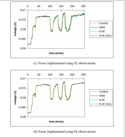
Fig. 14: Effect of altering the number of observations used to realise the fuser 68

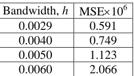
Fig. 15: Effect of altering the bandwidth of the kernel estimator 69

Fig. 16: Genetic algorithm process 73

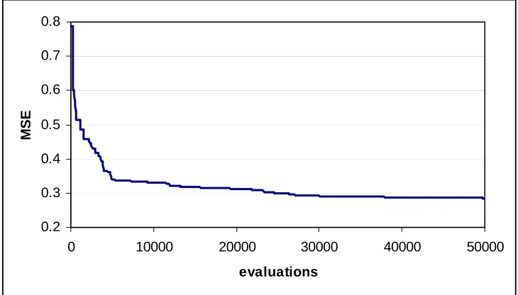
Fig. 17: Typical GA convergence plot 75

Fig. 18: Optimisation of the N-W fuser using a genetic algorithm 76

Fig. 19: Sensor validation using N-W with N=2 81

Fig. 20: Simplified representation of sensor fusion and validation scheme using the N-W estimator

82

Fig. 21: Sensor validation and fusion results using the N-W estimator 86

Fig. 22: Assumed probability density function of a change detection parameter for a healthy sensor

95

(9)

Fig. 24: Comparison of fusion operators 97

Fig. 25: Comparison of ‘context independent variable behaviour’ fusion operators 100

Fig. 26: Deriving change detection parameters by partitioning the frequency spectrum into four separate frequency bands

103

Fig. 27: Comparison of fusion operators for fuzzy change detection parameters 104

Fig. 28: Fuzzy sensor validation using the Fast Fourier Transform 106

Fig. 29: Using a filter-bank to obtain the change detection parameters 108

Fig. 30: Fourier transform of a 16-point Hanning window 109

Fig. 31: Comparison of 64-point Hanning window with 3rd order IIR digital filter 110

Fig. 32: Fuzzy sensor validation using a parallel filterbank 110

Fig. 33: Detecting a sensor stuck fault at t=120 mins. 112

Fig. 34: Fuzzy fusion architecture with sensor validation 114

Fig. 35: Fusion of three thick film pH sensors 115

Fig. 36: Fuzzy sensor validation and fusion with 3 sensors - Sensor 1 spike fault at t=75 mins, Sensor 2 hardover fault at t=150 mins.

116

Fig. 37: Fuzzy sensor validation and fusion with 3 sensors - Sensor 4 erratic from t=100 mins.

117

Fig. 38: Fuzzy sensor validation and fusion with 4 sensors - Sensor 4 erratic from t=100 mins.

118

Fig. 39: Sensor validation and fusion using the N-W kernel estimator 130

Fig. 40: Fuzzy sensor validation 131

(10)

List of Tables

Table 1: JDL Process Model 27

Table 2: Device status values and meanings 51

Table 3: Summary of typical sensor failure modes 52

Table 4: Mean square error of thick film pH sensors 67

Table 5: Effect of altering the number of observations used to realise the fuser 67

Table 6: Effect of altering the bandwidth of the kernel estimator 69

Table 7: Bias and random errors of thick film pH sensors 69

Table 8: Summary of sensor fusion results 69

Table 9: Number of misclassifications for the hypothesis Ho is True if the pH sensor output is greater than –0.075V

71

Table 10: Comparison of decision fusion results obtained using majority voting and a feedforward neural network

71

Table 11: Summary of fuser performance 75

Table 12: Performance of the N-W sensor validation and fusion scheme 84

Table 13: Sensitivity of change detection parameters to sensor faults 103

Table 14: Examples of mathematical tools used for data fusion 122

(11)

1) Introduction

1.1) Background

and

Motivation

In 1997 the UK Foresight Programme highlighted sensors as one of the key areas in

science, engineering and technology that “merit particularly urgent attention by

organisations in the public and private sectors.” Feedback from government, industry

and academia suggested that sensors should be more intelligent, robust, reliable,

integrated and smaller. The report highlighted the need to further develop links between

research into sensor systems and the processing of sensed information, including signal

gathering and processing from multisensor arrays. (Foresight Sensors Action Group,

1997). A separate report by the Defence and Aerospace Foresight Panel Technology

Working Party, also published in 1997, concluded that data fusion and data processing

techniques are vital enabling technologies for a wide range of defence and non-defence

applications (Defence and Aerospace Foresight Panel Technology Working Party,

1997).

Data fusion is not a new concept. A natural ability to fuse sensed information has

evolved in many animal species. Humans for example, routinely combine sight,

hearing, touch, smell and taste information (Murphy, 1996). Data fusion can be used to

calibrate, increase dimensionality, increase statistical significance or provide robustness

in order to cope with sensor uncertainty (Starr and Desforges, 1998). This may be

achieved by:

• Combining readings from several different types of sensor to give more accurate

information;

• Using readings from several independent sensors to make the system less

vulnerable to the failure of a single sensor;

• Combining several readings from the same sensor to reduce the effect of noise (Brooks and Iyengar, 1998).

Present applications of data fusion span a wide range of fields:

• Industrial engineering (Belloir et. al., 2000; Gros, 1997; Karlsson et. al., 1998;

(12)

• Robotics and intelligent vehicles (Agogino et. al., 1995; Bryanston-Cross et. al.,

1999; Dailey et. al., 1996; Durrant-Whyte, 1988; Murphy, 1998);

• Pattern recognition and radar tracking (Belloir and Billat, 2000; Pau and

Trailovic, 2000; Smith, 1998);

• Landmine detection and other military applications (Collins et. al., 2001; Cremer et. al., 1999; Maltese and Lucas, 1998);

• Remote sensing (Leduc et. al., 1999; Petrou and Stassopoulou, 1999);

• Aerospace systems (Doyle and Harris, 1996; Harris et. al., 1998);

• Law enforcement (Hua-Mei Chen and Varshney, 1999; Varshney, 1997a);

• Medicine (Rogova, 1999; Solaiman et. al., 1999; Winquist et. al., 1998).

Data fusion systems have been used extensively for defence applications, in particular

surveillance, target tracking and identification, and strategic decision-making. (Harris

et. al., 1998) report that over two-thirds of defence and aerospace products exported

from the UK during the period 1990-1994 utilise some form of multisensor fusion.

(Valet et. al., 2000) summarise the results of a statistical study of journal articles

published in the years 1997-1999. Defence applications accounted for 37% of the

articles published. Only 6% considered industrial engineering applications despite the

importance of sensors and feedback control systems in the process and manufacturing

industries, where the global market for sensors was estimated to reach £25 billion per

year in 2000 (Foresight Sensors Action Group, 1997).

The aim of multisensor fusion is to gain maximum value from existing sensor

technologies (Grossmann, 1998). Fusion techniques can be applied to multiple readings

from the same sensor or readings from multiple sensors. In many cases a single sensor

cannot provide sufficient information about the environment hence the use of multiple

sensors can provide more accurate and more complete information about the world.

(Brooks and Iyengar, 1998) define the following types of sensor networks:

• Complementary – Complementary fusion uses different sensors that each give

(13)

different phenomena. An example is the combination of wind speed and air

temperature measurements to determine wind chill factor (Tanner and Loh,

1992);

• Competitive – Independent measures of the same phenomenon, either a series of

readings from a single sensor or readings obtained from multiple sensors.

Competitive fusion is often used to reduce measurement uncertainty, although

the fusion of a series of measurements from the same sensor type cannot reduce

systematic (bias) errors it may reduce random (noise) errors;

• Cooperative – Combines data from independent sensors (i.e. the ‘left’ and ‘right’ images in a 3D vision system. Cooperative fusion is not widely considered in

the literature. Fusion may reduce uncertainty and incompleteness but the fusion

process will derive an estimate of some secondary parameter (i.e. depth

information in the 3D vision system) and thus may be viewed as a ‘virtual

sensor’ (Durrant-Whyte, 1988).

The fusion scheme adopted will depend on the application. It is therefore difficult to

generalise the fusion strategy and no universal fusion algorithm has been proposed.

Some attempts have been made to establish a generic framework for data fusion based

on best practice techniques (Hannah et. al., 2000), however the design and

implementation of data fusion systems remains very challenging with a number of

misconceptions and pitfalls. In particular sensor fusion can result in poor performance

if incorrect information about sensor performance is used (Hall and Garga, 1999). In

many applications an accurate mathematical model of the sensor is unavailable, too

complex, or the task of deriving the model is impractical (Rao 1999; Yung and Clarke,

1989). A common approach in data fusion is therefore to characterise the sensor in

some convenient way, typically using static, zero-mean Gaussian probability

distributions (Hall, 1992). ‘Real world’ sensors operating in a dynamic environment

and subject to non-Gaussian conditions are very unlikely to behave in this idealised

manner, and this can have a detrimental effect on the data fusion process (Hall and

Garga, 1999).

Fuser design is a critical issue. A poorly designed fusion scheme can render worse

(14)

possible to collect experimental data by sensing objects with known parameters. (Rao,

1999) demonstrates that experimental data from such observations may be used to

estimate the required fuser, implemented by means of a feedforward neural network or

the Nadaraya-Watson (N-W) estimator.

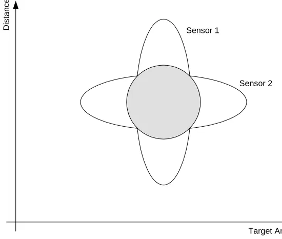
The goal of many fusion systems is uncertainty reduction and this is best achieved using

sensor complementarity (Grossmann, 1998). Fig. 1 illustrates the fusion of two sensors

used to measure distance and target angle in a mobile robot. Sensor 1 is fairly certain

about the target angle but uncertain about the range. Sensor 2 is relatively certain about

the distance but uncertain about the target range. In this case the reduction of the

measurement uncertainty is achieved by competitive fusion as both sensors measure the

same parameters.

Sensor 1

Target Angle

D

ista

n

ce

Sensor 2

Fig. 1: Fusion of complementary sensor data

A further example is the use of competitive sensor fusion for the detection of buried

(abandoned) anti-personnel landmines. No single sensor technology can reliably

achieve the detection rates demanded for humanitarian demining operations (Cremer et.

al., 1999). Consequently multisensor systems have been the subject of extensive

research and development. (Lohlein and Fritzsche, 1999) describe the fusion of a metal

detector and ground penetrating radar. The results indicate that the fusion process does

(15)

(compared with a detection probability of 63% for the metal detector and 60% for the

ground penetrating radar operated separately). Unfortunately the fused result is still

well below the UN standard of 99.6% for humanitarian demining.

Target tracking using a Kalman filter to fuse a series of measurements from a radar

system is another example of competitive fusion (Hall, 1992). In this case a single

sensor is employed, making the system vulnerable to a fault or external interference

such as jamming. Multiple sensors can be used to improve the reliability of a system

and physical redundancy has long been a feature of safety-critical systems (Napolitano

et. al., 1998b).

A great emphasis in the design of data fusion systems is that high quality data is

required from the sensors. Expressed succinctly by (Hall and Garga, 1999):

“There is no substitute for a good sensor. No amount of fusion of bad sensors will substitute for a single accurate sensor that measures the phenomenon that you want to observe.”

In many applications acting on faulty sensor data can have disastrous effects. For

example, the safe and reliable operation of complex process plant is dependent on the

reliable operation of sensors providing information about the process state (Keaton et.

al., 1998). Sensor validation is concerned with recognising when an observed value lies

outside the expected range. Two separate approaches to sensor validation have been

developed:

• Physical redundancy – Uses multiple parallel hardware sub-systems (Napolitano

et. al., 1998b);

• Analytical redundancy – Continuously monitors the sensor output signals in

order to provide fault detection. Many validation schemes use a model of the

plant or system. The model may be analytical or empirical. A sensor fault is

signalled when the measured value differs significantly from the value predicted

by the model (Patton et. al., 1995).

It is therefore apparent that important links exist between the fields of multisenor fusion

(16)

• The use of physical redundancy to provide sensor validation is a form of

competitive sensor fusion;

• Many sensor fusion and sensor validation schemes require models of sensor

performance;

• The performance of a multisensor fusion scheme is critically dependent on the performance of the individual sensors.

The central aim of this research programme is therefore to investigate the

complementary aspects of multisensor fusion and sensor validation in order to better

exploit the apparent synergy between these two activities.

1.2) Aims of the Research Programme

The aims of the research programme are:

1. To review existing schemes for multisensor fusion and sensor validation;

2. To investigate techniques used by sensor fusion and sensor validation schemes

to characterise sensor performance, in particular the use of empirical models of

sensor performance;

3. To propose new methods for the fusion of complementary sensors to provide

uncertainty reduction and improve system reliability, with particular emphasis

on the measurement of pH using thick film sensors;

4. To contribute to current knowledge by developing new schemes for sensor

validation and fusion suitable for both complementary and competitive fusion.

Such work is important because sensors play a vital role in a wide range of application

areas. The work has resulted in the following original contributions to knowledge in the

fields of multisensor fusion and sensor validation:

• The N-W estimator has been used to fuse an array of complementary thick film

(17)

robust, however they are generally manufactured in a batch process. Despite

careful control of the manufacturing process it is very difficult to achieve

reproducibility between batches. pH sensors are also susceptible to

environmental conditions and hence reliable analytical models of sensor

performance are difficult to obtain. The N-W fuser design is based on

experimental data and should be suitable for all sensors produced in a particular

batch. The N-W estimator has previously found only limited use as a fuser and

this is a new application of the technique. An empirical design procedure for the

N-W fuser has been formulated, although this manual design process can be

rather time-consuming. A Genetic Algorithm (GA) has therefore been used to

automate the fuser design process. This is a new approach to the design

optimisation of the N-W fuser.

• The N-W estimator has been used as the basis of a new sensor validation and

fault accommodation scheme. The technique makes use of sensor (physical)

redundancy. The operational characteristics of this novel approach have been

investigated and the algorithm validated using the full range of typical sensor

fault conditions.

• A fuzzy sensor validation scheme has been devised. The on-line sensor status

output is derived from change detection parameters based on spectral analysis of

the sensor output signal. This new method has been validated for all typical

sensor fault conditions and can be applied to a wide range of sensor types.

Portability is facilitated by the procedure that has been developed to

parameterise the fuzzy sets employed for fault detection using data obtained

from a healthy sensor.

1.3) Structure of the Thesis

The remaining material in this thesis is divided into the following major sections:

• Chapter 2 – Reviews the major taxonomies and architectures applicable to

multisensor fusion. Relates the main mathematical tools and techniques, giving

(18)

• Chapter 3 – Reviews the principles and applications of sensor validation

schemes based on physical and analytical redundancy;

• Chapter 4 – The N-W kernel estimator and the feedforward neural network are

employed to fuse an array of complementary thick film pH sensor electrodes.

An empirical design procedure for the N-W fuser is presented. A GA is also

employed to optimise the fuser design;

• Chapter 5 – Presents the design and evaluation of a novel sensor validation and

fusion scheme using the N-W kernel estimator;

• Chapter 6 – Proposes a sensor validation scheme using analytical redundancy to

provide on-line status information. The fuzzy status output, µ_H ∈[0,1] is potentially more useful than the simple binary status bit provided by many

sensor validation schemes;

• Chapter 7 – Discusses the model-free sensor validation and fusion schemes, and

the original contribution to knowledge, with suggestions for further work;

• Chapter 8 – Conclusions.

Extensive testing and evaluation of the various algorithms has been carried out,

principally using the MATLAB software. The results presented in the thesis have been

carefully selected to demonstrate the strengths and weaknesses of the various methods.

1.4) Concluding

Remarks

Sensors are used increasingly and in a divergent range of applications. Two separate

schemes have been developed to safeguard and enhance the quality of sensed data:

sensor fusion combines separate readings, while sensor validation confirms whether the

measured value is within acceptable limits. This research considers the complementary

aspects of these two activities and presents novel schemes that help to derive maximum

(19)

2) Multisensor Data Fusion

2.1) Definition of Multisensor Data Fusion

A useful definition of multisensor data fusion has been proposed by (Varshney, 1997a):

“Multisensor data fusion refers to the acquisition, processing, and synergistic combination of information gathered by various knowledge sources and sensors to provide a better understanding of the phenomenon under consideration.”

Another definition is due to (Wald, 1998):

“Data fusion is a formal framework in which are expressed means and tools for the alliance of data originating from different sources. It aims at obtaining information of greater quality; the exact definition of ‘greater quality’ will depend upon the application.”

This second definition emphasises the notion of combining information from various

sources to garner information of better quality than would otherwise be available using

the sources independently. The term ‘greater quality’ is used in a general sense to

indicate that the fused information should be in some way more useful to the user.

Much of the early work in the field of information fusion is related to military

applications; for example automated target tracking and recognition systems, remote

sensing, battlefield surveillance and automated threat recognition systems. A range of

non-military applications have also been developed, in particular condition monitoring

of industrial equipment, remote sensing, robotics and medical diagnosis (Waltz and

Llinas, 1990).

Data fusion draws upon a range of techniques and disciplines: digital signal processing,

statistical estimation, control theory, artificial intelligence and numerical methods. A

significant feature of the data fusion process is that information may be gathered from a

variety of sources: sensors, databases or humans. The potential advantages of a

multisensor system include (Varshney, 1997a):

• Improved reliability and robustness – there is an inherent redundancy due to the

(20)

• Extended coverage – use of multiple sensors may increase both spatial and

temporal coverage;

• Increased confidence – use of multiple sensors may help confirm inferences

from individual sensors;

• Shorter response time – because more data is collected by multiple sensors, a prescribed level of performance may be attained in a shorter time;

• Improved resolution – the overall resolution attained may be better than any

single sensor.

A practical problem is that combining accurate (good) data with inaccurate or biased

data, especially if the uncertainties or variances of the data are unknown, may actually

produce worse results than could be achieved by taking the most appropriate (best)

sensor in a suite (Hall and Llinas, 1997).

2.2) The Data Fusion Process

The following generic types of sensor fusion are defined by (Brooks and Iyengar,

1998):

• Complementary fusion – fusion of several disparate sensors that each give only

a partial view of the environment. This type of session resolves incompleteness

of sensor data;

• Competitive fusion – fusion of uncertain sensor data from several sources,

predominantly in order to reduce the uncertainty of the measurements. Fusion

can be performed on several measurements from different sensors, or on a series

of measurements from the same sensor;

• Cooperative fusion – fusion of independent sensors in order to derive an

estimate of some secondary parameter. An example given by (Durrant-Whyte,

1988) is the fusion of the ‘left’ and ‘right’ channels in a stereo vision system to

(21)

This taxonomy is very similar to the classes of sensor fusion proposed by (Tanner and

Loh, 1992):

• Uniquely determined dependent data fusion – there is precisely enough data to

determine the fused value. Tanner and Loh use the measurement of wind chill

factor from air temperature and wind speed as an example. This is

complementary fusion;

• Over determined dependent data fusion – occurs when there is more data

available than is actually required to determine the fused value. An example of

this is target tracking using data from multiple spatially dispersed radar systems.

The inherent sensor redundancy can be employed to detect erroneous sensor data

and provide reliable operation in the event of the failure of an individual radar,

due for example, to electronic counter measures. This is a competitive fusion

system.

• Under determined dependent sensor fusion – takes place when there are

insufficient sensory data to determine the desired value. This is really a process

of estimation or extrapolation. An example cited by Tanner and Loh is the

estimation of the velocity of an object from distance measurements. The

calculated velocity will only be correct if the object moves directly towards or

away from the range sensor.

A key issue is to decide where in the data flow to actually combine or fuse the data.

This fundamental design choice affects the quality of the fused product, the nature of

the algorithms or techniques employed, the complexity of the processing, and the

bandwidth of the communications required between the sensors and fusion centre (Hall

and Llinas, 1997). The choice of architecture depends on the nature of the sensors

involved, as well as the nature of the inferences sought (Hall, 1992). The main

architectures are illustrated in Fig. 2.

In Data Level Fusion (Fig. 2c) raw data from the sensors are combined. This approach

is centralised and yields the best overall results, however the sensor data are required to

be commensurate, that is observations of the same or similar physical properties, and

(22)

Feature Level Fusion (Fig. 2b) uses feature vectors extracted from sensor observations

and subsequently fused. Data communication requirements are reduced, however the

result is less accurate due to the information loss associated with generating the feature

vectors.

In Decision Level Fusion (Fig. 2a) a separate decision is produced for each sensor.

These decisions are then combined to yield the final result. The sensors need not be

commensurate and the communication bandwidth requirements are greatly reduced.

This is the least accurate of the three fusion options due to the information loss

associated with generating feature vectors and other processing.

The Data Fusion and Data Processing Technology Working Party of the Defence and

Aerospace Foresight Panel (Defence and Aerospace Foresight Technology Working

Party, 1997) also adopted a three level model of the fusion process (Fig. 3). Low level

fusion combines raw data from the sensors (data level fusion), while medium level

fusion combines features or patterns extracted from the sensed data (feature level

fusion) and high level fusion combines probabilistic information about states or

(23)

Feature Extraction Sensor A Sensor B Sensor N Identity Declaration Association I/DA I/D_B Identity Declaration Identity

Declaration I/DN

Joint Identity Declaration Decision Level Fusion . . . . . .

Fig. 2a: Decision Level Fusion [Source: (Hall, 1992)]

Feature Extraction Sensor A Sensor B Sensor N Association Joint Identity Declaration Feature Level Fusion . . .

Fig. 2b: Feature Level Fusion [Source: (Hall, 1992)]

Association Sensor A Sensor B Sensor N Data Level Fusion Joint Identity Declaration Feature Extraction . . . Identity Declaration

(24)

Sensing Signal Processing Data Feature Extraction Pattern Processing Situation Assessment Decision Making Low Level Medium Level High Level Instruction Outside World Signal Processed Signal Pattern State Probability Option Costs

Fig. 3: A model of the fusion process [Source: (Defence and Aerospace Foresight Panel Technology Working Party, 1997; Harris et. al., 1998)]

The multisensor data fusion paradigm due to (Manyika and Durrant-Whyte, 1994),

illustrated in Fig. 4, models the data fusion process as a series of data/information flows

and processing elements. A three level model of the fusion proves is again adopted,

with data, feature and decision level fusion

Feature Extraction D a ta A sso ci a ti o n Env ir o nm en t Hypothesis/ Proposition Formulation Data Level Fusion Decision Level Fusion Feature Level Fusion Inference and Estimation Decision Strategy and

Feedback Control Sensor

Sensor

To Higher Level Functions (Situation

and Threat Assessment

(25)

Many authors model fusion as a three level process (Hall, 1992; Manyika and

Durrant-Whyte, 1994; Thomopoulos, 1989; Waltz and Llinas, 1990). An alternative

characterisation of the three level fusion model has been proposed by (Dasarathy, 1997)

and is based on the input-output modes of the fusion process:

• Data In – Data Out fusion: This is commonly referred to as data fusion. Fusion

takes place at the front end of the processing stream, typically using signal or

image processing techniques. The registration, both temporal and spatial, of the

data is critical as the raw information streams from the different sensors are

combined.

• Data In – Feature Out fusion: Data from different sensors are combined to derive some feature of the object or environment. An example is the fusion of

the information gathered from each of the two sensors in a stereo vision system.

In this case the fusion process will yield depth information.

• Feature In – Feature Out fusion: Referred to as feature fusion, derived features

are extracted from the raw sensor data and combined using qualitative or

quantitative techniques.

• Feature In – Decision Out fusion: Here the inputs are features from different sensors and the output of the fusion process is a decision. This is a widely used

fusion paradigm and is used in many pattern recognition systems.

• Decision In – Decision Out fusion: Typically referred to as decision fusion. The

fusion process integrates decisions made by single or multiple sensors at the

local level. The use of multiple sensors at the local level may imply the use of

one or more of the fusion modes described above.

The fusion architecture for a Data In – Decision Out system is generally regarded as

similar to Feature In – Decision Out fusion.

This initial taxonomy is presented as the building blocks of more complex fusion

systems. In general researchers believe that fusion of information at the lowest possible

(26)

or make decisions using the sensed information may result in information loss. The low

level information may, however, suffer the highest corruption due to noise.

2.2.1) The Joint Directors of Laboratories (JDL) Model

In an attempt to codify the terminology related to data fusion, the defence communities

in the USA established a Joint Directors of Laboratories (JDL) Data Fusion Working

Group in 1986. Although the group focussed on military applications, the Data Fusion

Lexicon and model (Fig. 5) for the data fusion process established by this group are

applicable to other application areas (Hall and Llinas, 1997).

Source Pre-processing

Level One Object Refinement

Level Two Situation Refinement

Level Three Threat Refinement

Sources

Database Management

System

Human Computer

Interface

Level Four Process Refinement

Data Fusion Domain

Fig. 5: The JDL Model of the Data Fusion Process [Source: (Hall and Llinas, 1997)]

Sources – These include sensors and other a-priori information available from humans

and databases.

Human Computer Interface (HCI) – This allows human input such as commands,

information requests and human assessments of inferences. In addition the HCI is used

to communicate results to the user.

Source Pre-processing – Provides a means of regulating the flow of information

entering the data fusion system. The fusion system may easily become overwhelmed by

data from multiple sensors. Preliminary signal processing may be used to sort and

prioritise data for subsequent processing.

Level One Processing (Object Refinement) – Fuses data in order to obtain the position,

velocity and identity of low-level entities or activities. Level One processing combines

positional and identity data from multiple sensors to establish a database of identified

(27)

four separate functions: (1) data alignment, (2) data association, (3) tracking, and (4)

identification.

Level Two Processing (Situation Refinement) – Seeks a higher level of inference about

Level One processing. Both formal and heuristic techniques are used to examine the

objects and events identified by Level One processing.

Level Three Processing (Threat Refinement) – Projects the current situation into the

future in order to draw inferences about threats and opportunities. Level Three

processing develops alternate hypotheses and evaluates these in the context of the

available information.

Level Four Processing (Process Refinement) – A meta-process, concerned with the

other processes, that undertakes three key functions: (1) monitors the data fusion

process to provide information about long term performance, (2) identifies what

information is needed to improve the fusion product, and (3) allocates and directs

sensors and other assets to collect the required information.

Database Management – An important ancillary function. The database management

system is required to provide data retrieval, storage, archiving, compression and

relational queries. This task is particularly difficult because of the large and varied data

managed. A summary of the JDL data fusion process components is shown in Table 1.

The JDL process model is widely used as a conceptual framework for the data fusion

process in military and non-military applications. The separation of processes into four

separate levels is rather artificial as a real data fusion system will interleave these

(28)

SOURCES The sources provide information in a variety of levels ranging from sensor data to a priori information from databases or human input. PROCESS ASSIGNMENT Source pre-processing enables the data fusion process to concentrate on

the data most pertinent to the current situation as well as reducing the data fusion processing load. This is accomplished via data pre-screening and allocating data to appropriate processes.

OBJECT REFINEMENT (Level 1)

Level 1 processing combines locational, parametric, and identity information to achieve representation of individual objects. Four key functions are:

• Transform data to a consistent reference frame and units;

• Estimate or predict object position, kinematics, or attributes;

• Assign data to objects to permit statistical estimation; and

• Refine estimates of the objects identity or classification. SITUATION

REFINEMENT (Level 2)

Level 2 processing attempts to develop a contextual description of the relationship between objects and observed events. This processing determines the meaning of a collection of entities and incorporates environmental information, a priori knowledge, and observations. THREAT REFINEMENT

(Level 3)

Level 3 processing projects the current situation into the future to draw inferences about enemy threats, friendly and enemy vulnerabilities, and opportunities for operations. Threat refinement is especially difficult because it deals not only with computing possible engagement outcomes, but also assessing an enemy’s intent based on knowledge about enemy intent, doctrine, level of training, political environment, and the current situation.

PROCESS REFINEMENT (Level 4)

Level 4 processing is a meta-process, i.e. a process concerned about other processes. The three key Level 4 functions are:

Monitor the real-time and long term data fusion process;

Identify information required to improve the multi-level data fusion product; and

Allocate and direct sensors and sources to achieve mission goals. DATABASE

MANAGEMENT SYSTEM

Database management is the most extensive ancillary function required to support data fusion due to the variety and amount of managed data, as well as the need for data retrieval, storage, archiving, compression, relational queries and data protection.

HUMAN-COMPUTER INTERACTION

In addition to providing a mechanism for human input and

communication of data fusion results to operators and users, the human-computer interaction (HCI) includes methods of directing human attention as well as augmenting cognition, e.g. overcoming the human difficulty in processing negative information.

Table 1: JDL Process Model [Source: (Hall and Llinas, 1997)]

2.3) Architectures for Multisensor Data Fusion

The development of distributed sensor networks was originally motivated by their use

in military surveillance applications. A typical system will combine data from local

sensors, for example sonar, radar and infrared (Viswanathan and Varshney, 1997). An

alternative approach (Agre and Clare, 2000) uses many low cost spatially dispersed

(29)

of low cost sensor nodes with embedded signal processing, wireless communications,

power sources and synchronisation. Sensor nodes may be required to operate

unattended for several weeks or months. Applications include area surveillance and

environmental monitoring, where sensor nodes may be hand-emplaced, air-dropped or

munition-deployed. The distributed sensor network approach can be used to build

robust networks capable of sensing a remote area, with sensors in close proximity to the

object of interest.

The following main fusion architectures are identified in the literature:

• Centralised - sensor data are sent unprocessed from sensors and processed

entirely within the central hub of the system. The communication system may

require a large bandwidth.

• Hierarchical – intermediate processing units situated between the sensors and central hub perform pre-processing tasks.

• Blackboard – sensor nodes are essentially autonomous but exchange information

through a blackboard system.

• Decentralised – uses autonomous sensor nodes with on-board processing and

communication facilities. The system consists of a network of nodes, either

fully connected, or connected to only local nodes. The decentralised data fusion

paradigm offers a number of advantages, including modularity, scalability and

fault tolerance (Durrant-Whyte et. al., 1998).

Some important general properties of the architecture of a multisensor fusion system are

identified by (Harris et. al., 1998) and include:

• Modularity – built up from discrete modules that may be interchanged as

needed.

• Parallelisation – the computational load may be high, hence multiple processing

elements can help achieve the necessary real-time operation.

• Scalability – the system may be applied to problems of increasing magnitude

(30)

• Robustness/survivability – graceful performance degradation in the event of a

system failure is particularly important in a safety critical or military application.

• Interoperability – allow integration of different technologies i.e. an open system

design philosophy.

The majority of operational multisensor fusion systems are limited in scope and often

employ just two sensors (Grossmann, 1998). Therefore, despite the many potential

advantages of the distributed architecture, the majority of existing multisensor fusion

systems employ a centralised approach (Valet et. al., 2000).

2.4) Tools and Techniques for Multisensor Data Fusion

2.4.1) Probabilistic Methods

Bayes’ Theorem

Probabilistic methods use statistical inference techniques to compute the probability of a

hypothesis. A number of methods of hypothesis testing are identified in the literature

and described by (Hall, 1992) and (Gros, 1997). Classical inference techniques may be

generalised to include data from multiple sensors, however only two hypotheses may be

assessed at a time. Probability theory also requires a priori information about

probability density functions that may not be readily available. Consider the use of

Bayes’ theorem, named after the eighteenth century British cleric the Rev. Thomas

Bayes (1702-1761). Bayes’ theorem is used to find the a posteriori probability of

hypothesis Hi being true given the evidence E. The theorem is expressed

mathematically in the form:

∑

= i i i i i i H P H E P H P H E P E H P ) ( ) | ( ) ( ) | ( ) |

( (2.1)

where H0, H1,… Hj represent mutually exclusive and exhaustive hypotheses

P(Hi) is the a priori probability of Hi being true

(31)

Bayes’ theory provides a determination of the hypothesis being true. It is necessary to

enumerate all possible hypotheses in advance. Bayes’ theorem incorporates a priori

knowledge about the likelihood of a hypothesis being true, however when no a priori

information is available the ‘principle of indifference’ can be used where the P(Hi) are

assumed equal for all i.

Bayesian classification is employed by (White et. al., 1999) to assist with tracking of

targets in close proximity. Military systems fuse various combinations of radar, optical,

infra-red, acoustic, magnetic, radiometric and electronic surveillance data. Attributes

measured by these sensors include speed, range, altitude and radar cross-section. The

target attribute data are used to associate a target with some particular track and hence

assist the tracking algorithm. Target types are represented via a probability matrix:

P(i|j) is the probability that the sensor will declare a target of type j to have attribute i.

The Bayesian classification scheme is used to report the target belonging to the class

that has the highest probability. It is necessary to define all the target classes and

probabilities in advance. White et. al. report good results when the probability matrix is

initialised with the distributions used to generate the simulation data, however even

relatively small deviations from these exact values cause significant performance

degradation.

Kalman Filter

The Kalman filter is an algorithm for recursively estimating the state of nature given a

set of uncertain observations. The filter provides estimates of the state that are optimal

in the statistical sense (Manyika and Durrant-Whyte, 1994).

The algorithm basically consists of two steps and is often referred to as a

predictor-corrector filter. Consider the linear system described by the state equations:

) ( ) ( ) ( ) 1 ( ) 1 ( ) ( k k k k k k v Cx y w Ax x + = − + − = (2.2)

where w(k) is the process noise which is assumed to be Gaussian with zero-mean and

covariance Q(k), v(k) is the measurement noise which is assumed to be Gaussian with

zero-mean and covariance R(k), A is the state matrix of the system and C is the

(32)

Predictor equation

[

( ) ˆ( 1)

]

) ( ) 1 ( ˆ ) 1 (

ˆ k+ k =Ax kk− +G k y k −Cx kk−

x (2.3a)

Predictor gain

[

]

1

) ( )

1 ( )

(k =AP kk− C CP kk− C +R k −

G T T (2.3b)

Prediction mean-square error

[

( )

]

( 1) ( )

) 1

(k k A G k CP kk A Q k

P + = − − T + (2.3c)

The Kalman filter is frequently used to estimate the position, velocity and acceleration

of a target relative to some frame of reference by fusing sequential sensor readings. In a

system with multiple sensors it is possible to fuse the estimates produced by the

individual Kalman filters using a simple weighted sum approach (Harris et. al., 1998).

The use of Kalman filters to validate and fuse the readings from radar, sonar and optical

sensors for vehicle control on an automated highway is discussed by (Agogino et. al.,

1995) and (Goebel and Agogino, 1996). A model-based approach has been adopted. A

Kalman filter is used to estimate the measurand from the sensor readings and this value

is then compared with a model for the vehicle state. Readings are classified as faulty if

they are inconsistent with the model, although reliable validation is only possible when

the vehicle is in a state for which a model exists. Despite this, and the limitations of the

Kalman filtering algorithm, the authors report some good results based on simulation

and practical testing.

A model-based approach has also been adopted by (Julier and Durrant-Whyte, 1996)

who use a Kalman filter to temporally fuse a number of process models that describe the

behaviour of a system. The Kalman filter is used to fuse the predictions of each model

as if they were sensor information. The authors demonstrate that this approach is

theoretically sound when applied to linear systems.

The Kalman filter is perhaps the most widely used method of state estimation, however

the filter model assumes the process noise, w(k) and measurement noise, v(k) are

sequences of zero-mean Gaussian white noise with covariances R(k) and Q(k)

respectively. In many real applications the actual values of R(k) and Q(k) are not

(33)

large bound. Fuzzy control principles can be employed to adapt the behaviour of the

filter and so prevent divergence (Sasiadek and Hartana, 2000; Lho and Painter, 1993).

Other authors report good results using neurofuzzy techniques (Doyle and Harris,

1996). The reliance on stationary Gaussian models of process and measurement noise,

or alternatively a complex adaptive control scheme, is a major limitation.

Blind Source Separation

Blind Source Separation (BSS) has been used to recover the waveforms of unobserved

‘sources’ from observed measurements obtained from a Hall effect sensor array

(Paraschiv-Ionescu et. al., 1999). Expressed in matrix form:

) ( )

(t As t

x = (2.4)

where x is the vector of sensor output signals, A is the unknown ‘mixing matrix’ and s

is the vector of unknown source signals. The BSS algorithm consists of estimating a

‘separating’ matrix B either ‘on-line’ or by means of a batch algorithm:

) ( ) ( ) ( ) ( ) (

ˆ t B t x t B t As t

s = = (2.5)

This simple model can be extended in several ways:

• Unknown number of sources

• Noisy observations x(t)=As(t)+n(t)

• Non-linear mixture where is any unknown

inversible non-linear function.

⎟⎟ ⎠ ⎞ ⎜⎜ ⎝ ⎛ =

∑

= m j j ij i

i t f a s t

x

1

) ( )

( fi

( )

⋅

The technique is independent of sensor type and can be extended to non-linear sensor

behaviours. The optimisation procedure for estimating the separation matrix B may be

implemented using a neural network. At most one of the source signals is allowed to

have a Gaussian distribution. It is therefore impossible to separate two or more

Gaussian sources from each other. The performance of the algorithm may be improved

(34)

Nadaraya-Watson Estimator

A regression curve describes a general relationship between an explanatory variable Y

and a response variable X.

If n data points

{

have been collected, the regression relationship can be

modelled as:

}

n i i i Y

X , ₌₁

( )

i i i mY

X = +ε (2.6)

where m is the unknown regression function and ε_i are observation errors1. In most cases X denotes the (scalar) response variable and Y is a vector. The aim of regression

analysis is to produce a reasonable approximation to the unknown function. This can be

done essentially in two ways: parametric estimation and non-parametric estimation.

In parametric estimation the response function is approximated by some predefined

functional form, for example a polynomial regression equation. Non-parametric

estimation does not utilise a fixed parametric model.

The Nadaraya-Watson (N-W) kernel estimator is a non-parametric estimation technique

applicable to univariate and multivariate problems. Applications include engineering,

econometrics and mathematics (Blundell and Duncan, 1998; Hardle, 1990). Estimation

of the function at a particular point y is performed using the mean of observations Xi

that correspond to Yi in the region of y. In practice this estimate may be very poor if

observations are included that are distant to y since this will introduce bias. A kernel

function is therefore employed to weight the observations. As a result of the local

averaging procedure the regression estimator is often called a smoother.

1

Some sources (i.e. (Hardle, 1990)) define the regression relationship as Yi =m

( )

Xi +εi however the

(35)

The N-W estimator is given by:

(

)

(

)

∑

= = − − = _n i i h i n i i h n h Y y K X Y y K y f 1 1 , ( )

ˆ _(2.7)

where K is the kernel function and h is the bandwidth parameter. A number of kernel

functions are used in practice, for example the Gaussian function. The value of h

controls the weighting of the observations with respect to their distance to y. With a

fixed sample size the value of bandwidth h determines the degree of smoothing.

Choosing a small value of h will include only a few observations in the computation of

the estimate and may lead to a large variance. Conversely, a large value of h may

produce a significant approximation bias.

(Rao, 1997) demonstrates the use of the N-W estimator with Haar kernels to estimate a

fusion rule in a multisensor system. In a system with N sensors, the sensor Sj,

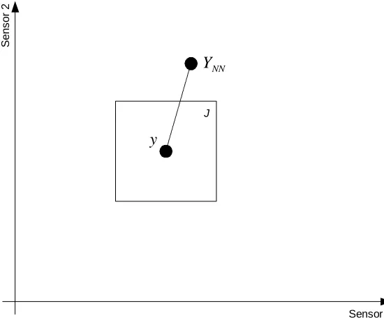
j=1,2,…N, outputs , according to an unknown probability density for the input .

The Haar kernel function is an N-dimensional hypercube, J centred on y, and having

volume , where h is the bandwidth parameter.

j i

Y X_i

N

h

The N-W estimator based on Haar kernels is therefore:

∑

∈ = ) ( 1 ) ( ˆ , i J J Y i n h Y X y f i (2.8)

where denotes the indicator function 1_J(Y_i)

⎩ ⎨ ⎧ ∈ = otherwise J Y if

Y_i i

J 0 1 ) ( 1

Computation of fˆ_h_,_n(y) at any given y involves obtaining the local sum of Xi’s in J and

this is the key to the efficient computation of the estimate. If no Yi’s lie in J then

is taken to be zero. In order to reduce the complexity of the estimator, and also

the time required to compute the estimate, it is desirable to minimise the number of

a-priori observations employed. Using few observations suggests that a large value of h )

( ˆ

, y

(36)

will be needed to ensure at least one Yi lies in J for all y and this will increase the

approximation bias.

The classical N-W estimator is shown to effectively perform data and decision-level

fusion (Rao, 1999). Data-level fusion is illustrated using the N-W estimator to fuse five

noisy estimates of an unknown function. The statistical estimator is shown to perform

better than a feedforward neural network using training sets of 100, 1000 and 10,000

input-output pairs. The N-W estimator is also shown to fuse an array of four ultrasonic

and four infrared sensors fitted to a mobile robot. The sensors are employed to measure

the width of a door or similar opening to check that the gap is large enough for the robot

to pass through. The infrared sensors are susceptible to surface texture and the colour of

the walls, while the ultrasonic sensors are susceptible to multiple reflections. It is very

difficult to derive accurate probabilistic models of the sensors, however experimental

data are relatively easy to obtain. The training data included 6 positive examples

(opening wide enough) and 12 negative examples (opening not wide enough). During

testing the N-W estimator correctly classified the width of an opening for all examples

of the test data, however Rao does not describe the design procedure that was adopted

for the estimator.

2.4.2) Dempster-Shafer Theory

Dempster and Shafer created a generalised form of the Bayesian inference model

(Shafer, 1976). This method seeks to assign measures of belief to combinations of

hypotheses.

Assume a set of mutually exclusive and exhaustive propositions:

{

0, 1, 2,... −1

}

=

Θ X X X XN (2.9)

where Θ is called a ‘frame of discernment’ in Dempster-Shafer terminology.

It is possible to develop (2N-1) general propositions from Boolean combinations of the original set, i.e.

{

∨ ∨ Θ

}

=

Θ ~

,... ,

,

(37)

The concept of probability mass is employed to assign evidence to a proposition. Any

belief not assigned to a specific proposition is called a non-belief and is associated with

Θ~ .

The probability masses m(X0), m(X1), m(X0∨X1) etc. are assigned such that

and . Note that m(Θ) denotes a probability mass assigned either to an elementary proposition (i.e. m(X

] 1 , 0 [ ) (Θ →

m

∑

m(Θ)=1

0), m(X1), etc.) or to a general proposition in

the set 2Θ.

The support for a hypothesis X is defined by the belief function:

∑

⊆ = X X i i X m X

Bel( ) ( ) (2.11)

This is the sum of the probability masses assigned to the proposition. Thus if X is a

general proposition, Bel(X) is the sum of the probability masses contributing to all

elements of X, i.e. Bel(X0 ∨ X1)=m(X0)+m(X1)+m(X1∨ X2).

The plausibility of a hypothesis X is defined by:

∑

⊄ − = − = X X i i X m X Bel X

Pls( ) 1 ( ) 1 ( ) (2.12)

Thus the plausibility of a proposition is the sum of all the masses not assigned to its

negation.

The properties of the belief function include:

1 ) (Θ =

Bel as

∑

Θ ⊆

=

x

X m( ) 1

0 ) (Θ =

Bel if X ⊄Θ

Data association using Dempster-Shafer theory is performed using the Dempster rule of

(38)

c Y m X m Z

m X Y Z

− =

∑

∩ = 1 ) ( ) ( ) ( 2 1 (2.13)

where

∑

and φ denotes the empty set.

= ∩ = φ Y X Y m X m

c ₁( ) ₂( )

The normalisation factor, c is the sum of the products of masses assigned to conflicting

propositions.

The result of the Dempster rule of combination is a set of evidential intervals [Bel(Z),

Pls(Z)], where Bel(Z) is the belief assigned to the proposition Z and Pls(Z) is the

plausibility of Z. This is represented diagrammatically in Fig. 6.

Region of Uncertainty

0 1

Disbelief Belief

Plausibility

Fig. 6: Illustration of evidential intervals

Dempster-Shafer theory considers belief in sets of possibilities instead of considering

each possibility separately. This makes rules easier to write. The result is a range of

beliefs for each proposition. Dempster’s rules of combination are both commutative

and associative, and consequently parallel implementations are possible.

Critics of Dempster-Shafer theory note that the Dempster rule of combination may yield

counter-intuitive results in certain circumstances (Murphy, 1998; Zadeh, 1986).

Consider the case where one of three possible propositions, X0, X1 or X2 must be true

and Sensor 1 provides evidence: m(X0)=0.7, m(X2)=0.3, while Sensor 2 provides

contradictory evidence: m(X1)=0.8, m(X2)=0.2. Dempster’s rule of combination will

give the following results: Bel(X0)=0, Bel(X1)=0 and Bel(X2)=1. Thus indicating

complete support for hypothesis X2. The normalisation factor, c can therefore be

viewed as a measure of conflict between belief functions.

Dempster-Shafer theory is commonly used to provide decision level fusion. An

example of Dempster-Shafer fusion applied to a vision system is described by (Murphy,

1998). The evidence of a feature is based on how well the observed value of the feature

(39)

goodness-of-fit function that was adapted to assign belief to a particular proposition. The weight of

conflict metric, which quantifies discordance in a set of evidence, can be used to

indicate a possible sensor failure. In such cases heuristic domain knowledge may be

employed to enact some form of coping strategy.

(Cremer et. al., 1999) evaluate the use of Dempster-Shafer theory to fuse data from a

metal detector, infrared camera and ground-penetrating radar in order to detect the

presence of buried antipersonnel landmines. After acquisition, the data from the

individual sensors are processed and mapped to obtain decision-level data on a

reference grid. The confidence value on each cell expresses a confidence or belief in

the presence of a landmine at that position. The confidence value has a high correlation

with the associated probability but no statistical meaning. The individual sensors are

then fused using Dempster-Shafer theory. Experimental results demonstrate that the

fusion scheme performs better than the best single sensor. The use of decision-level

fusion in this case is necessary because it is not possible to directly fuse the disparate

raw data streams from the various sensors.

2.4.3) Fuzzy Logic

Fuzzy set theory was first introduced by (Zadeh, 1965) as an extension to the crisp set.

The crisp set A can be defined using the indicator function:

⎩ ⎨ ⎧

∉ ∈ =

A x if

A x if x

A

0 1 ) (

µ (2.14)

In contrast a fuzzy set is defined by a membership function µ_A(x) that takes values in the range [0,1]. Fuzzy systems provide a convenient mechanism for transforming a set

of linguistic rules into a non-linear mapping. The first fuzzy control application was

presented by (Mamdani and Assilian, 1975). The controller used four inputs: Pressure

error, Speed error, Change in pressure error and Change in speed error; and two outputs:

Heat change and Throttle change. The controller employed 24 rules and consistently

gave better results than a fixed digital controller when used to regulate a steam engine

and boiler combination. Fuzzy systems have since found their way into a variety of

engineering applications. In practice the rules are often ‘guessed’ by human experts or

(40)

rule base and membership functions is generally necessary in order to achieve the

desired performance (Kosko, 1997).

Fuzzy systems provide an effective model-free method of approximating a non-linear

function using IF-THEN rules. The rules may be derived from expert knowledge or

training data. Consequently fuzzy systems have been used in a wide range of data

fusion application areas, including robotics (Baglio et. al., 1996), manufacturing

(Karlsson et. al., 2000) and defence (Smith, 1998).

Fuzzy systems are universal approximators; that is they can approximate any non-linear

function. The fuzzy IF-THEN rules define fuzzy patches in the input-output space X×Y. The fuzzy system F: X→Y approximates a function f: X→Y by covering its graph with rule patches and averaging patches that overlap. Increasing the number of rule patches,

and hence reducing the size of the patches, has the effect of improving the accuracy of

the estimate. The rules grow exponentially in number as the dimensions of X and Y

increase. This rapid increase in the number of rules is known as “the curse of

dimensionality”. (Wang, 1997) identifies three separate situations where it may be

necessary to find an optimal fuzzy system that approximates some non-linear function,

f(x):

• The analytical formula of f(x) is known;

• The analytical formula of f(x) is unknown but for any x∈U we can determine the corresponding f(x);

• The analytical formula of f(x) is unknown but we are provided with a limited

number of input-output pairs

{

j

( )

j

}

n_j

x f

x , ₌₁ where xj cannot be arbitrarily chose

Algorithms for sensor validation and multisensor fusion

ALGORITHMS FOR SENSOR VALIDATION AND MULTISENSOR FUSION

Acknowledgements

Table of Contents

ABSTRACT ...ii

2.2) The Data Fusion Process ... 19

2.6) Concluding Remarks ... 45

4.3) Multisensor Fusion using a Feedforward Neural Network... 66

5.3) Concluding Remarks ... 85

7.4) Multisensor Validation and Fusion using the Nadaraya-Watson Kernel Estimator... 128

8) Conclusions ... 135

List of Figures and Tables

List of Figures

List of Tables

1) Introduction

1.2) Aims of the Research Programme

1.3) Structure of the Thesis

1.4) Concluding

2) Multisensor Data Fusion

2.2) The Data Fusion Process

2.2.1) The Joint Directors of Laboratories (JDL) Model

MANAGEMENT SYSTEM

2.3) Architectures for Multisensor Data Fusion

2.4) Tools and Techniques for Multisensor Data Fusion

2.4.1) Probabilistic Methods

Bayes’ Theorem

Kalman Filter

where w(k) is the process noise which is assumed to be Gaussian with zero-mean and

the filter model assumes the process noise, w(k) and measurement noise, v(k) are

Blind Source Separation

where x is the vector of sensor output signals, A is the unknown ‘mixing matrix’ and s

behaviours. The optimisation procedure for estimating the separation matrix B may be

Nadaraya-Watson Estimator

2.4.2) Dempster-Shafer Theory

2.4.3) Fuzzy Logic