Motor unit action potential
conduction velocity estimated from surface
electromyographic signals using image
processing techniques
Fabiano Araujo Soares
1,2*, João Luiz Azevedo Carvalho
1, Cristiano Jacques Miosso
2,
Marcelino Monteiro de Andrade
2and Adson Ferreira da Rocha
2Background
In surface electromyography (surface EMG, or S-EMG), conduction velocity (CV) refers to the velocity at which the motor unit action potentials (MUAPs) propagate along the muscle fibers, during contractions. MUAPs propagate in the direction that causes the membrane voltage of muscle fiber cells to approach and surpass the threshold for excita-tion, causing the action potential to move [1]. This propagation occurs along the direc-tion of the muscle fibers, and originates from the innervadirec-tion zone (IZ) in opposing directions, towards the tendinous regions. The CV is related to the type and diameter of the muscle fibers, ion concentration, pH, and firing rate of the motor units (MUs)
Abstract
In surface electromyography (surface EMG, or S-EMG), conduction velocity (CV) refers to the velocity at which the motor unit action potentials (MUAPs) propagate along the muscle fibers, during contractions. The CV is related to the type and diameter of the muscle fibers, ion concentration, pH, and firing rate of the motor units (MUs). The CV can be used in the evaluation of contractile properties of MUs, and of muscle fatigue. The most popular methods for CV estimation are those based on maximum likeli-hood estimation (MLE). This work proposes an algorithm for estimating CV from S-EMG signals, using digital image processing techniques. The proposed approach is demon-strated and evaluated, using both simulated and experimentally-acquired multichan-nel S-EMG signals. We show that the proposed algorithm is as precise and accurate as the MLE method in typical conditions of noise and CV. The proposed method is not susceptible to errors associated with MUAP propagation direction or inadequate initialization parameters, which are common with the MLE algorithm. Image process-ing -based approaches may be useful in S-EMG analysis to extract different physiologi-cal parameters from multichannel S-EMG signals. Other new methods based on image processing could also be developed to help solving other tasks in EMG analysis, such as estimation of the CV for individual MUs, localization and tracking of innervation zones, and study of MU recruitment strategies.
Keywords: Surface electromyography, Conduction velocity, Image processing
Open Access
© 2015 Soares et al. This article is distributed under the terms of the Creative Commons Attribution 4.0 International License (http:// creativecommons.org/licenses/by/4.0/), which permits unrestricted use, distribution, and reproduction in any medium, provided you give appropriate credit to the original author(s) and the source, provide a link to the Creative Commons license, and indicate if changes were made. The Creative Commons Public Domain Dedication waiver (http://creativecommons.org/publicdomain/ zero/1.0/) applies to the data made available in this article, unless otherwise stated.
RESEARCH
*Correspondence: [email protected]; [email protected] 2 UnB Gama Faculty, University of Brasília, Area Especial de Indústria, Projeção A, Setor Leste, Gama, 72444-240 Brasília, DF, Brazil
[1–5]. The CV can be used in the evaluation of contractile properties of MUs [6], and of muscle fatigue [7–9]. Typical values of CV are in the 3 to 5 m/s range, with an average of approximately 4 m/s [1]. In clinical applications, CV can be used to supplement the information at the muscle’s fiber level obtained with needle EMG [10]. For example, van der Hoven studied CV in patients with amyotrophic lateral sclerosis using needle and S-EMG and discovered that these patients presents increased CV and decreased median frequency [11].
The CV can be estimated from S-EMG signals measured using an array of electrodes, placed over the target muscle, and parallel to the muscle fibers. Signal conditioning is typically performed using four or more electrodes in a double differential configuration. This setting is used because it provides greater reduction of end-of-fiber components, when compared to the differential configuration [12]. However, the differential configu-ration may also be used to estimate the CV, especially when the detection region is far from IZs and tendon regions [13].
A current approach generally used to estimate the CV is based on computing the ratio between the interelectrode distance (IED) and the delay between the S-EMG waveforms associated with two or more adjacent electrodes [12, 14–23]. The most popular methods for CV estimation are those based on maximum likelihood estimation (MLE) in the fre-quency domain, which provide higher velocity resolution and lower variance than other approaches [12, 23]. Most of the CV estimation methods available in the literature pro-vide only a mean CV value [14–17, 20, 21, 23]. However, methods for estimating the CV associated with a single MU have also been proposed [12, 23]. In 2004, Farina et al. com-pared the MLE with these approaches and other common methods, and showed that MLE is the most accurate among them [23]. To the best of our knowledge, MLE is still the most used CV estimation method.
Two-dimensional (2D) features of multichannel S-EMG—where the two dimensions correspond to the electrode-array axis and the time axis, respectively—can be exploited to estimate the mean CV. Grönlund et al. has used 2D techniques to estimate the CV of a single MU, as well as muscle fiber orientation, using an optimal trajectory method [24]. The techniques in [25] are more precise and more usable in practice, but have some limi-tations such as poorer performance in case of MUAP superposition and requirement of a priori knowledge of the direction of propagation.
This paper proposes a 2D method for estimating the mean of the CV from electrode-array S-EMG signals, using digital image processing techniques. The proposed method is based on the processing of images constructed from the set of signals acquired with an array of electrodes, placed parallel to the muscle fiber. The analysis of such images allows the estimation of the delay between similar waveforms on adjacent S-EMG channels. Then, just as in the traditional methods for CV assessment, the CV is estimated as the ratio between IED and MUAP delay.
Methods
Multichannel S‑EMG signal displayed as an image
measured signals are stored as a matrix, in which the rows correspond to different chan-nels, and the columns correspond to different time instants (or vice-versa). Such matrix may be displayed as an image, as follows.
Acquisitions using a (M+1)-electrode array in single-differential mode will result in M-channel S-EMG signals (Fig. 1a). A N-sample segment of such a signal will corre-spond to a M×N matrix. Such a matrix may be displayed as a M×N image, by
map-ping the signal amplitude values onto a gray-scale color map. In such image, the vertical axis corresponds to the spatial position along the electrode array, the horizontal axis corresponds to time, and the gray levels represent the intensity of the measured electric potential (signal amplitude).
However, the number of channels in an array is generally not higher than 15. In this case, the image would be extremely narrow and difficult to visualize and process. This can be addressed by interpolating the multi-channel S-EMG signal along the channel axis (or along both axes), thus obtaining a matrix of a larger size, which may be more clearly visualized in image form (Fig. 1b). The interpolation in both dimensions also improves the performance of the image processing algorithm proposed in this work, by thickening the diagonal lines associated with conduction of the MUAPs, as dis-cussed below. Generally, white and light gray pixels in the resulting images represent
50 100 150
time (ms) 1
3 5 7
channel number 0
−1 0 1 normalized amplitude
0 1 normalized amplitude a
b
c
d
Fig. 1 Steps of the proposed CV estimation algorithm. a 150-ms segment of a 7-channel synthetic S-EMG
large positive amplitude values, while black and dark gray pixels represent large negative amplitude values; small amplitude values are represented by intermediary shades of gray.
The interpolated data, when displayed as a gray-scale image, allows the identification of the MUAPs, which form diagonal lines diverging from the rows associated with IZs. These lines represent the conduction of the MUAPs along the muscle fibers. The shapes of these conduction lines are affected by many morphological parameters of the corre-sponding MU, such as: (1) length and width of the MUAP line, which is associated with the depth of the MU that originated the MUAP and the number of fibers of the MU that originated the MUAP; (2) the velocity in which the MUAP travels along the MU, i.e. the CV, which is the slope of the conduction lines; and (3) the location of IZs, which may be detected as pairs of conduction lines with opposite slope, originating from horizontal gray-colored regions of the image [26]. This work, however, focuses solely on estimating the CV from the S-EMG images.
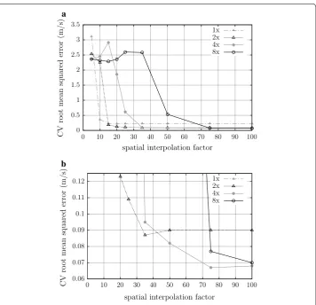
The S-EMG image associated with each multichannel S-EMG signal (or with each seg-ment of one) was constructed by resizing the 2D data using four-fold interpolation along the temporal axis, and 75-fold interpolation along the spatial (channel number) axis. These interpolation factors were chosen empirically and are the best pair for minimizing error, as can be seen in Fig. 2, this figure was created using 100 signals generated by the method described on section CV experiments using simulated S-EMG signals. Bicubic interpolation was used, as it generally does a better job of preserving fine detail than the bilinear approach [27].
MUAP‑enhancement filter
The images obtained from the multichannel S-EMG signal show several diagonal lines of varying intensity, associated with the MUAPs (Fig. 1b). Low-intensity conduction lines are generally associated with deep MUs, or with MUs of smaller size (with few mus-cle fibers). Conduction lines generally do not have mus-clear boundaries, and low intensity MUAPs may be lost if a binarization process is applied directly. In order to address this issue, a waveform-detection filter was used to intensify regions where MUAPs are present, by highlighting the edges of the conduction lines (Fig. 1c). We chose an Her-mite filter for this task—after also experimenting with Gaussian and Gabor filters—, as it allowed a better delineation of the MUAPs, for the signals we tested. This approach was first introduced by us, for both CV estimation [28, 29], and IZ detection [26, 30]. More recently, Ullah et al. used Hermite filtering for MUAP-enhancement in multi-scale S-EMG processing [31].
Let x be the horizontal axis of the S-EMG image (time), and y be its vertical axis (spa-tial position along the electrode array). The kernel of the Hermite filter is the first deriva-tive of a Gaussian with respect to the x-axis:
where σx and σy are the standard deviations (in number of pixels) about the x and y axes, respectively, and define the kernel width [32].
(1)
G2,1(x,y)= −
x
2π σ3
xσy exp
−x
2
σ2 x
− y 2
σ2 y
This filter will emphasize MUAP conduction lines that are above or below an IZ, without the need to consider the direction of propagation of the MUAPs. We used σx=σy= 60 pixels; these values are consistent with the typical duration of MUAPs [33] and proposed interpolation factors. With this configuration, the Hermite filter is able to highlight the differences between regions of inactivity and regions where MUAPs are present (Fig. 1c). These values were chosen based on a compromise between the size of the filter, and edge effects created by the filter response (ripple artifacts). We found this setting to be the most suitable for all the experiments we conducted. The proposed values can be changed according to the needs of a particular experiment or applica-tion. To validate the filter tuning, we estimate CV of 100 simulated S-EMG signals, the simulation process is described in the section CV experiments using simulated S-EMG signals. In this validation process σx and σy values were changes from 10 to 100 in steps of 5 independently, and the value of 60 for both parameters was the one that provides most precise results.
0 0.5 1 1.5 2 2.5 3 3.5
spatial interpolation factor
CV
ro
ot
mean
squared
error
(m/s) 1x2x
4x 8x
0.06 0.07 0.08 0.09 0.1 0.11 0.12
0 10 20 30 40 50 60 70 80 90 100
0 10 20 30 40 50 60 70 80 90 100
spatial interpolation factor
CV
ro
ot
mean
squared
erro
r(
m/s) 1x2x
4x 8x a
b
Fig. 2 Estimation of the root mean squared error for the IPE algorithm using 100 synthetic signals with force
Conduction velocity estimation
The proposed image processing estimation (IPE) algorithm for CV estimation is based on calculating the slope of the MUAP conduction lines on segmented S-EMG images. The algorithm consists of the following steps:
(a) The S-EMG image is constructed from a multichannel S-EMG signal (or a segment of one), using the previously described process (Fig. 1b).
(b) An Hermite filter is used to improve the contrast of the MUAP conduction lines (Fig. 1c).
(c) The image is binarized. This eliminates background noise, and allows the use of binary morphological operations. The threshold is set to the median amplitude value of the Hermite-filtered image.
(d) A morphological opening operation is performed. This operation aims to erase noisy (irregular and grainy) lines, typically associated with problematic regions of the image (e.g., motion artifacts).
(e) A morphological thinning operation is performed, in order to reduce the width of the MUAP conduction lines. Morphological thinning removes pixels from an object, until a line where all pixels are connected is obtained. This results in diagonal lines that can be used to estimate the CV (Fig. 1d).
(f) All objects shaped like the letter “H” are broken, in order to remove connections between two conduction lines.
(g) Isolated pixels are removed.
(h) The image is cropped (edges are removed), in order to avoid distortions due to filter-ing and interpolation (e.g., Gibbs artifacts).
(i) Conduction lines are automatically labeled by an object detection algorithm, which finds and labels each image element that is not connected to other elements.
(j) The slope of each conduction line is estimated, using least squares linear regression. This is the measured CV for the associated MUAP.
(k) All MUAPs with mean squared error (MSE) (with respect to the corresponding regression line in the channel direction) greater than 0.6 mm2 are eliminated. This is because lines with MSE larger than this threshold are usually associated with false, noise-related objects.
(l) Lines shorter than the value of the inter-electrode distance (5 mm) are discarded. (m) Vertical lines (slope greater than 20 m/s) are discarded. These lines do not
repre-sent MUAP propagation, and therefore must not be considered. (typical CV values ranges from 3 to 5 m/s).
Note that classification algorithms could be used (prior to binarization) to identify dif-ferent MUs, and thereby estimate the CVs of individual MUs. The shapes, intensity, and position of each MUAP could be used for this classification. We propose this idea as a potential future work.
Evaluation of the proposed algorithm
The performance of the proposed IPE algorithm was quantitatively and qualitatively evaluated by comparison with the MLE algorithm proposed by Farina et al. [12]. This algorithm estimates the CV by finding the waveform delay between adjacent channels that minimizes the MSE between the channels’ waveforms and a template signal, which is modeled as the mean of the waveforms measured on all channels, after delay compen-sation. It is important to mention that the initial CV value for the MLE algorithm was set to 4 m/s, and that we assumed that the propagation direction was known. IPE, however, does not require a choice of initial CV value, nor a priori knowledge about propagation direction; in fact, IPE estimates the CV for both directions of propagation, and does not require any kind of initialization.
CV experiments using simulated S‑EMG signals
A total of 750 synthetic signals were generated, using the simulation method proposed by Farina and Merletti [34]. Each simulated signal contains seven differential channels. The signals were designed based on a hypothetical muscle with 200 mm length, fat layer of 6 mm, skin layer with 1 mm, and 30 motor units, each with a random number of muscle fibers (ranging from 50 to 550 fibers) and MU recruitment threshold of 100 % of the MVC. All signals were simulated far from tendinous regions and innervation zones, and based on a single narrow IZ, so that the simulated MUs are innervated at the same location. The simulated IZ was positioned far from the electrodes. The sampling rate was 2048 Hz (per channel). The simulation was based on a set of 8 linear electrodes contacts with 5 mm IED. The total duration of each signal was 3 s.
These signals were separated into eighteen groups of 50 synthetic signals, which were used to compare the two algorithms. Signals from each group had different CV values (3, 4, or 5 m/s), null standard deviation, different signal-to-noise ratio (SNR) values: ∞ (noise free), 30, 20, 16, or 12 dB and different force levels (20, 40 and 60 % of the MVC). The CV for each signal from each group was estimated using both MLE and IPE rithms. The results were then quantitatively and qualitatively compared between algo-rithms, and with the true CV for each signal, by means of scatter plots and root mean squared error (RMSE) levels.
previous experiment, but performing the CV estimation process multiple times, each time with a different window length. The results were evaluated by comparing RMSE levels. Just 4 m/s noise free and 16 dB SNR signals were used for this analysis. The win-dow length used were 0.5, 0.75, 1.0, 1.5, or 3 s, the RMSE was calculated from the CV values estimated in all windows—6, 4, 3, 2, or 1 window, respectively—from all 50 sig-nals in the set.
We also analyzed the influence of the number of channels used to estimate the CV for both algorithms. The number of channels was varied between 4 and 7. In this experi-ment, the CV was 4 m/s, and the window length was 3 s, for all signals. This evaluation was performed at two different noise levels: noise-free and 16 dB SNR. The results were evaluated by comparing RMSE levels.
When analyzing the results of these CV experiments using simulated S-EMG signals, we will consider that the CV estimates are accurate and precise if (and only if) the RMSE is lower than 0.1 m/s. Such low RMSE allows evaluating statistically significant differ-ences between the CV estimates of different MUs, thus allowing the estimation of the CV of a single MU [12]. Therefore, we define our “high-goodness threshold” at 0.1 m/s. If the RMSE is higher than 0.1 m/s, but lower than 0.5 m/s, than it may not be possible to distinguish different MUs, but it is still possible to detect variations of the average CV [12]. Thus, we define our “low-goodness threshold” at 0.5 m/s; i.e., we will consider that the CV estimates are inaccurate and/or imprecise if (and only if) the RMSE is greater than 0.5 m/s.
CV experiments using biceps brachii signals
Finally, both algorithms (IPE and MLE) were used to estimate the CV in biceps brachii S-EMG signals. Twenty-three females and eighteen males volunteered to participate in the study. Due to withdrawal, hormonal problems, failing channels, fail in sustain iso-metric strength level and high levels of noise in the S-EMG recordings, only sixteen female volunteers (24.1 ± 2.5 years old) and eleven male volunteers (25.8 ± 2.6 years of age) were included in the analysis. All subjects were right-handed and had no known neurological disease. All female subjects had regular menstrual cycles, did not practice regular exercise, and were not using any medication or hormonal contraception for at least 6 months. Male volunteers also did not practice regular exercise. All volunteers read and signed an informed consent form. The experimental protocol was approved by the research ethics committee of the University of Brasília.
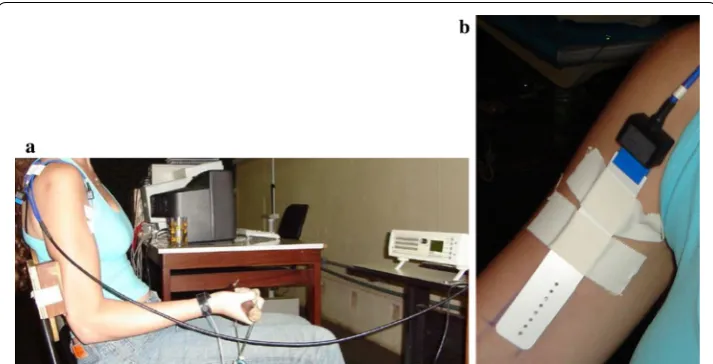
The same experimental protocol was executed with all the volunteers. Each female subject performed the experimental protocol in four sessions, with a one week interval between sessions. Male volunteers underwent a single session. Each volunteer sat on a chair, specially adapted to secure the elbow, so that the only possible movement of the arm was isometric elbow flexion (Fig. 3a). This was done to minimize muscle contrac-tions that could impact the results of the experiment.
Bioelettronica snc, Italy), was used to measure the strength level of the subjects. The amplification gain was set to 1.
Three 3-second isometric contractions were performed at the beginning of each ses-sion to determine the volunteer’s MVC. However, for female volunteers, the MVC meas-ured during the first session was adopted as the MVC for all sessions; MVC values of other acquisitions were measured only to ensure the repeatability of the protocol in all sessions. Strong verbal encouragement was used for each MVC. After each MVC esti-mation, the subject rested for 1 min.
Then, in each session, an array of 16 electrodes (Ag, size: 10 × 1 mm, 5 mm
inter-electrode distance, OT Bioelettronica snc, Italy) was used to map the ideal region of the biceps brachii muscle for the acquisition of the S-EMG signals [36]. For this assessment, the sampling rate was 2048 Hz per channel, the gain was set to 1000, an analog differen-tial configuration was used, and the strength level was 30 % of the MVC. Three-second signal acquisitions were used for mapping the ideal position. After this mapping proce-dure, the volunteer rested for two minutes.
After mapping, S-EMG signals were acquired with a semi-disposable linear array of eight surface electrodes (5 mm inter-electrode distance, OT Bioelettronica snc, Italy), which was placed on the optimal region (between IZ and tendon regions) of the biceps brachii short head (Fig. 3b). The skin was cleaned and conductive gel was applied between the skin and each electrode. The differential configuration was used, resulting in a 7-channel S-EMG signal for each acquisition. A reference electrode was placed on the right wrist. The sampling rate was 2048 Hz, and an the analog gain was set to 1000. A 10-second acquisition using 20 % of the MVC was performed. The subjects rests than for 2 min and finally, a 90-s acquisition using 40 % of the MVC was performed.
A total of 27 signals were selected from those measured during the 10-s contractions (signals from the IZ mapping procedure were not used for CV estimation tests). Signals
Fig. 3 Experimental setup. a Position of the subject during exercise. A chair was adapted so that the elbow
that presented poor quality in at least one channel—60 Hz interference, movement arti-facts, loss of electrode contact (intermittent or constant)—were discarded. The signals were not segmented (i.e., 10-s window length), and seven channels were used for obtain-ing the S-EMG images. In these experiments, the true CV is unknown. Thus, CV esti-mates obtained with the proposed method were compared with those obtained with the MLE algorithm, by means of correlation coefficient, linear regression, and scatter plots analysis.
Results
CV experiments using simulated S‑EMG signals
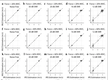
Figure 4 and Tables 1 and 2 show the results of the CV estimation comparison between the proposed IPE algorithm and the MLE algorithm proposed by Farina et al. [12], using simulated signals with different levels of noise, different CV values and different force levels.
In Fig. 4, we show MLE versus IPE scatter plots for each noise level, with groups with different nominal CV values shown in different colors in each scatter plot. The black diagonal dashed lines represent the identity line; therefore, if the dots are grouped near the diagonal line, this indicates that the two algorithms provided similar CV estimates.
Tables 1 and 2 present the same results in a different fashion, by evaluating the effects of the noise level and force level on the RMSE for each algorithm, and for each CV value.
a
f
k l m n o
g h i j
b c d e
Fig. 4 CV estimation comparison between the proposed IPE algorithm and the MLE algorithm proposed by
These results show that, when assessing signals with high SNR (≥16 dB), both methods were able to estimate the CV for all signals with high accuracy and precision (RMSE ≤
0.1 m/s) i.e. the results in this SNR range are within the high-goodness threshold defined in the methodology.
At low SNR (≤12 dB), the MLE method presented results within the
low-good-ness threshold, defined in the methodology (0.08 m/s ≤ RMSE(MLE) ≤ 0.24 m/s, with
RMSE(MLE) the root mean squared error of the MLE). In some MLE estimations it is possible to see the spreading of the estimated CV value in Fig. 4e, j, o. This is due to local minima problems associated with the Newton–Raphson method, which is used in the MLE algorithm. The proposed IPE method does not use iterative optimization methods, therefore it is not susceptible to this type of error. The IPE method has a slightly better performance for 12 dB SNR (0.05 m/s ≤ RMSE(IPE) ≤ 0.17 m/s, with RMSE(IPE) the
root mean squared error of the IPE). However, there is no spreading behavior in the IPE case, as opposed to the MLE results.
Table 1 RMSE of IPE algorithm for synthetic signals with CV equal to 3, 4, and 5 m/s, force level equal to 20, 40 and 60 % of the MVC and SNR of ∞ (noise free), 30, 20, 16 and 12 dB CV (m/s) ∞ dB SNR 30 dB SNR 20 dB SNR 16 dB SNR 12 dB SNR
Force level = 20 % MVC
3 0.02 0.03 0.04 0.04 0.05
4 0.09 0.09 0.10 0.10 0.10
5 0.03 0.03 0.04 0.09 0.14
Force level = 40 % MVC
3 0.03 0.03 0.04 0.05 0.05
4 0.09 0.09 0.09 0.09 0.08
5 0.03 0.03 0.04 0.08 0.17
Force level = 60 % MVC
3 0.03 0.03 0.04 0.04 0.05
4 0.08 0.09 0.09 0.10 0.09
5 0.03 0.03 0.04 0.07 0.12
Table 2 RMSE of MLE algorithm for synthetic signals with CV equal to 3, 4, and 5 m/s, force level equal to 20, 40 and 60 % of the MVC and SNR of ∞ (noise free), 30, 20, 16 and 12 dB CV (m/s) ∞ dB SNR 30 dB SNR 20 dB SNR 16 dB SNR 12 dB SNR
Force level = 20% MVC
3 0.03 0.03 0.04 0.04 0.15
4 0.04 0.04 0.04 0.04 0.12
5 0.05 0.05 0.05 0.06 0.15
Force level = 40% MVC
3 0.03 0.03 0.03 0.04 0.13
4 0.04 0.04 0.04 0.05 0.24
5 0.04 0.04 0.04 0.06 0.08
Force level = 60% MVC
3 0.03 0.03 0.03 0.04 0.16
4 0.04 0.04 0.04 0.04 0.08
Another important aspect we observed is the fact that the applied force level seems to have little effect on the performance of both the IPE and the MLE methods, specially for high SNRs. In fact, Tables 1 and 2 show that for signals with 30 and 20 dB, there is no difference between the measured root mean squared errors for different force lev-els, within the considered numeric precision. In the case of signals with 12 dB, there were different RMSE (for the MLE only) for different tested force levels, but the error sometimes increased and sometimes decreased with the force level. We believe that the local minimum problem previously mentioned has an impact on the MLE performance in this high-noise scenario, and we did not identify a monotonic relation between the force level and the measured error.
The results in Fig. 4 and Tables 1 and 2 were obtained from simulated S-EMG signals, using 3-s windows—i.e., the entire signal length—, and seven S-EMG-channels. We now evaluate the influence of window length and number of channels on CV estimation.
Influence of window length
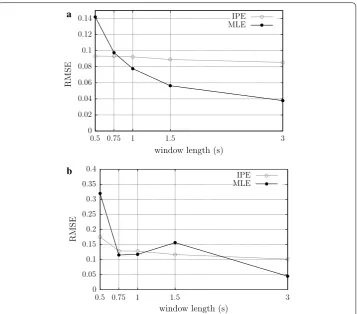
Figure 5 shows the results of the experiments which evaluated the influence of window length on CV estimation, considering a force level of 20 % of the MVC. For noise free signals, the result for the MLE shows RMSE reducing slightly as the window length
0 0.02 0.04 0.06 0.08 0.1 0.12 0.14
0.5 0.75 1 1.5 3
window length (s)
RMS
E
IPE MLE
0 0.05 0.1 0.15 0.2 0.25 0.3 0.35 0.4
0.5 0.75 1 1.5 3
window length (s)
RMS
E
IPE MLE a
b
Fig. 5 Evaluation of the influence of window lengths on CV estimation in the MLE and IPE methods, for
increases, the IPE method has a constant behavior. At 0.75 s, both algorithms have simi-lar behavior. For 16 dB SNR signals, results for the MLE and IPE algorithms were very similar, with the RMSE reducing slightly as the window length increases. Overall, the performance of the MLE method was slightly superior to that of the proposed algo-rithm, which performed better than MLE only for windows lengths of 0.5 s (Fig. 5a). As expected, the use of long windows is more advantageous when the SNR is low. At high SNR, the window length may be decreased in order to improve the temporal resolution.
Results are shown only for 4 m/s signals, because the results for different CV values were similar in bevahiour. Similarly, results are shown only for noise free and 16 dB SNR signals.
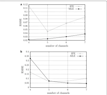
Influence of the number of channels
Figure 6 shows the results of the experiments which evaluated the influence of the num-ber of channels on CV estimation, considering a force level of 20 % of the MVC. For 16 dB SNR signals (Fig. 6b), both, MLE and IPE methods have similar behavior, with RMSE decreasing while the number channels used to CV estimation increases. For noise free signals (Fig. 6a), both algorithms presents the RMSE increasing with channel (except for
0.02 0.03 0.04 0.05 0.06 0.07 0.08 0.09 0.1 0.11 0.12
4 5 6 7
number of channels
RMS
E
IPE MLE
0 0.05 0.1 0.15 0.2 0.25 0.3 0.35 0.4
4 5 6 7
number of channels
RMS
E
IPE MLE a
b
Fig. 6 Evaluation of the influence of the number of channels on CV estimation in the MLE and IPE methods,
5 channels in MLE method). In all cases, it is evident that the use of 5 or more channels is recommended to avoid RMSE higher than the high-goodness threshold.
CV experiments using real biceps brachii S‑EMG signals
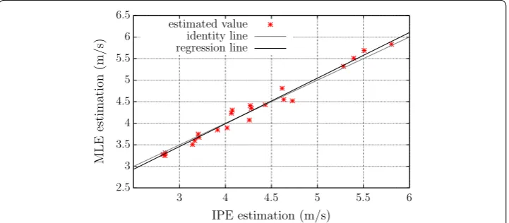
Figure 7 shows a scatter plot comparing MLE- and IPE-measured CV values from 22 S-EMG signals measured on the biceps brachii muscle of healthy volunteers, during 10-s isometric contractions, at 20 % of the MVC. Five more signals were evaluated with both algorithm but due to outlier results on the MLE method, this number was reduced to 22 and the outliers were evaluated separately. The green dashed line is the regression line and the red dashed line is the identity line. The results show a strong linear correla-tion between the two algorithms (correlacorrela-tion coefficient was 0.99, p<0.01), which
indi-cates good agreement. The slope of the regression line was 1.06, and its linear coefficient was −0.24 m/s. If we include the outliers, the correlation coefficient drops to 0.77. In all outlier cases, the MLE method results in non-physiological CV values—6.3, 7.6, 8.0, 8.9 and 9.4 m/s, whereas the IPE method estimated values were respectively 4.5, 4.3, 5.6, 7.0 and 5.0 m/s. These IPE estimates are closer to physiological values, which suggest lower errors, but we don’t know the real mean CV for these signals. In all cases of outliers we noted a high number of MUAP superpositions, which may be the reason for the MLE error. These results suggest that the IPE method is less sensitive to MUAP superposi-tions than MLE.
Discussion
The experiments using simulated signals showed that it is possible to robustly estimate the average CV of multichannel S-EMG signals using image processing techniques. When the CV was 3, 4 or 5 m/s, and the SNR was high (≥16 dB), the proposed IPE algorithm was as precise and accurate as the MLE method proposed by Farina et al. [12]. When the SNR was low (=12 dB), the MLE method performed not as well as the IPE
method, but generally provided acceptable results (RMSE <0.5 m/s, which still allows detecting variations of the average CV [12]). The performance of the IPE algorithm
2.5 3 3.5 4 4.5 5 5.5 6 6.5
3 4 4.5 5 5.5 6 IPE estimation (m/s)
MLE
estimation
(m/s)
estimated value identity line regression line
Fig. 7 Scatter plot comparing MLE- and IPE-measured CV values from 22 S-EMG signals measured on the
degrades when the SNR is low, because false conduction lines due to noise remain even after morphological transformation. However, IPE algorithm performed better than MLE for these SNR.
It is important to note, however, that signals with SNR lower than 20 dB are not com-monly used. Noise levels in adequately-performed S-EMG experiments are typically on the order of 2–10 µVrms, while typical amplitude values for S-EMG signals are on the order of 4–5 mVpp [37].
The fact that IPE method performed better than the MLE method may be because the IPE algorithm does not rely on an initial guess for the CV. The issue of CV initializa-tion can be critical when using the MLE method, especially when the SNR is low. When the true CV is considerably higher than the user-defined initial guess, the MLE method tends to provide incorrect CV estimates. Similarly, if the wrong direction of MUAP propagation is assumed, the MLE algorithm tends to provide highly imprecise estimates. These issues with the MLE algorithm are due to local minima problems associated with the Newton–Raphson method. The proposed IPE method does not use iterative optimi-zation methods, therefore it is not susceptible to this type of error, and does not require any a priori information about the direction of MUAP propagation.
For all the simulated signals we used, the channels were away from the IZs. In pre-liminary experiments with simulated signals containing one IZ, the proposed method showed better results than the MLE method. However, neither method should be used to estimate the CVs on signals containing IZs, without modification. The MLE algo-rithm, as originally proposed by Farina et al. [12], estimates the amount of delay between adjacent channels by minimizing the MSE between signals present in these two chan-nels. This delay, however, is positive for the channels positioned before the IZ and nega-tive for the channels positioned after the IZ. The MLE algorithm does not take this into consideration, and therefore is not able to accurately estimate the CV for signals containing IZs. The IPE method is potentially able to accurately estimate the CVs from conducting lines on both sides of the IZ. However, the conduction lines are generally curved near the IZ because of non-propagating potentials. Since the CV is calculated from the slope of the conduction lines, the image’s rows corresponding to channels near the IZs should be discarded before calculating the CV. An automatic IZ tracking process [26, 30], followed by removal of the channels containing IZs, could be incorporated into the IPE algorithm in order to allow its use with signals containing IZs. This idea will be explored in future works.
When applied to biceps brachii signals, the proposed method showed a similar per-formance of CV with respect to the MLE method. However, the MLE method estimated non-physiological CV values for 5 real signals. For this motive these signals were dis-carded, however, IPE method was able to estimate physiological values for these cases.
Conclusion
method does not use iterative optimization methods, therefore it is not susceptible to errors associated with MUAP propagation direction or inadequate initialization param-eters, which are common with the MLE algorithm. An automatic IZ tracking process could be incorporated into the IPE algorithm in order to allow its use with signals con-taining IZs.
Image processing-based approaches may be useful in S-EMG analysis to extract differ-ent physiological parameters from multichannel S-EMG signals. A wide variety of new methods based on image analysis could be developed to estimate parameters that are difficult to assess using traditional methods, such as CV. Problems that could be inves-tigated using image processing techniques (in combination with pattern recognition methods) include: estimating the CV for individual MUs, IZ localization and tracking, EMG decomposition, and study of MU recruitment strategies.
Authors’ contributions
FA Soares conducted this research and wrote the first draft of the manuscript. JLA Carvalho co-advised this research and carried out a major revision of the manuscript. MM Andrade participated in the initial design of this study, and in signal acquisition. CJ Miosso participated in the design and analysis of CV-related experiments and carried out a major revision of the manuscript. AF da Rocha was the principal advisor of this research. All authors read and approved the final manuscript.
Author details
1 Department of Electrical Engineering, University of Brasília, Campus Darcy Ribeiro, Caixa Postal 4386, 70910-900 Bra-sília, DF, Brazil. 2 UnB Gama Faculty, University of Brasília, Area Especial de Indústria, Projeção A, Setor Leste, Gama, 72444-240 Brasília, DF, Brazil.
Acknowledgements
The authors acknowledge Prof. Roberto Merletti and Prof. Jake C. do Carmo for valuable discussions. This research was performed with the support of the following research groups of the University of Brasília: Instrumentation and Signal and Image Processing Laboratory; Digital Signal Processing Group; and Biomedical Signal Processing Laboratory. We also thank the Laboratory of Engineering of Neuromuscular System and Motor Rehabilitation (LISiN) for providing the EMG maximum likelihood estimation (MLE) tool, to which we compare our proposed method.
Compliance with ethical guidelines Competing interests
The authors declare that they have no competing interests.
Received: 29 October 2014 Accepted: 27 August 2015
References
1. Moritani T, Stegeman DF, Merletti R. Basic physiology and biophysics of the EMG signal generation. In: Merletti R, Parker PA, editors. Electromyography: physiology, engineering, and noninvasive applications,Chap. 1. Hobooken: John Wiley & Sons; 2004. pp 1–25.
2. Hakansson CH. Conduction velocity and amplitude of the action potential as related to circumference in the iso-lated fiber of frog muscle. Acta Physiol Scand. 1956;37:14–22.
3. Brody L, Pollock M, Roy S. pH induced effects on median frequency and conduction velocity of the myoelectric signal. J Appl Physiol. 1991;71:1878–85.
4. Morimoto S, Masuda T. Dependence of conduction velocity on spike interval during voluntary muscular contraction in human motor units. J Appl Physiol. 1984;53:191–5.
5. Merletti R, De Luca CJ. New techniques in surface electromyography. In: Desnedt JE, editor. Computer aided electro-myography and expert systems. Clarendon: Elsevier; 1989.
6. Andreassen S, Arendt-Nielsen L. Muscle fiber conduction velocity in motor units of the human anterior tibial mus-cle: a new size principle parameter. J Physiol. 1987;391:561–71.
7. Arendt-Nielsen L, Mills KR. The relationship between mean power frequency of the EMG spectrum and muscle fibre conduction velocity. Electroencephalogr Clin Neurophysiol. 1985;60:130–4.
8. De Luca CJ. Physiology and mathematics of myoelectric signals. IEEE Trans Biomed Eng. 1979;26:313–25.
9. Merletti R, Knaflitz M, De Luca CJ. Myoelectric manifestations of fatigue in voluntary and electrically elicited contrac-tions. J Appl Physiol. 1990;69:1810–20.
11. van der Hoeven JH, Zwarts MJ, van Weerden TW. Muscle fiber conduction velocity in amyotrophic lateral sclerosis and traumatic lesions of the plexus brachialis. Electroencephalogr Clin Neurophysiol. 1993;89:304–10.
12. Farina D, Muhammad W, Fortunato E, Meste O, Merletti R, Rix H. Estimation of single motor unit conduction velocity from surface electromyogram signals detected with linear electrode arrays. Med Biol Eng Comput. 2001;39:225–36. 13. Broman H, Bilotto G, Luca CJD. Myoelectric signal conduction velocity and spectral parameters: influence of force
and time. J Appl Physiol. 1985;58:1428–37.
14. Lindstrom L, Magnusson R. Interpretation of myoelectric power spectra: a model and its applications. Proc IEEE. 1977;65:392–9.
15. McGill K, Dorfman L. High resolution alignment of sampled waveforms. IEEE Trans Biomed Eng BME. 1984;31:462–70.
16. Naeije M, Zorn H. Estimation of action potential conduction velocity in human skeletal muscles using the surface EMG cross-correlation technique. Electromyogr Clin Neurophysiol. 1983;23:73–85.
17. Hunter LW, Kearney RE, Jones LA. Estimation of the conduction velocity of muscle action potentials using phase and impulse response function techniques. Med Biol Eng Comput. 1987;25:121–6.
18. Arendt-Nielsen L, Zwarts M. Measurement of muscle fiber conduction velocity in humans: techniques and applica-tions. J Clin Neurophysiol. 1989;6:73–190.
19. Conte LRL, Merletti R. Advmaces in processing of surface myoelectric signals: part 2. Med Biol Eng Comput. 1995;33:373–84.
20. Merletti R, Lo Conte LR. Advances in processing of surface myoelectric signals: parts 1 and 2. Med Biol Eng Comput. 1995;33:362–84.
21. Fortunato E. Methods for estimating muscle fiber conduction velocity distribution. PhD thesis, Torino, Italy: Dept. Electron, Politecnico di Torino, 1998.
22. Farina D, Merletti R. Comparison of algorithms for estimation of EMG variables during voluntary isometric contrac-tions. J Electromyogr Kinesiol. 2000;10:337–49.
23. Farina D, Merletti R. Methods for estimating muscle fibre conduction velocity from surface electromyographic signals. Med Biol Eng Comput. 2004;42:432–45.
24. Grönlund C. Ostlund, Roeleveld, Karlsson: simultaneous estimation of muscle fibre conduction velocity and muscle fibre orientation using 2D multichannel surface electromyogram. Med Biol Eng Comput. 2005;43:63–70.
25. Farina D, Fortunato E, Merletti R. Noninvasive estimation of motor unit conduction velocity distribution using linear electrode arrays. IEEE Tr. 2000;47:380–8.
26. Soares, F.A., Andrade, M.M., da Rocha, A.F., Merletti, R.: Automatic tracking of innervation zones using image process-ing methods. In: ISSNIP Biosignals and Biorobotics Conference 2010, Vitoria-ES, Brazil, IEEE Computer Society, 2010, pp 214–218
27. Gonzalez RC, Woods RE. Digital Image Processing. Upper Saddle River: Pearson Education Inc; 2008.
28. Soares FA, Salomoni S, da Rocha AF. S-EMG conduction velocity estimation using image processing techniques. In: Proceedings of ISEK 2010, Alborg 2010.
29. Soares FA, Carvalho JLA, Miosso CJ, da Rocha AF. Estimation of conduction velocity means and variances associated to S-EMG signals based on image processing techniques [in portuguese]. In: Annals of the XXIII Brazilian Biomedical Engineering Conference, 2012. pp 2111–2115.
30. Soares FA, Zaghetto A, de Carvalho JLA, da Rocha AF. Tracking of multiple innervation zones in multichannel S-EMG signals using image processing techniques [in portuguese]. In: Annals of the XXIII Brazilian Biomedical Engineering Conference, 2012. pp 2116–2120
31. Ullah K, Afsharipour B, Merletti R. EMG topographic image enhancement using multi scale filtering. XIII Mediter-ranean Conference on Medical and Biological Engineering and Computing 2013, vol. 41., IFMBE ProceedingsSevilla, Spain: Springer; 2014. p 674–7.
32. Rivero-Moreno CJ, Bres S, Eglin V. Hermite filter-based texture analysis with application to handwriting document indexing. In: Image Analysis and Recognition, Springer, Berlin, Heidelberg 2005. pp 737–745.
33. Rodriguez I, Gila AL, Malanda, Gurtubay IG, Mallor F, Gomez S, Rodriguez J, Navallas J. Motor unit action potential duration, I: variability of manual and automatic measurements. J Clin Neurophysiol. 2007;24:52–8.
34. Farina D, Merletti R. A novel approach for precise simulation of the EMG signal detected by surface electrodes. IEEE Trans Biomed Eng. 2001;4:637–46.
35. Merletti R, Rainoldi A, Farina D. Myoelectric manifestations of muscle fatigue. In: Merletti R, Parker PA, editors. Electro-myography: physiology, engineering, and noninvasive applications, Chap. 9. Hobooken: John Wiley & Sons; 2004. pp 233–58.
36. Soares FA, Salomoni SE, Veneziano WH, de Carvalho JLA, Nascimento FAO, Pires KF, da Rocha AF. On the behavior of surface electromyographic variables during the menstrual cycle. Phisiol Meas. 2011;32:543–57.