R E S E A R C H A R T I C L E
Open Access
Estimating correlation between multivariate
longitudinal data in the presence of
heterogeneity
Feng Gao
1,2*, J. Philip Miller
2, Chengjie Xiong
2, Jingqin Luo
1,2, Julia A. Beiser
3, Ling Chen
2and Mae O. Gordon
2,3Abstract
Background:Estimating correlation coefficients among outcomes is one of the most important analytical tasks in epidemiological and clinical research. Availability of multivariate longitudinal data presents a unique opportunity to assess joint evolution of outcomes over time. Bivariate linear mixed model (BLMM) provides a versatile tool with regard to assessing correlation. However, BLMMs often assume that all individuals are drawn from a single homogenous population where the individual trajectories are distributed smoothly around population average.
Methods:Using longitudinal mean deviation (MD) and visual acuity (VA) from the Ocular Hypertension Treatment Study (OHTS), we demonstrated strategies to better understand the correlation between multivariate longitudinal data in the presence of potential heterogeneity. Conditional correlation (i.e., marginal correlation given random effects) was calculated to describe how the association between longitudinal outcomes evolved over time within specific subpopulation. The impact of heterogeneity on correlation was also assessed by simulated data.
Results:There was a significant positive correlation in both random intercepts (ρ= 0.278, 95% CI: 0.121–0.420) and random slopes (ρ= 0.579, 95% CI: 0.349–0.810) between longitudinal MD and VA, and the strength of correlation constantly increased over time. However, conditional correlation and simulation studies revealed that the correlation was induced primarily by participants with rapid deteriorating MD who only accounted for a small fraction of total samples.
Conclusion:Conditional correlation given random effects provides a robust estimate to describe the correlation between multivariate longitudinal data in the presence of unobserved heterogeneity (NCT00000125).
Keywords:Bivariate linear mixed model (BLMM), Multivariate longitudinal data, Correlation, Heterogeneity
Background
Estimating the correlation coefficients between outcome variables is one of the most important analytical tasks in epidemiological and clinical research. When independent observations are available for each outcome variable, Pearson’s correlation coefficients are often used. In many epidemiological and clinical studies, however, the same individuals are also followed repeatedly over time for a series of measurements with regarding to the collection of outcome variables. Such multivariate longitudinal data provide a unique opportunity to study the joint evolution
of these outcomes over time. A simple Pearson’s correl-ation coefficient is no longer applicable for assessing cor-relation because a multivariate longitudinal model has to account for two types of correlations simultaneously, namely the serial correlation between observations at different time points within a subjects and the cross correlation between observations on different outcome variables at each time point [1].
During the last few decades, many statistical models have been proposed in statistical literature for the analysis of multivariate longitudinal data and the most popular one is the joint mixed model which links separate linear mixed models by allowing their model-specific random effects to be correlated [2]. The advantages of this approach include well-established theory [1], efficiency gains [3], and com-mercially available software packages for model fit [4, 5].
* Correspondence:[email protected] 1
Department of Surgery, Division of Public Health Sciences, Washington University School of Medicine, 660 S. Euclid Ave., St. Louis, MO 63110, USA 2Division of Biostatistics, Washington University School of Medicine, 660 S. Euclid Ave., St. Louis, MO 63110, USA
Full list of author information is available at the end of the article
More importantly, a joint random-effect model allows assessing correlation between different outcomes. It can provide a succinct summary for not only how the evolution of one outcome variable is correlated to the evolution of another outcome (“association of evolution”), but also how the correlation between outcomes changes over time (“evolution of association”) [6].
Various extensions have been made in recent years in joint mixed models for a wide range of research fields [2, 7]. A typical joint mixed model often consists very few (usually 2 or 3) continuous outcome variables, takes a linear parametric functional form over time, holds a multivariate normality distribution for the vector of ran-dom effects, and assumes that the outcome variables are mutually independent given random effects. Fieuws and Verbeke [6] relaxed the conditional independence as-sumption by allowing the error components of the out-comes to be correlated. Gueorguieva and Sanacora [3] developed a joint mixed model to incorporate different types of longitudinal outcomes and analyzed repeated measurements on ordinal and continuous variables meas-uring the same underlying disease severity over time. Fieuws and Verbeke [8] took a pairwise fitting approach to construct the variance-covariance matrix for the joint distribution of random effects and assessed the hearing threshold profiles (22 outcomes) in a nature aging study. Putter et al. [9] proposed a latent class joint model (e.g., assuming the vector of random effects following a multi-nomial rather than normal distribution) to identify lung cancer patients with distinct patterns regarding their evolvement of denial over time and to assess the as-sociation between denial patterns and the trajectories of other physical and emotional longitudinal measure-ments. Recently Luo et al. [10] extended the model to non-longitudinal setting and proposed a bivariate lin-ear mixed model to estimate correlation coefficients in cross-sectional data from a family-type clustered design. For other approaches in the analysis of multi-variate longitudinal data as well as for more details in recent development, see the comprehensive reviews by McCulloch [7], Bandyopadhyay et al. [11], Verbeke et al. [2] and the references therein.
Almost all of the aforementioned joint mixed models (except Putter et al. [9]) also assume that subjects are drawn from a single homogenous population and that the individual trajectories are smoothly distributed around the population average. In this article, we intended to address the issue when such a one-size-fit-all assumption is violated, using participants with newly diagnosed primary open angle glaucoma (POAG) from the Ocular Hypertension Treatment Study (OHTS). POAG is a chronic progressive optic neuropathy and the rate of vision deterioration can vary substantially from patient to patient. For example, a natural history
study on a cohort of patients newly diagnosed with glaucoma found out that the mean deviation (MD) index, a global summary measure for visual field test, in some patients can deteriorate at an alarming rate of 10 dB (dB) per year, while in others the MD virtually did not change in 6 years without any treatment [12]. It is therefore important to take potential heterogeneity into consideration when correlation is assessed.
In this article, we demonstrated strategies to assess the correlation between multivariate longitudinal data in the presence of potential heterogeneity. Specifically, bivariate linear mixed model (BLMM) was fitted to assess both the “association of evolution” (i.e., correlation between random effects) and“evolution of association” (i.e., mar-ginal correlation over time), and then conditional correl-ation (i.e., marginal correlcorrel-ation given random effects) was calculated to describe how the association between longitudinal outcomes evolved over time within a“true” but unobserved subset of individuals. The disease hetero-geneity was also approximated by subgroups (latent clas-ses) from latent class analysis (LCA) where population variability is captured by differences across subgroups in the shape and level of their trajectories [13]. These sub-groups were incorporated into BLMMs to further under-stand the impact of heterogeneity on correlation. Our method was similar to the latent class joint model by Putter et al. [9] except that our primary goal focused on correlations rather than trajectories. The remainder of this paper was structured as follows. Section 2 described the OHTS data in more detail. Section 3 specified the bivari-ate linear mixed model (BLMM) model to assess correl-ation among multivariate longitudinal data. The method was applied to data from OHTS in Section 4 and a simple simulation study was also performed to assess the impact of heterogeneity on correlation in Section 5. Finally, we concluded with a discussion in Section 6.
Study cohort: Ocular hypertension treatment study (OHTS)
Between 1994 and 2009, the OHTS enrolled 1636 partic-ipants with ocular hypertension but with no evidence of glaucomatous damage and randomized to either obser-vation or treatment with ocular hypotensive medication. The participants were followed for a median of 13 years and the disease progression was monitored regularly every 6 months. In OHTS, 362 eyes from 279 partici-pants developed POAG during study and constituted the largest cohort of POAG with known date of diagnosis, with a median pre-diagnosis follow-up of 8 years and median post-diagnosis follow-up of 4.8 years. The design and methods of the OHTS have been described in detail elsewhere [14].
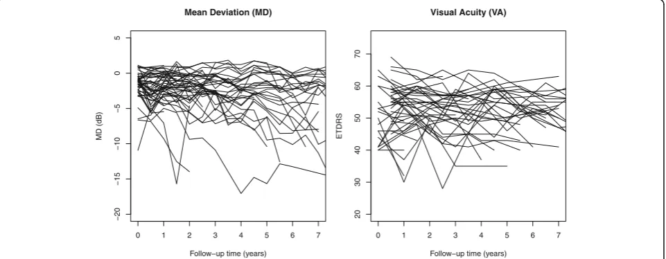
diseases, multiple longitudinal outcomes were collected in OHTS to fully explore the multidimensional impairment caused by POAG. Our analysis restricted to 2 longitudinal outcomes, namely mean deviation (MD) and clinical vis-ual acuity (VA). MD is a global index from Humphrey 30–2 visual field (VF) tests and reflectsfunctional damage. VA is measured by the standard ETDRS acuity testing (ETDRS ranged 0 to 110, with the conventional 20/20 vision corresponding to ETDRS score of 100) and a low ETDRS score indicates a poor visual ability. MD was mea-sured every 6 months while VA was meamea-sured annually. This study has been approved by Washington University Institutional Review Board. Our analysis cohort consisted the first eye of 269 OHTS participants who developed POAG and had at least 2 post-diagnosis measurements in both MD and VA. To reduce the potential influence of cases with greater attrition rates, we excluded all the mea-sures taken 7.5 years after diagnosis and ended up with at least 30 observations in each outcome at any given time points. Figure 1 showed the raw data of 50 randomly selected participants and there was a considerable variabil-ity in the trajectories for both MD and VA. Besides these two longitudinal outcomes, following demographic and clinical characteristics were also included in the data: age at diagnosis (years), gender, race (African American vs. Others), randomization groups (Observation vs. Treat-ment), intraocular pressure (IOP, mmHg), central corneal thickness (CCT,μm), and horizontal cup/disc ratio (HCD).
Methods
Since MD is arguably the most important index for monitoring POAG progression in clinical practice, in this article we focused on the heterogeneity of this pivotal variable and its impact on the correlation between MD and VA.
Bivariate linear mixed model (BLMM) between MD and VA
Let Y1i(t) and Y2i(t) denote the MD and VA for ith par-ticipant at time t, Zi= {AGE, Gender, Race, Observation group, CCT, IOP, HCD} be the vector of baseline covari-ates of ith participant, then each outcome can be described by a linear mixed model,
Y1ið Þ ¼t ZiαZþðα0þα0iÞ þðα1þα1iÞtijþε1ið Þt ;
Y2ið Þ ¼t ZiβZþ β0þβ0i
þ β1þβ1i
tijþε2ið Þt :
Where {α0,β0} is the vector of intercepts, {α1,β1}is the vector of slopes during post-diagnosis period, while {αZ,βZ} is the vector of fixed effects for all other co-variates at diagnosis. {a0i,a1i}and{b0i,b1i,b2i}represent random intercept and slope for longitudinal MD and VA respectively, and the BLMM is constructed by linking the two outcomes via a joint distribution of the random effects,
"
a0ib0i
a1i
b1i
#
eNð0;ΣÞ; Σ¼
"
σ2
a0 σa0b0 σa0a1 σa0b1
σ2
b0 σa1b0 σb0b1
σ2
a1 σa1b1
σ2
b1
#
The error terms assume following bivariate normal distribution and independent of random effects,
"
ε1i
ε2i
#
eN 00 ;
σ2
1 0
0 σ22
" #!
:
Estimated correlations between longitudinal MD and VA
Once the BLMM has been fitted and the variance-covariance matrix is obtained, the correlation between
0 1 2 3 4 5 6 7
−20
−15
−10
−5
0
5
Mean Deviation (MD)
Follow−up time (years)
MD (dB)
0 1 2 3 4 5 6 7
20
30
40
50
60
70
Visual Acuity (VA)
Follow−up time (years)
ETDRS
MD and VA can be calculated analytically and following 3 different types of correlations are estimated in this paper.
Association of evolution (correlation between random effects)
The correlation between random effects (intercepts and post-diagnosis slopes) summarizes how the evolution of MD is associated with the evolution of VA [6],
ρintercept¼
σa0b0
ffiffiffiffiffiffiffi σ2 a0 q ffiffiffiffiffiffiffi σ2 b0
q ; and ρslope¼ ffiffiffiffiffiffiffiσa1b1
σ2 a1 q ffiffiffiffiffiffiffi σ2 b1 q :
Evolution of association (marginal correlation)
The marginal correlation during post-diagnosis period allows answering the question how the association between MD and VA evolves over time [6],
ρmarginalð Þ ¼t
σa0b0þtσa0b1þtσa1b0þt
2σ a1b1
ffiffiffiffiffiffiffiffiffiffiffiffiffiffiffiffiffiffiffiffiffiffiffiffiffiffiffiffiffiffiffiffiffiffiffiffiffiffiffiffiffiffiffiffiffiffiffiffiffiffiffiffi
σ2
a0þ2tσa0a1þt2σ2a1þσ
2 1
q ffiffiffiffiffiffiffiffiffiffiffiffiffiffiffiffiffiffiffiffiffiffiffiffiffiffiffiffiffiffiffiffiffiffiffiffiffiffiffiffiffiffiffiffiffiffiffiffiffiffiffiffi
σ2
b0þ2tσb0b1þt2σ2b1þσ
2 2
q :
Conditional correlation (marginal correlation given random effects)
The conditional marginal correlation given specific ran-dom effects allows us to assess how the association be-tween MD and VA evolves over time within certain clinically relevant subgroups. Since a majority of POAG participants tends to have a relatively stable vision func-tion for a long period over time after initial diagnosis, the correlation between MD and VA in the participants with stable vision would provide a useful tool to assess the impact of heterogeneity. Let γ0i=ZiαZ+α0+a0iand
γ1i=α1+a1i denote the random intercept and slope of MD for ith participant, let Y1i(t) and Y2i(t) denote MD and VA for ithparticipant at time t, then the joint distri-bution of {Y1i(t), Y2i(t), γ0i, γ1i} at given time t also follows a normal distribution,
Y1ið Þt
Y2ið Þt
γ0i γ1i 0 B B @ 1 C C AeN
ZiαZþα0þα1t
ZiβZþβ0þβ1t
ZiαZþα0
α1 0 B B @ 1 C C A;
ν11ð Þt ν12ð Þt ν13ð Þt ν14ð Þt
ν22ð Þt ν23ð Þt ν24ð Þt
ν33 ν34
ν44 0 B B @ 1 C C A 0 B B @ 1 C C A, with
υ11ð Þ ¼t σ2a0þt 2σ2
a1þ2tσa0a1þσ 2 1;
υ22ð Þ ¼t σ2b0þt 2σ2
b1þ2tσb0b1þσ 2 2;
υ12ð Þ ¼t σa0b0þtσa0b1þtσa1b0þt 2σ
a1b1;
υ13ð Þ ¼t σ2a0þtσa0a1; υ14ð Þ ¼t σa0a1þtσ 2
a1;
υ23ð Þ ¼t σa0b0þtσa0b1; υ24ð Þ ¼t σa1b0þtσa1b1;
υ33¼σ2a0; υ34¼σa0a1; and υ44 ¼σ 2
a1:
Once the bivariate linear mixed model has been fitted and its variance-covariance matrix is obtained, the joint
distribution of {Y1i(t), Y2i(t), γ0i, γ1i} at given time t can be obtained by plugging in the estimated parameters. The conditional correlation at a given time t is denoted asρ(Y1i(t), Y2i(t)|γ0i > c1,γ1i> c2), where c1and c2 rep-resent clinical relevant thresholds for the intercept and slope of MD respectively. In the clinical practice of POAG management, an MD level of -5 dB or above marks a mild damage and MD < −5 dB is deemed as moderate/advanced damage. An MD slope of−1 dB/year is often regarded as clinically significant deterioration. Since this paper only includes participants with newly diagnosed POAG, it is believed that a change of
−0.5 dB/year is also worthy close attention [15]. We therefore choose c1=−5 dB and c2=−0.5 dB/years throughout the remainder of this paper. Once the pa-rameters from bivariate mixed models have been deter-mined, the conditional correlation ρ(Y1i(t), Y2i(t)|
γ0i > c1, γ1i > c2) can be estimated using parametric bootstrap resampling method with the following 4 steps.
1. At a given time t, a random sample ofN= 269 subjects is generated from the above multivariate normal distributions, N(μi(t),∑(t)), withi= 1, 2,…, 269. Each dataset includes 4 variables, MD (Y1i), VA (Y2i), intercept of MD (γ0i), and slope of MD (γ1i). 2. Pearson’s correlation coefficient between MD and
VA is calculated among these subjects who satisfy the conditions (i.e., with MD at diagnosis >−5 dB and slope of MD >−0.5 dB/year).
3. The above 2 steps are repeated 10,000 times to obtain the average conditional correlation at time t. The 95% confidence interval is also estimated as the 2.5 and 97.5 percentiles of the resultant correlations. 4. The above steps are repeated over different time
points to describe the change of marginal correlations over time.
The assumption of independent errors in the above model could be relaxed if necessary [6]. In the case of
correlated errors,
ε1i
ε2i
!
∼N 0
0 ;
σ2 1 σ12
σ12 σ22
!!
, the
formula for correlations between random effects remain unchanged, but the marginal correlation over time is cal-culated as follows and the term v12(t) for conditional marginal correlation also needs to be updated accordingly,
ρmarginalð Þ ¼t σa0b0
þtσa0b1þtσa1b0þt2σa1b1þσ12
ffiffiffiffiffiffiffiffiffiffiffiffiffiffiffiffiffiffiffiffiffiffiffiffiffiffiffiffiffiffiffiffiffiffi
σ2
a0þ2tσa0a1þt2σ2a1þσ 2 1
p ffiffiffiffiffiffiffiffiffiffiffiffiffiffiffiffiffiffiffiffiffiffiffiffiffiffiffiffiffiffiffiffiffiffi
σ2
b0þ2tσb0b1þt2σ 2 b1þσ
2 2
p ;
and υ12ð Þ ¼t σa0b0þtσa0b2þtσa2b0þt 2σ
parametric bootstrap samples, while the 95% CIs of other correlations were obtained from 500 empirical bootstrap samples using participants as resampling units. All the BLMMs were fitted using the MIXED procedure in SAS statistical package 9.4 (SAS Institutes, Cary, NC).
Results
Application to ocular hypertension treatment study (OHTS)
Table 1 showed the summary statistics for baseline demographic characteristics, the estimated regression coefficients, and the estimated parameters of the variance-covariance from univariate mixed model to each outcome. Among these baseline covariates, age was significantly associated with both outcomes and these elderly participants had poor outcomes. Those partici-pants with higher intraocular pressure (IOP) at diagnosis or with lower central corneal thickness (CCT) had sig-nificantly worse MD. Participants self-identified as African-American also tended to be worse in both out-comes though the difference was only significant in VA. Note that all the continuous variables (Age, CCT, IOP, and HCD) were standardized to have mean 0 and
variance 1 in all the models throughout this paper and hence the regression coefficients actually represented the effect per 1-SD change.
Primary analysis for the correlation between longitudinal MD and VA
Two bivariate linear mixed models (BLMM) were fitted to describe the relationship between MD and VA, one assuming correlated error terms and the other with in-dependent errors. The likelihood ratio test showed that the model with independent errors would provide an ad-equate fit (X2= 2.9, df = 1, p= 0.09). Hence, the BLMM with independent error terms was selected as the final model. The estimated fixed and random effects from this BLMM were presented in Table 1. The results showed that the univariate and bivariate mixed models produced very close estimates, especially the fixed effects. Follow-ing Fieuws et al. [6], the correlation between longitudinal MD and VA was summarized in terms of the association between subject-specific evolutions (as measured by ran-dom intercepts and slopes) as well as the evolution of association (as measured by marginal correlation over time). Table 2 presented the estimated correlation
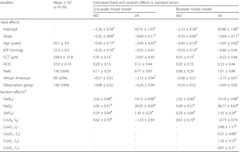
Table 1Summary statistics of baseline covariates, the estimated regression coefficients, and the estimated parameters of variance (Var) and covariance (Cov) from the univariate and bivariate mixed models for longitudinal mean deviation (MD) and visual acuity (VA)
Variables Mean ± SD
or N (%)
Estimated fixed and random effects ± standard errors
Univariate mixed model Bivariate mixed model
MD VA MD VA
Fixed effects:
Intercept - −2.26 ± 0.34# 50.75 ± 1.03# −2.23 ± 0.34# 50.88 ± 1.00#
Slope - −0.35 ± 0.04# −0.60 ± 0.11# −0.35 ± 0.04# −0.69 ± 0.11#
Age (years) 65.7 ± 9.5 −0.49 ± 0.15# −3.45 ± 0.43# −0.43 ± 0.14# −3.07 ± 0.42#
IOP (mmHg) 22.3 ± 6.2 −0.55 ± 0.16# −0.55 ± 0.47 −0.55 ± 0.16# −0.40 ± 0.45
CCT (μm) 558.4 ± 37.8 0.35 ± 0.15* −0.07 ± 0.45 0.35 ± 0.15* −0.22 ± 0.44
HCD 0.53 ± 0.19 0.20 ± 0.15 0.12 ± 0.44 0.20 ± 0.15 0.12 ± 0.44
Male 150 (56%) 0.11 ± 0.29 0.77 ± 0.87 0.06 ± 0.29 1.01 ± 0.84
African American 89 (33%) −0.57 ± 0.31 −2.13 ± 0.94* −0.58 ± 0.31 −2.15 ± 0.91*
Observation group 158 (59%) −0.08 ± 0.32 −0.26 ± 0.94 −0.10 ± 0.32 −0.69 ± 0.92
Random effects:&
Var(Ek) 2.03 ± 0.06# 19.15 ± 0.96# 2.02 ± 0.06# 19.19 ± 0.96#
Var(Ik) 5.05 ± 0.51# 39.25 ± 4.69# 5.09 ± 0.51# 38.77 ± 4.63#
Var(Sk) 0.29 ± 0.04# 1.35 ± 0.25# 0.29 ± 0.04# 1.35 ± 0.24#
Cov(Ik, Sk) 0.62 ± 0.10# −1.23 ± 0.83 0.63 ± 0.10# −0.73 ± 0.79
Cov(I1, I2) - - - 3.88 ± 1.17#
Cov(S1, S2) - - - 0.37 ± 0.08#
Cov(I1, S2) - - - 1.16 ± 0.27#
Cov(I2, S1) - - - 0.67 ± 0.31*
IOPintraocular pressure,CCTcentral corneal thickness,HCDhorizontal cup-to-disc ratio
&
Ek, Ik, Sk: error term, random intercept, and random slope for MD (k = 1) and VA (k = 2) *
coefficients for random intercepts and slopes and their 95% confidence intervals (CI). There was a significant positive correlation in both random intercepts (ρ= 0.278, 95% CI: 0.121–0.420) and random slopes (ρ= 0.579, 95% CI: 0.349–0.810).
Figure 2 plotted the marginal correlations (solid lines) and the corresponding 95% confidence intervals (broken lines). Pearson correlation coefficient estimated at each time point was also used as a naïve approximation to the marginal correlation over time. In general, the marginal correlation at diagnosis (time 0) approximated the ation between random intercepts, and the marginal correl-ation converged to the correlcorrel-ation between random slopes as the time departures from 0 [6]. As comparing to the unconditional correlation, the conditional correlation in participants with stable vision function (i.e., given MD at diagnosis above−5 dB and MD slope >−0.5 dB/year) re-duced substantially, indicating that the observed correl-ation between MD and VA was mainly induced by these participants with more deteriorating conditions. Figure 2 also revealed a considerable variation from time to time in the pointwise Pearson correlation, even after we had im-posed the restriction so that the analysis cohort contained at least 30 participants at any given time point.
Sensitivity analyses
Several sensitivity analyses were further performed to better understand the impact of heterogeneity on asses-sing correlations. The disease heterogeneity was approxi-mated by 4 subpopulations from a previous study using the same OHTS dataset [16]. Briefly, the trajectories of MD and pattern standard deviation (PSD, another global index of visual field tests) were summarized by a non-parametric functional principal component (FPC) analysis [17], and a latent class analysis (LCA) was performed to the first FPC scores to identify subgroups (latent classes) of individuals with distinct patterns of MD and PSD trajectories. Unlike a linear mixed model that described the individual trajectories by assuming them as random effects following a continuous distribu-tion, the LCA approach used latent classes (unobserved trajectory groups) as an approximation of the unknown distribution. In the other words, the latent classes could be thought of as longitudinal strata where population
variability was captured by differences across groups in the shape and level of their trajectories [13].
Table 4 summarized the class-specific intercepts and slopes for MD and VA respectively, after adjusting the baseline covariates. It showed that the profiles in the 4th -class were substantially different from the other -classes. Since MD < −5 dB marks a moderate/advanced vision damage and a deteriorating rate of−0.5 dB/year is deemed clinically significant in newly diagnosed POAG [15], we therefore labeled Classes 1 to 4 as “Stable, High MD”,
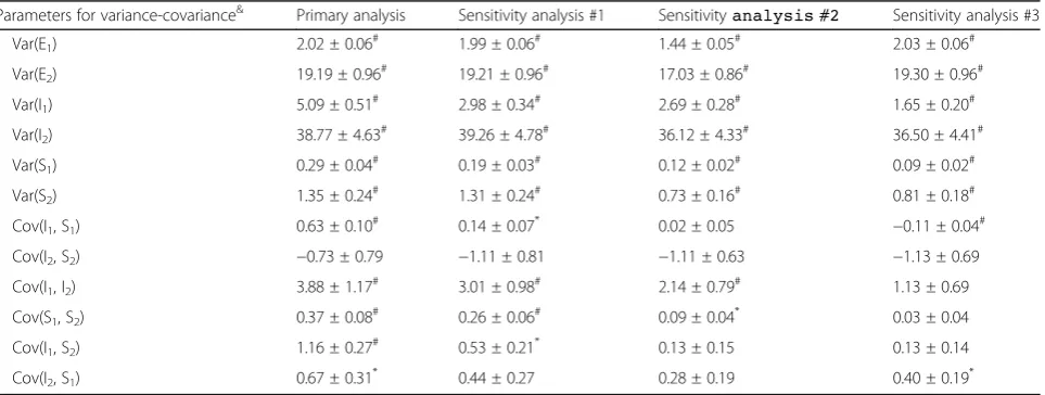
“Stable, Low MD”,“Progression”, and“Rapid Progression”, respectively. Following 3 BLMMs were fitted as sensitivity analyses. The average correlation coefficients between ran-dom effects and their 95% confidence intervals from each model were presented in Table 2. The estimated parame-ters of variance and covariance from each model were also presented in Table 3.
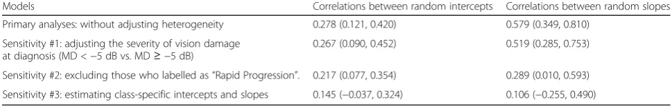
Sensitivity Analysis #1:adjusting the severity of
vision damage at diagnosis. The first BLMM incorporated an indicator for moderate/advanced glaucoma (MD <−5 dB) into the primary analysis. The model lead to similar estimates as these from primary analysis, though the strength of estimated correlation in the sensitivity analysis decreased slightly towards null.
Sensitivity Analysis #2:excluding those participants
who are labeled as“Rapid Progression”. The 2nd BLMM was fitted after excluding these 16 participants who were labeled as“Rapid Progression”. Although these participants only accounted for 6% of total sample size, excluding them lead to a substantial decrease in the estimated correlation, especially between random slopes.
Sensitivity Analysis #3:full adjustment of
heterogeneity.The 3rdsensitivity analysis fit a BLMM including both specific intercepts and class-specific slopes. The results showed that none of the correlation was significantly different from 0, indi-cating a conditional independence between MD and VA given the heterogeneity of MD trajectory.
In summary, the results revealed that the assumption of homogeneous population in BLMM is important for
Table 2Estimated correlation coefficients and their 95% confidence intervals in the random intercepts and random slopes, from the primary analysis and three sensitivity analyses using bivariate linear mixed models
Models Correlations between random intercepts Correlations between random slopes
Primary analyses: without adjusting heterogeneity 0.278 (0.121, 0.420) 0.579 (0.349, 0.810)
Sensitivity #1: adjusting the severity of vision damage at diagnosis (MD <−5 dB vs. MD≥ −5 dB)
0.267 (0.090, 0.452) 0.519 (0.285, 0.753)
Sensitivity #2: excluding those who labelled as“Rapid Progression”. 0.217 (0.077, 0.354) 0.289 (0.010, 0.593)
assessing correlation between multivariate longitudinal data. As illustrated in different sensitivity analyses, the es-timated correlations could be substantially distorted in the presence of unobserved heterogeneity. In general, the ad-justment of heterogeneity tended to reduce the strength of correlations, but all the estimates had a relatively wide range of 95% confidence interval, especially between ran-dom slopes. In such a real-world data analysis, however, we do not know the“true”population parameters and the estimates could be influenced by sampling errors. In the section follows, simulated data were used to quantify to
what extent the “true” correlation between longitudinal outcomes could be distorted due to heterogeneity.
Simulation study
The simulated data were a mixture of stable and progressive subjects, generated from following bivariate linear mixed models,
Yg1ið Þt
Yg2ið Þt !
¼ α
g 0þα
g 1t
βg 0þβ
g 1t
!
þ a0þa1t
b0þb1t
þ ε1ið Þt
ε2ið Þt
;
Fig. 2Estimated unconditional marginal correlation and conditional marginal correlation (given MD at diagnosis >−5 dB and slope of MD >−0.5 dB/year) in the OHTS data, wheresolid linesandbroken linesrepresented the estimated correlation and its 95% confidence intervals respectively. Pointwise Pearson correlation at each time was also presented
Table 3Estimated parameters of variance (Var) and covariance (Cov) from the primary analysis and the three sensitivity analyses using bivariate linear mixed models
Parameters for variance-covariance& Primary analysis Sensitivity analysis #1 Sensitivityanalysis #2 Sensitivity analysis #3
Var(E1) 2.02 ± 0.06# 1.99 ± 0.06# 1.44 ± 0.05# 2.03 ± 0.06#
Var(E2) 19.19 ± 0.96# 19.21 ± 0.96# 17.03 ± 0.86# 19.30 ± 0.96#
Var(I1) 5.09 ± 0.51# 2.98 ± 0.34# 2.69 ± 0.28# 1.65 ± 0.20#
Var(I2) 38.77 ± 4.63# 39.26 ± 4.78# 36.12 ± 4.33# 36.50 ± 4.41#
Var(S1) 0.29 ± 0.04# 0.19 ± 0.03# 0.12 ± 0.02# 0.09 ± 0.02#
Var(S2) 1.35 ± 0.24# 1.31 ± 0.24# 0.73 ± 0.16# 0.81 ± 0.18#
Cov(I1, S1) 0.63 ± 0.10# 0.14 ± 0.07* 0.02 ± 0.05 −0.11 ± 0.04#
Cov(I2, S2) −0.73 ± 0.79 −1.11 ± 0.81 −1.11 ± 0.63 −1.13 ± 0.69
Cov(I1, I2) 3.88 ± 1.17# 3.01 ± 0.98# 2.14 ± 0.79# 1.13 ± 0.69
Cov(S1, S2) 0.37 ± 0.08# 0.26 ± 0.06# 0.09 ± 0.04* 0.03 ± 0.04
Cov(I1, S2) 1.16 ± 0.27# 0.53 ± 0.21* 0.13 ± 0.15 0.13 ± 0.14
Cov(I2, S1) 0.67 ± 0.31* 0.44 ± 0.27 0.28 ± 0.19 0.40 ± 0.19*
&
Ek, Ik, Sk: error term, random intercept, and random slope for MD (k = 1) and VA (k = 2) *
with
a0i a1i b0i b1i 2 6 6 4
3 7 7 5 eN
0 0 0 0
2 6 6 4
3 7 7 5;Σ¼
1:65 1:13 −0:11 0:13 36:5 0:4 −1:13
0:09 0:03 0:81
2 6 6 4
3 7 7 5 0
B B @
1 C C A;
and εε1i
2i
eN 0
0 ; Σe¼
2:0 ρpffiffiffi2pffiffiffiffiffi19
ρpffiffiffi2pffiffiffiffiffi19 19:0
" #!
:
The group indicator (g = 1, 2) represented stable and progressive participants, and the fixed-effect parame-ters αg0;αg1;βg0;βg1were retrieved from the estimated parameters in the 2nd- and 4th-class (Table4), with
α1 0;α11;β
1 0;β
1 1
¼f−2;53;‐0:2;‐0:4gand
α2 0;α21;β
2 0;β
2 1
¼{‐8, 48,‐2.0,‐3.0} respectively. The parameters for random effectsΣandΣewere
obtained from BLMM in the 3rd sensitivity analysis and assumed common across the two mixture groups. t = {0, 0.5,…, 5} denoted the semi-annual measuring
times and we assumed that all individuals had exactly the same follow-up time in this simulation. Unless otherwise specified, we assumed independent
error terms (i.e.,ρ= 0) in all the simulations.
Each simulation generated 500 random samples and each sample consisted 300 subjects. In each simulation, the average correlation coefficients were calculated for both marginal correlation (unconditional and condi-tional) and correlation between random effects. Three scenarios were considered to assess to what extent the true correlation could be distorted in the presence of heterogeneity or model misspecification.
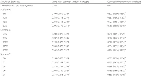
1. Scenarios A:Impact of size of heterogeneity. In the simulated data, the progressive subjects (i.e., those with g = 2) accounted for 5%, 10%, 15% and 20% of total sample size respectively. Figure3A1 showed the estimated average marginal correlation over time under different proportions of progressive cases. We saw that even the presence of a small fraction of heterogeneity could dramatically distort the estimated correlation and, as expected, greater proportion of progressive cases imposed stranger influence. In contrast, the influence of heterogeneity on the conditional correlation was much smaller, and the impact was almost ignorable in the presence of only small fraction of progressive cases (Fig.3 A2). The results also showed that the presence of heterogeneity could lead to substantial
overestimation of correlations between random effects, especially in the random slopes (Table5). 2. Scenarios B:Impact of magnitude of heterogeneity.
In each simulation, the progressive subjects accounted for only 5% of the total sample size, but the slopes in the progressive subjects varied as 50%, 75%, 125% and 150% of what were used under Scenario A. Figure3B1 showed that a higher magnitude of deterioration (like that of 4th-class in the OHTS data) could substantially distort the mar-ginal correlations over time while a lower deterior-ation (like that of 3rd-class in the OHTS data) would have little impact on the estimated correl-ation. Again, the estimated conditional correlation was relatively robust to the presence of rapid pro-gressive cases (Fig.3B2). The results also showed that higher deteriorating rate could lead to substan-tial overestimation of correlations between random slopes (Table5).
3. Scenarios C:Impact of correlation between error terms. Since a candidate BLMM in the primary analysis showed a weak correlation between error terms (ρ= 0.07) with a trend towards significance (p= 0.09), we also assessed the potential impact of independence assumption of error terms on correlation. In each simulated dataset, the progressive subjects accounted for only 5% of the total sample size and the slopes of progressive subjects were the same as those under Scenario A. The data were generated under a variety degree of correlations (ρ= 0.2, 0.4, 0.6, 0.8) between error terms, but analyzed assuming independent errors. The result showed that both the unconditional and conditional marginal correlations were rather insensitive to the degree of correlation between error terms (Fig.3C1 and C2). However, ignoring the correlation between error terms could lead to a substantial overestimation of correlations between
Table 4The trajectory profiles of longitudinal mean deviation (MD) and visual acuity (VA) across latent classes, after accounting for other baseline demographic and clinical characteristics
Parameters N (%) MD VA
Intercept:
Class1 (reference) 83 (31%) 0.08 ± 0.21 54.66 ± 0.97
Class2 117 (43%) −1.73 ± 0.23# 52.94 ± 1.08
Class3 53 (20%) −3.11 ± 0.28# 52.89 ± 1.33
Class4 16 (6%) −8.42 ± 0.45# 48.15 ± 2.17#
Slope:
Class1 (reference) 83 (31%) −0.08 ± 0.05 −0.33 ± 0.17
Class2 117 (43%) −0.15 ± 0.06 −0.35 ± 0.23
Class3 53 (20%) −0.54 ± 0.07# −0.86 ± 0.26*
Class4 16 (6%) −2.04 ± 0.13# −3.37 ± 0.47# *p< 0.05;#
random effects, especially in the random slopes. The impact was trivial when there was only a weak correlation between error terms, but became much strong in the presence of moderate/high between-error correlations (Table5).
In summary, the simulated data confirmed the relative robustness of conditional correlation to potential hetero-geneity and indicated that these participants in the Class 4 were more likely strong influential cases for assessing the correlation between longitudinal MD and VA. The sensitivity analysis excluding these 16 participants (who only account for 6% of the total samples) resulted in substantial decrease of correlation.
Discussion
In clinical trials and epidemiologic studies, it is quite common to have two or more outcomes measured re-peatedly over time. These multivariate outcomes are likely to be correlated and the statistical analysis often requires taking such associations into account. A
number of approaches for analyzing multivariate longi-tudinal data have been proposed in the statistical litera-ture, ranging from the most naïve approach of ignoring the association to the full joint model that specifies the joint distribution and correlation structure among differ-ent outcomes [1]. The choice for a specific type of model is often guided by the specific characteristics of data such as the structure of data (balance or unbalanced), the scale of outcome measures (continuous, ordinal, or binary), as well as the research questions of interest (the average evolution over time or the association structure) [11]. When the average evolution over time (fixed ef-fects) is of primary interest, for example, specification of the full joint distribution may be avoided by using a gen-eralized estimating equation (GEE) approach where as-sociation structure is treated as a nuisance, and a valid inference regarding fixed effects can still be obtained even when the within-subject associations are mis-specified. When the primary interests focus on the asso-ciation structure itself, a full joint model of outcomes is often preferred [2]. Among various joint models,
0 1 2 3 4 5
0.0
0.4
0.8
Unconditional: % of progressive cases
Time
Correlation
True (no heterogeneity) 5% cases 10% cases 15% cases 20% cases
0 1 2 3 4 5
0.0
0.4
0.8
Conditional: % of progressive cases
Time
Correlation
True (no heterogeneity) 5% cases 10% cases 15% cases 20% cases
0 1 2 3 4 5
0.0
0.4
0.8
Unconditional: deterioration rate (With 5% progressive cases)
Time
Correlation
True (no heterogeneity) 50%
75% 125% 150%
0 1 2 3 4 5
0.0
0.4
0.8
Conditional: deterioration rate (With 5% progressive cases)
Time
Correlation
True (no heterogeneity) 50%
75% 125% 150%
0 1 2 3 4 5
0.0
0.4
0
.8
Unconditional: between−error correlation (With 5% progressive cases)
Time
Correlation
True (no heterogeneity) rho=0.2
rho=0.4 rho=0.6 rho=0.8
0 1 2 3 4 5
0.0
0
.4
0.8
conditional: between−error correlation (With 5% progressive cases)
Time
Correlation
True (no heterogeneity) rho=0.2
rho=0.4 rho=0.6 rho=0.8
a1
a2
b1
b2
c1
c2
multivariate random-effect mixed models provide a ver-satile tool in estimating the association among different outcomes as well as how the association evolves over time. These models do not require a balanced data structure and thus allow each subject to have different number of observations taken at different time points. They also enable reducing the effect of measurement error attenuation in estimating the correlation between the rates of change over time in different growth curves [1]. However, as illustrated by the OHTS data and simu-lated data, the assumption of homogeneous population in such a multivariate random-effect mixed model is im-portant for estimation and inference about correlation. The estimated correlation could be substantially dis-torted even in the presence of a small proportion of heterogeneity.
In this paper, we demonstrated various strategies to relax the rather restrictive one-size-fit-all assumption in the bivariate linear mixed models. We showed that condi-tional correlation given random effects provides a robust estimate to describe the correlation over time in the pres-ence of unobserved heterogeneity. The conditional correl-ation works better when there is only small fraction of strong influential cases and/or when the difference in tra-jectories is not so massive among heterogeneous cases. The study also revealed that latent class analysis approach
provides a useful tool to explore disease heterogeneity and to assess whether the individual trajectories are smoothly distributed around the population average. Since the existence of latent classes can be because of real heterogeneity (mixture of distinct subpopulations) or sim-ply due to non-normality distribution [13], we therefore expect that the incorporation of latent classes into mixed model could also improve normality assumption. In the presence of massive heterogeneity, however, the assump-tion of multivariate normality distribuassump-tion in BLMM is vi-olated and all the estimated correlations including conditional ones will be substantially distorted. In such a case, the dual-trajectory model [18] may provide a better alternative to describe the connections between develop-mental trajectories of two longitudinal outcomes. It al-lows the trajectories to evolve contemporaneously or over different non-overlapping time periods. The correlation between different outcomes is represented by the condi-tional probabilities (i.e., the chance of a given trajectory in one outcome conditional on the trajectory of another) or the joint probabilities (i.e., the chance for a given co-trajectory).
Substantively, our study showed that there is a signifi-cant positive correlation between longitudinal MD and VA, and that the correlation constantly strengthens as the time increased. However, further analysis revealed
Table 5Averages and 95% confidence intervals for correlations between random intercepts and correlation between random slopes based on simulated data, where data were generated under 3 different scenarios (Scenarios A: different proportions of progressive cases; Scenarios B: different magnitudes of deteriorating rates in progressive cases; Scenarios C: various strength of between-error correlations)
Simulation Scenarios Correlation between random intercepts Correlation between random slopes
True correlation (no heterogeneity) 0.145 0.111
Scenario A:
5% 0.199 (0.070, 0.329) 0.522 (0.390, 0.654)a
10% 0.246 (0.118, 0.373) 0.657 (0.562, 0.753)a
15% 0.268 (0.153, 0.383)a 0.727 (0.651, 0.804)a
20% 0.296 (0.178, 0.413)a 0.769 (0.698, 0.840)a
Scenario B:
50% 0.200 (0.070, 0.329) 0.240 (0.051, 0.429)
75% 0.207 (0.077, 0.336) 0.382 (0.223, 0.542)a
100% 0.199 (0.070, 0.329) 0.522 (0.390, 0.654)a
125% 0.205 (0.078, 0.332) 0.634 (0.532, 0.734)a
150% 0.202 (0.078, 0.327) 0.706 (0.616, 0.795)a
Scenario C:
0.0 0.199 (0.070, 0.329) 0.522 (0.390, 0.654)a
0.2 0.232 (0.104, 0.361) 0.603 (0.479, 0.727)a
0.4 0.273 (0.147, 0.398)a 0.686 (0.574, 0.797)a
0.6 0.303 (0.180, 0.425)a 0.769 (0.664, 0.873)a
0.8 0.334 (0.218, 0.450)a 0.853 (0.756, 0.949)a
a
that the correlation is induced primarily by participants with rapid deteriorating MD who only accounted for a small fraction of the total sample size. This finding was consistent to the recent observation that the overall aver-age of VA in participants with newly diagnosis POAG was not significantly different from those without POAG [19].
Our study had some limitations. In this study we only assessed the potential impact of heterogeneity. As long as the estimation and inference on correlation are of primary interest, the results can also be influenced by a variety of other assumptions such as linearity and homo-scedasticity. For this consideration, our analysis cohort was only restricted to the post-diagnosis data to better fulfil the linearity assumption, and the baseline demo-graphic and clinical characteristics were included in the mixed models to reduce the unexplained variance. Another potential issue is the influence of missing data. Although these joint mixed models do not require a balanced data structure, they assume that data are miss-ing at random. Inclusion of cases with greater attrition rates may weaken statistical precision and potentially introduce bias if such an assumption is incorrect. To re-duce the potential influence of cases with greater attri-tion rates, in this study we only included data from these visits with at least 30 subjects.
Conclusion
Bivariate linear mixed model (BLMM) is a versatile tool with regard to assessing correlation between multivariate longitudinal data and the conditional correlation given random effects provides a robust estimate to describe the correlation in the presence of unobserved heterogeneity.
Abbreviations
BLMM:bivariate linear mixed model; CCT: central corneal thickness;; FPC: functional principal component; GEE: generalized estimating equation;; HCD: horizontal cup/disc ratio; IOP: intraocular pressure;; LCA: latent class analysis; MD: mean deviation;; OHTS: Ocular Hypertension Treatment Study; POAG: primary open angle glaucoma; VA: visual acuity
Acknowledgements
Not applicable.
Funding
This study is partially supported by grants from the National Eye Institute National Institute of Health, Bethesda, MD (EY023452 and EY09341) and NCI Cancer Center Support GrantP30 CA091842.
Availability of data and materials
The datasets used/analyzed and SAS codes during the current study are available from the corresponding author on reasonable request and with permission of Ocular Hypertension Treatment Study (OHTS).
Authors’contributions
All authors conceived the study. FG and JAB carried out the data analysis. FG and MOG drafted the first version of the manuscript. All authors contributed to the critical review and approved the final version.
Ethics approval and consent to participate
This study has been approved by Washington University Institutional Review Board.
Consent for publication
Not applicable.
Competing interests
The authors declare that they have no competing interests.
Publisher’s Note
Springer Nature remains neutral with regard to jurisdictional claims in published maps and institutional affiliations.
Author details 1
Department of Surgery, Division of Public Health Sciences, Washington University School of Medicine, 660 S. Euclid Ave., St. Louis, MO 63110, USA. 2Division of Biostatistics, Washington University School of Medicine, 660 S. Euclid Ave., St. Louis, MO 63110, USA.3Department of Ophthalmology & Visual Sciences, Washington University School of Medicine, 660 S. Euclid Ave., St. Louis, MO 63110, USA.
Received: 6 March 2017 Accepted: 2 August 2017
References
1. Verbeke G, Molenberghs G. Linear mixed models for longitudinal data. New York: Springer-Verlag; 2000.
2. Verbeke G, Fieuws S, Molenberghs G, Davidian M. The analysis of multivariate longitudinal data: a review. Stat Methods Med Res. 2014;23:42–59. 3. Gueorguieva R, Sanacora G. Joint analysis of repeatedly observed continuous
and ordinal measures of disease severity. Stat Med. 2006;25:1307–22. 4. Thiebaut R, Jacqmin-Gadda H, Chene G, Leport C, Commenges D. Bivariate
linear mixed models using SAS proc MIXED. Comput Methods Prog Biomed. 2002;69:249–56.
5. Gao F, Thompson P, Xiong C, and Miller JP. Analyzing Multivariate Longitudinal Data Using SAS. Proceedings of the SAS® Users Group International (SUGI 31) Conference. San Francisco, 2006.
6. Fieuws S, Verbeke G. Joint modeling of multivariate longitudinal profiles: pitfalls of the random effect approach. Stat Med. 2004;23:3093–104. 7. McCulloch C. Joint modelling of mixed outcome types using latent
variables. Stat Methods Med Res. 2008;17:53–73.
8. Fieuws S, Verbeke G. Pairwise fitting of mixed models for the joint modeling of multivariate longitudinal profiles. Biometrics. 2006;62:424–31. 9. Putter H, Vos T, Haes H, Houwelingen H. Joint analysis of multiple longitudinal
outcomes: application of a latent class model. Stat Med. 2008;27:6228–49. 10. Luo J, D’Angela G, Gao F, Ding J, Xiong C. Bivariate correlation coefficients
in family-type clustered studies. The Biometrical Journal. 2015;57:1084–109. 11. Bandyopadhyay S, Ganguli B, Chatterjee A. A review of multivariate
longitudinal data analysis. Stat Methods Med Res. 2011;20:299–330. 12. Heijl A, Bengtsson B, Hyman L, and Leske MC. Early manifest glaucoma trial
group. Natural history of open-angle glaucoma. Ophthalmology 2009; 116: 2271-2276.
13. Nagin DS, Odgers CL. Group-based trajectory modeling in clinical research. Annu Rev Clin Psychol. 2010;6:109–38.
14. Gordon M, Beiser J, Brandt J, Heuer D, Higginbotham E, Johnson C, et al. The ocular hypertension treatment study: baseline factors that predict the onset of primary open-angle glaucoma. Arch Ophthalmol. 2002;120:714–20. 15. De Moraes CG, Demirel S, Gardiner SK, Liebmann JM, Cioffi GA, Ritch R,
Gordon MO, Kass MA. Effect of treatment on the rate of visual field change in the ocular hypertension treatment study observation group. Invest Ophthalmol Vis Sci. 2012;53:1704–9.
16. Gao F, Miller JP, Beiser JA, Xiong C, Gordon MO. Predicting clinical binary outcome using multivariate longitudinal data: application to patients with newly diagnosed primary open-angle glaucoma. Journal of Biometrics and Biostatistics. 2015;6:254.
17. Yao F, Muller HG, Wang JL. Functional data analysis for sparse longitudinal data. J Am Stat Assoc. 2005;100:577–90.
18. Nagin DS. Group-based modeling of development. Chapter 8: dual trajectory analysis. Cambridge: Harvard University Press; 2005. 19. Gordon MO, Miller JP, Beiser JA, Kass MA, Gao F, Ocular Hypertension