A new method for communication system recognition

Printed in The Islamic Republic of Iran, 2006 © Shiraz University

A NEW METHOD FOR COMMUNICATION SYSTEM RECOGNITION

*

A. R. ATTAR, A. SHEIKHI

**

, H. ABIRI AND A. MALLAHZADEH

Department of Electrical and Electronic Engineering, Shiraz University

P.O.BOX : 71345-1457, Shiraz, Iran Email: [email protected]

Abstract– Communication system recognition can be used in some civilian and military applications. The recognition of the system is done by inspecting the received signal properties like modulation type, carrier frequency, baud rate and so on. Therefore we need Automatic Modulation Recognition (AMR) in addition to carrier and baud rate estimation methods. In this paper we introduce a new AMR method based on time and spectral domain features of the received signal. A neural network is used as the classifier. A broad class of analog and digital modulations is considered. Baud rate and carrier frequency estimation is performed by existing methods referred to in this paper. Using this information the protocol used for signal transmission is detected.

Keywords– Modulation recognition, pattern recognition, communication system recognition, neural network

1. INTRODUCTION

Communication systems recognition can be used in some civilian and military applications. In order to accomplish the task, one should be able to extract some information from the detected signal. Recognizing the modulating scheme is an important step forward in this task.

Different methods of Automatic Modulation Recognition (AMR) can be categorized into two broad fields: Pattern Recognition and Decision Theoretic Approaches. In the past, decision making was the main method used by researchers like [1-6]; but in recent researches, pattern recognition methods are dominant, especially using neural networks. Some of the papers dealing with this subject include [7-11]. The aim of this paper is to introduce a proper method in order to automatically recognize the modulating scheme and data communication protocol.

Consider the case where decoding the data content of a previously unknown received signal is tried. In order to decode the data correctly we need some information from the received signal to be able to extract the data. In [12] a three step method for data decoding from an unknown received signal is introduced (Fig. 1). Actually the gap between the AMR step and the decoding step is too large, making the final step extremely difficult to achieve.

We propose an additional step named protocol recognition as in Fig. 2. In this paper we will introduce a new modulation classifier using features of the received signal in both time and spectral domain. Then using the modulation type in addition to the estimated baud rate and carrier frequency, the communication system type can be recognized using a database of system protocol features. There are a number of

∗

Received by the editors November 26, 2004; final revised form December 9, 2006.

∗∗

Iranian Journal of Science & Technology, Volume 30, Number B6 December 2006

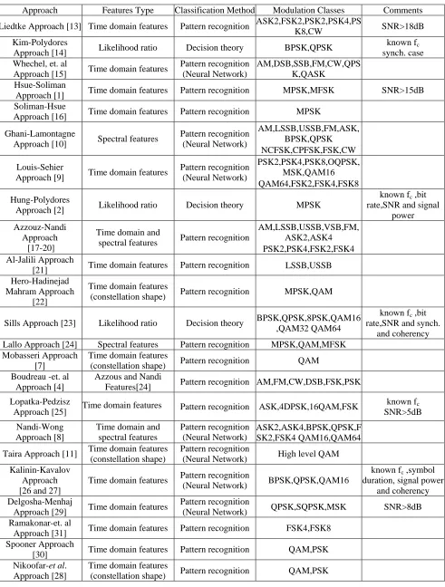
different methods for AMR introduced in the literature. Table 1 presents a brief review on the different approaches to the AMR problem.

Fig. 1. The input/output information relationship Fig. 2. The proposed input/output information relationship Most of these methods have been proposed for a limited number of modulations. For example,

extensive works are done to classify MPSK signals [1, 2, 5 and 16]. On the other hand each method uses

its own assumptions about the known parameters of the received signal such as carrier frequency, SNR,

baud rate and so on. So, combining different methods to recognize a broader class of modulation types is

not a simple task. Consider, for example, a method designed to classify MPSK signals and another method

for classification of MFSK signals. Besides any other different known and unknown parameter

assumptions, the former method assumes that input signals are solely PSK modulated, but with different

M. Therefore the response of the method to other signals, for example FSK signals, is not known. The

problem is more severe if the methods assume different previously known parameters like SNR or carrier

frequency.

The modulation set chosen in this paper includes AM, LSSB, USSB, FM, MASK, MPSK, MFSK all

for M=2, 4, 8 and MSK (minimum shift keying). According to Table 1 there are a number of different

methods to classify subsets of the above mentioned modulation schemes, but there is no method to

recognize all of these 14 modulation schemes. We use some of the features introduced previously in the

literature in our classification problem.

The above modulation schemes are selected from nine communication systems that we try to

recognize. We have chosen the systems with different modulation schemes in order to increase the

generality of our method. These systems are ACARS, ALE, ATIS, FMS-BOS, PACTOR-II, PSK31,

DGPS, GOLAY and ERMES. Successful recognition of these sample systems makes it easier to expand

our method to other communication systems. Table 2 gives a brief description of the chosen

communication systems.

The problem definition and introducing the selected features used in the proposed AMR method is

presented in Section 2. Section 3 is devoted to the proposed classifier which is a neural network. The

carrier and baud rate estimation and the proposed system recognition method is introduced in Section 4.

Results of simulation are presented in Section 5 and finally, conclusions are given in Section 6. Detection

AMR

Decoding

Protocol Recognition

Output Information

Input Information

Detection AMR

Decoding

Output Information

Table 1. Different approaches to the AMR problem Comments Modulation Classes Classification Method Features Type Approach SNR>18dB ASK2,FSK2,PSK2,PSK4,PS K8,CW Pattern recognition

Time domain features Liedtke Approach [13]

known fc

synch. case BPSK,QPSK Decision theory Likelihood ratio Kim-Polydores Approach [14] AM,DSB,SSB,FM,CW,QPS K,QASK Pattern recognition (Neural Network) Time domain features

Whechel, et. al Approach [15]

SNR>15dB MPSK,MFSK

Pattern recognition Time domain features

Hsue-Soliman Approach [1]

MPSK Pattern recognition

Time domain features Soliman-Hsue Approach [16] AM,LSSB,USSB,FM,ASK, BPSK,QPSK NCFSK,CPFSK,FSK,CW Pattern recognition (Neural Network) Spectral features Ghani-Lamontagne Approach [10] PSK2,PSK4,PSK8,OQPSK, MSK,QAM16 QAM64,FSK2,FSK4,FSK8 Pattern recognition (Neural Network) Time domain features

Louis-Sehier Approach [9]

known fc ,bit

rate,SNR and signal power MPSK Decision theory Likelihood ratio Hung-Polydores Approach [2] AM,LSSB,USSB,VSB,FM, ASK2,ASK4 PSK2,PSK4,FSK2,FSK4 Pattern recognition

Time domain and spectral features Azzouz-Nandi Approach [17-20] LSSB,USSB Pattern recognition

Time domain features Al-Jalili Approach

[21]

MPSK,QAM Pattern recognition

Time domain features (constellation shape) Hero-Hadinejad

Mahram Approach [22]

known fc ,bit

rate,SNR and synch. and coherency BPSK,QPSK,8PSK,QAM16

,QAM32 QAM64 Decision theory

Likelihood ratio Sills Approach [23]

MPSK,QAM,MFSK Pattern recognition

Spectral features Lallo Approach [24]

QAM Pattern recognition

Time domain features (constellation shape) Mobasseri Approach

[7]

AM,FM,CW,DSB,FSK,PSK Pattern recognition

Azzous and Nandi Features[24] Boudreau -et. al

Approach [4]

known fc

SNR>5dB ASK,4DPSK,16QAM,FSK

Pattern recognition Time domain features

Lopatka-Pedzisz Approach [25] ASK2,ASK4,BPSK,QPSK,F SK2,FSK4 QAM16,QAM64 Pattern recognition (Neural Network) Time domain and

spectral features Nandi-Wong

Approach [8]

High level QAM Pattern recognition

(Neural Network) Time domain features

(constellation shape) Taira Approach [11]

known fc ,symbol

duration, signal power and coherency BPSK,QPSK,QAM16

Pattern recognition (Neural Network) Time domain features

Kalinin-Kavalov Approach [26 and 27]

SNR>8dB QPSK,SQPSK,MSK

Pattern recognition (Neural Network) Time domain features

Delgosha-Menhaj Approach [29]

FSK4,FSK8 Pattern recognition

Time domain features Ramakonar-et. al

Approach [31]

QAM,PSK Pattern recognition

Time domain features Spooner Approach

[30]

QAM,PSK Pattern recognition

Time domain features (constellation shape) Nikoofar-et al.

Iranian Journal of Science & Technology, Volume 30, Number B6 December 2006

Table 2. The selected communication systems description

Application Frequency band Baud rate Comment Modulation System Aircraft Communication Addressing and Reporting System VHF 2400 BPS FSK-AM ACARS Automatic Link Establishment in HF

radio systems HF 125 BPS FSK-SSB ALE Automatic Transmitter Identification System in VHF-UHF radio systems VHF UHF 1200 BPS FSK F1=1300 HZ F2=2100 HZ FSK-FM ATIS radio signaling system for security

authorities and organizations VHF 1200 BPS FSK F1=1200 HZ F2=1800 HZ FSK-FM OR FSK FMS-BOS

a proprietary paging system VHF 300/600 BPS FSK GOLAY European Radio Message Standard VHF UHF 3125 BPS 4PAM-FM (4-FSK) ERMES data transmission system for radio

amateur use HF 100 BPS DBPSK DQPSK D8PSK PACTOR-II text conversations between two or more parties for radio amateur use HF 31.25 BPS DBPSK DQPSK PSK31 Differential Global Positioning System HF 100/200 BPS MSK DGPS

2. PROBLEM DEFINITION AND THE SELECTED FEATURES

Each type of modulation technique changes some parameters of the carrier signal according to the message to be sent. The main parameters of the carrier signal are frequency, phase and amplitude. So in order to recognize different modulation schemes, we should find some features that show the variation of these parameters.

FM and AM analog modulations are described according to the following formula [32]

y(t)=A[1+mx(t)]cos(2

π

f

_ct+

k

_d

∫

x

(

t

)

dt

) (1)

where m is the AM modulation depth, Kd is FM modulation index, x(t) is the modulating signal and fc is the carrier frequency.

The digital modulations are represented as [33]

MASK:

S

_m

(

t

)

=

Re[

A

_m

U

(

t

)

e

j2πfct

]

_m=1,2,..,M

MPSK:

(

)

Re[

(

)

( 1)]

]

2 2

[ + −

=

ft M m

m c

e

t

AU

t

S

π π

m=1,2, ..., M (2)

MFSK: m

(

)

Re[

(

)

j2 (f f )t

]

m c

e

t

AU

t

S

=

π + m=1,2,..,M

Minimum shift keying can be described as continuous phase modulation according to

MSK: ]

2 ) 4 1 ( 2 cos[ )

( _c I_n t n I_{n n}

T f A

t

Where

∑

−

−∞ =

=

n 1

k k

n

π

h

I

θ

,

I

_nare data amplitudes and h is called modulation index.

Now we need some features to show the variation in amplitude, phase and frequency of the received signal.

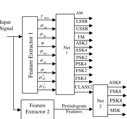
According to Table 1, many different features have been introduced previously toclassify subsets of the modulation schemes considered in this paper, but there is no method to recognize all of them simultaneously. So both time domain features introduced by Azzouz and Nandi [17] and spectral features proposed by Ghani and Lamontagne[10] are used for our classification problem. But there are some difficulties in combining the selected set of features in a way to make the proposed system efficient and reliable. Since we have used the neural networks as our classifier it is possible to use the hierarchical method for classification [9]. Therefore we consider AM, LSSB, USSB, FM, ASK2, ASK4, PSK2, PSK4, FSK2 and FSK4 as metagroup1 and the remaining ones (ASK8, PSK8, FSK8 and MSK) as metagroup2. We use two different neural networks with two different features for the two mentioned metagroups. The first neural network classifies the received signal in AM, LSSB, USSB, FM, ASK2, ASK4, PSK2, PSK4, FSK2, FSK4 and metagroup2. If the signal is classified as metagroup2 by the first neural network (Fig. 3), then the second neural network classifies it in ASK8, PSK8, FSK8 and MSK.

For metagroup1 we use the nine time domain features proposed by Azzouz and Nandi [17] which are described in Table 3 and are evaluated as follows:

1-

max

DFT

(

a

cn

(

i

))

/

Ns

2

max

=

γ

(4)

Ns : Number of samples per block

cn

a

: Normalized-centered instantaneous amplitude

2-

∑

∑

> > φ − φ = σ t

n i a n t

a a i a

NL NL

ap c i c i

) ( () 2 2 ) ) ( / 1 ( )) ( ( /

1 (5)

NL

φ

: Centered-nonlinear component of instantaneous phase, C: Number of samples in

φ

_NL for which

n

a

(i) >

a

_t, the threshold value of

)) ( ( ) ( ) ( i a mean i a i

a_n = and a(i) is the instantaneous amplitude.

3-

∑

∑

> > φ − φ = σ t

n i a n t

a a i a

NL NL

dp c i c i

) ( () 2 2 )) ( / 1 ( )) ( ( /

1 (6)

4- U L U L P P P P P + −

= (7)

where

∑

= = fcn i c

L X i

P 1 2 ) ( ,

∑

= + + = fcn i cn c

U X i f

P 1

2 ) 1

( ,

=

−

1

S S c cn

f

N

f

f

)

(

i

X

_c : Fourier transform of RF signal

5- 2

1 1 2 ) ) ( / 1 ( )) ( ( /

1

∑

∑

= = − = Ns i cn Ns i cn

aa Ns a i Ns a i

σ (8)

6- 2

) ( ) ( 2 ) ) ( / 1 ( )) ( ( /

1

∑

∑

> > − = σ t n t

n a i a

N a

i a

N

Iranian Journal of Science & Technology, Volume 30, Number B6 December 2006

)

(

i

f

N : Normalized-centered instantaneous frequency

7- 2 ) ( ) ( 2 ) ) ( / 1 ( )) ( ( /

1

∑

∑

> > − = σ t n t

n a i a

cn a

i a

cn

a c a i c a i (10)

8- 2 2 4 42 )}} ( { { )} ( { i a E i a E cn cn a ₌

µ (11)

where E{} means Expected value.

9- 2 2 4 42 )}} ( { { )} ( { i f E i f E N N f =

µ (12)

N

f

: Normalized-centered instantaneous frequency

Table 3. Time domain features [17] Description Feature

Maximum value of the spectral power density of the normalized-centered instantaneous amplitude of the signal

max

γ

Standard deviation of the absolute value of the centered non-linear component of the instantaneous phase, evaluated over the non-weak intervals of the signal ap

σ

Standard deviation of the centered non-linear component of the instantaneous phase, evaluated over the non-weak intervals of the signal

dp

σ

Is used for measuring the spectrum symmetry around the carrier frequency

P

Standard deviation of the absolute value of the normalized- centered instantaneous amplitude of the signal

aa

σ

Standard deviation of the absolute value of the normalized-centered instantaneous frequency, evaluated over the non-weak intervals of the signal

af

σ

Standard deviation of the normalized-centered instantaneous amplitude, evaluated over the non-weak intervals of the signal

a

σ

Kurtosis of the normalized-centered instantaneous amplitude of the signal a

42

µ

Kurtosis of the normalized-centered instantaneous frequency of the signal f

42

µ

For the second metagroup we use the spectrum of the signal as the feature as proposed in [10]. In this neural network, the Welsh periodogram of the signal is used as a feature for classification. To reduce the dimension of the input data, the main lobe of the periodogram containing most of the information is used and the remaining parts are discarded. The proper interval of periodogram is chosen after checking all the modulation set spectrums. It is trivial that signals with a higher bit rate will take more bandwidth than lower bit rates. Therefore, in order to choose the proper interval of the spectrum, the highest bit rate in our data base, which belongs to ERMES protocol (3125 bps), is considered. We have used 256 point FFT and it seems that a 6 point interval around a carrier frequency which has a 28.125 KHz bandwidth contains the proper portion of the main lobe. Hence we are sure that the selected interval will contain the main lobe of the spectrum of other systems with lower bit rates.

3. NEURAL NETWORK STRUCTURE

We have used the concept of hierarchical neural networks described in [9]. In this method classification can be done in successive steps. The outputs can be classified in groups called metagroups and the neural network classifies these metagroups first. Then classification can be done within each metagroup in the same manner. Our neural network classifies two metagroups mentioned in part 2. The input data is classified as one of the first metagroup members or just as metagroup 2. So we do not need an additional neural network for classification of the first metagroup subsets, however signals belonging to the second metagroup are classified to the final output result using another neural network structure. This method is shown in Fig. 3.

In Fig. 3, Net1 is a feed forward neural network with two hidden layers. The structure is chosen after extensive simulation tests. The number of nodes is 9 in the input layer, 75 in the first hidden layer, 75 in the second hidden layer and 11 in the output layer. The number of nodes is chosen to get the best performance results. The activation function used is log-sigmoid in the input and two hidden layers and a pure linear function in the output layer. The network is trained using a variable rate back propagation learning algorithm [36]. This training scheme converges faster and avoids falling in a shallow minimum, leading to better results.

With standard steepest descent, the learning rate is held constant throughout training. The performance of the algorithm is very sensitive to the proper setting of the learning rate. If the learning rate is set too high, the algorithm can oscillate and become unstable. If the learning rate is too small, the algorithm takes too long to converge. It is not practical to determine the optimal setting for the learning rate before training, and, in fact, the optimal learning rate changes during the training process as the algorithm moves across the performance surface.

The performance of the steepest descent algorithm can be improved if we allow the learning rate to change during the training process. An adaptive learning rate attempts to keep the learning step size as large as possible while keeping learning stable. The learning rate is made responsive to the complexity of the local error surface.

In adaptive learning rate, the training procedure is as follows. First, the initial network output and error are calculated. At each epoch new weights and biases are calculated using the current learning rate. New outputs and errors are then calculated. If the new error exceeds the old error by more than a predefined ratio, (1.04 in our simulations), the new weights and biases are discarded. In addition, the learning rate is decreased (by multiplying by 0.7 in our simulations). Otherwise, the new weights, etc., are kept. If the new error is less than the old error, the learning rate is increased (by multiplying by 1.05 in our simulations). This procedure increases the learning rate, but only to the extent that the network can learn without large error increases.

The second neural network named Net2 in Fig. 3 is a one hidden layer feed forward neural network that is trained using the same method as Net1. It has only one input node. There are 80 nodes in its hidden layer and log-sigmoid function is used in its input and the hidden layer and a pure linear function in the output layer.

Iranian Journal of Science & Technology, Volume 30, Number B6 December 2006

Fig. 3. The neural network structure used in our method 4. SYSTEM RECOGNITION

Figure 4a depicts the general block diagram of the proposed signal intercept system. As this figure shows, the whole expected radio frequency (RF) spectrum is searched for signal presence using a scanning energy detector receiver. As soon as the presence of a signal is detected (S1(t)), its frequency band is down converted to intermediate frequency (IF). In this step we have only a rough estimate of the carrier frequency(fRF). The IF signal (S2(t)) is processed by an AMR block using the presented algorithms of Sections 2 and 3. The precise carrier frequency is also estimated (fc). For carrier frequency estimation we have used the zero crossing method of [1] with some modifications. Using the recognized modulation type (Mod. Typ.) and the estimated carrier frequency (fc) the demodulated signal can be derived (x[n]).

The system recognition block in Fig. 4a, uses fc , fRF , Mod. Typ. and x[n] and recognizes the communication system type.

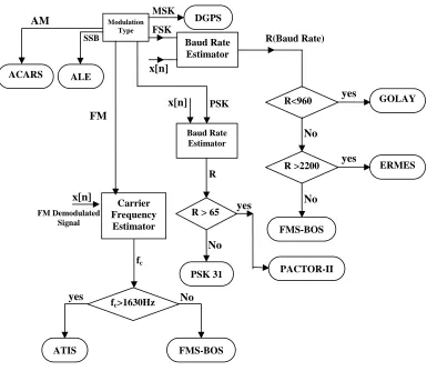
The main features of the 9 systems used in the system recognition process (modulation scheme, bit rate and carrier frequency) are presented in Table 2. Further details can be found in [35]. Fig. 4.b shows the proposed system recognition decision tree. In the proposed scheme we need two main blocks, baud rate estimator and carrier frequency estimator.

For carrier frequency estimation we have used the zero crossing method of [1] with some modifications and the baud rate is estimated using the method proposed in [34].

Using the recognized modulation type, estimated carrier frequency and baud rate, the system can be recognized using the decision tree given in Fig. 4.b. It should be noted that according to Table 2, some of the systems use two-step modulations. For example ACARS (Aircraft Communication Addressing and Reporting System) uses FSK modulation for base band modulation of data and then AM modulates the resultant signal in VHF band. FMS-BOS also uses a two-step modulation FSK-FM. In these cases the final modulation type is recognized and the system can be recognized by processing the demodulated signal.

It can be seen that our proposed AMR algorithm can recognize more modulation classes than are used in the 9 communication systems of Table 2. So, although we considered nine classes of communication systems in this research, expanding the number of classes is straightforward using the principles given here. According to Fig. 4, it can be seen that the main source of error in system classification is the AMR error. Due to a large difference in baud rate or carrier frequency, the classification based on these two parameters has a negligible error relative to the AMR error( The simulations show that for SNR>15dB the classification error between ATIS and FMS-BOS due to the carrier frequency estimation error is less than 0.5 percent and the baud rate classification error is almost zero). So in the next section we solely present the performance of the AMR algorithm.

Feature

Ext

ractor 1 Net 1 max

γ

ap

σ

dp

σ

P

aa

σ

af

σ

a

σ

a 42

µ

f 42

µ

LSSB USSB FM ASK2 ASK4 PSK2 PSK4 FSK2 FSK4 CLASS2

Net 2

ASK8 FSK8

MSK PSK8 Periodogram

Features

AM

Feature Extractor 2 Input

Fig. 4. a) Block diagram of the signal intercept system

Fig. 4. b) System recognition decision tree

5. SIMULATION RESULTS

For simulation we choose an IF frequency equal to 150 KHz for our simulations. Two parameters which affect the selection of IF frequency are baud rate and the modulation type. The highest baud rate has the widest spectrum and the modulation type also affects the spectrum width. In our case 150 KHz value for IF frequency is chosen according to these parameters. The IF signals are sampled with a 1200 KHz sampling frequency which is high enough to avoid aliasing. In order to make our decision more reliable, at least a few bits of information should be received.

AMR Block

Carrier Frequency Estimation

@IF

Demodulator Scanning

Receiver

) (

1 t

s : Input Signal

System Recognition

) (

2 t

s : IF Signal _{Mod. Typ.}

Estimated RF Frequency

RF

f

c

f

X[n]: demodulated signal

c

f

System Type Mod. Typ.

Modulation Type

ALE ACARS

Carrier Frequency

Estimator

fc>1630Hz

ATIS FMS-BOS

Baud Rate Estimator

R > 65

PSK 31 PACTOR-II

Baud Rate Estimator DGPS

R<960

R >2200

GOLAY

ERMES

FMS-BOS

yes No

No No

yes

yes

yes

No

R

fc

x[n]

R(Baud Rate)

AM

x[n] x[n]

MSK

FSK

SSB

PSK

FM

Iranian Journal of Science & Technology, Volume 30, Number B6 December 2006

Two separate sets of signals have been used for training and testing the neural network. The results are presented in Tables 4 and 5. It should be mentioned that the results have been evaluated considering 20 frames of signal in each SNR. In Tables 4 and 5 the performance of the neural network for Class1 and 2 signals is presented separately. The whole performance has been shown in Table 6.

Table 4. The percent of correct decision probability of the first class

SNR(dB) 0 5 15 25 35 45 55

AM 87.51 90 90 100 100 100 100

LSSB 15 55.5 90 100 100 100 100

USSB 17 85.7 95 100 100 100 100

FM 90 85 90 100 100 100 100

ASK2 90 100 100 100 100 100 100

ASK4 80 100 100 100 100 100 100

PSK2 10 35 80 100 100 100 100

PSK4 15 65 95 100 100 100 100

FSK2 85 75 100 100 100 100 100

FSK4 75 100 100 100 100 100 100

Table 5. The correct decision probability of the second class SNR 0 dB 5 dB 15 dB 25 dB 35 dB 45 dB 55 dB ASK8 15 60 80 100 100 100 100

PSK8 45 70 90 95 100 100 100

FSK8 30 75 87.5 97 100 100 100

MSK 20 60 95 100 100 100 100 Table 6. Simulation results: Input modulations vs. deduced modulations at 15dB SNR

Input

Modulation Recognized Modulation scheme

AM LSSB USSB FM MASK MPSK MFSK MSK

AM 90% - - - 10% - - -

LSSB - 90% - - - 5.5% 3.5% 1%

USSB - - 95% - - 4% 1% -

FM - - - 90% - - 10% -

ASK2 - - - - 100% - - -

ASK4 - - - - 100% - - -

ASK8 20% - - - 80% - - -

PSK2 - - - - - 80%-20%(error) - -

PSK4 - - - - - 95%-5%(error) - -

PSK8 - - - - - 90%-10%(error) - -

FSK2 - - - - - - 100% -

FSK4 - - - - - - 100% -

FSK8 - - - 13.5% - - 87.5% -

MSK - - - 0.5% - - 4.5% 95%

Table 7. Comparison of our method with Azouz[17] and Ghani[10] at 15 dB SNR

AM LSSB USSB FM ASK2 ASK4 PSK2 PSK4 FSK2 FSK4 Azzouz [17] 88.5 99.8 98.5 90.1 96.8 86.5 99.5 96.8 99 99.5 Ghani [10] 97.1 99.2 99 89.9 96.1 --- 96.8 99.1 100 ---

Our Method 90 90 95 90 100 100 85 95 100 100

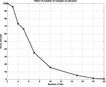
We have also investigated the result of the reduction of the frame length. As one might expect, reducing the frame length decreases the number of bits of information in the frame and can reduce our decision reliability drastically. The results shown in Fig. 5 indicate that, the number of bits less than 5 makes the correct decision impossible. Although this figure has been obtained for PSK31 protocol with 31.25 baud, it can be used as a figure of merit for all other protocols too. In the simulations corresponding to Fig. 5, for testing the effect of the number of received bits on the decision, we assumed a noise-less channel, so the result does not contain the effect of SNR levels.

Fig. 5. Effect of number of bits on decision error

Figure 6 shows the effect of the number of frames on decision errors. Because the decision is made on a frame basis, it is expected that integrating the decision results on more frames will increase the accuracy. In this situation, although each frame is classified independently by the neural network as a modulation type, a group of frames are considered together for integration before final decision making. As the number of frames in the integration process increases, the error reduces.

Iranian Journal of Science & Technology, Volume 30, Number B6 December 2006

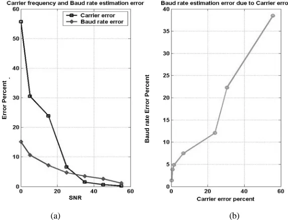
The next step is to estimate carrier frequency and baud rate. Using the methods mentioned in Section 4, the carrier frequency and baud rate can be estimated effectively in SNRs above 15 dB. Fig. 7 shows both carrier frequency and baud rate RMS(root mean square) estimation error in percentage. In Fig. 7a the performance of the baud rate estimator is considered against noise where carrier frequency is assumed to be known exactly. But in Fig. 7b the effect of carrier frequency estimation error on the performance of the baud rate estimator is evaluated. In this figure the noise is not considered. The results are obtained for a carrier frequency equal to 150 KHz, and obviously depend on the carrier frequency. But it can be seen that the performance of the baud rate estimator decreases as the carrier frequency estimation error increases.

(a) (b) Fig. 7. Carrier frequency and baud rate estimation error

In our application the baud rate estimation error is not as important as the carrier frequency estimation error. A rough estimation of the baud rate can be used in the system database table to match the nearest value. However the effect of the estimation error of the carrier frequency is more severe. This is why the simple but fast baud rate estimator of [34] can be effectively used in our method.

Using the recognized modulation scheme and estimated baud rate and carrier frequency and comparing this information with the known expected values for the nine systems mentioned earlier, the protocol can be recognized.

6. CONCLUSION

We have developed a method for recognition of communication systems based on modulation recognition and baud rate and carrier frequency estimation. For automatic modulation recognition we have developed a new method based on two different sets of features which have been proposed in the literature for different applications, to recognize a wide set of 14 modulation schemes. These modulation schemes have not been considered together in a classification problem previously. The proposed AMR method does not need a prior knowledge of SNR, carrier phase and symbol rate. The classification procedure is performed by the hierarchical neural network. The back propagation training method with a variable learning rate is used. Simulation results show that the overall performance of the AMR method used in this paper is above 75%, even in SNR as low as 5 dB. For SNR above 35 dB, the performance reaches 100%. Although we considered nine classes of communication systems in this research, expanding the number of classes is straightforward using the principles given here.

Error Per

cent

Baud rate Error

Per

c

Acknowledgement- The authors would like to thank A. Zamani for his contribution to this work.

REFERENCES

1. Hsue, S. Z. & Soliman, S. S. (1989). Automatic modulation recognition of digitally modulated signals. MILCOM Conf., Boston, MA, ‘89, 3, 645–649.

2. Hung, C. Y. & Polydoros, A. (1995). Likelihood methods for MPSK modulation classification. IEEE Trans. On Communication, 1, COM 43(2/3/4), 1493–1503.

3. Polydoros, A. & Kim, K. (1990). On detection and classification of quadrature digital modulations in broad-band noise. IEEE Trans. On Communication, 38(8), 1199–1211.

4. Boudreau, D., Dubuc, C. & Patenaude, F. (2000). A fast automatic modulation recognition algorithm and its implementation in a spectrum monitoring application, MILCOM, Conf.,2, Los Angeles, CA, OCT., 732-736.

5. Hong, L. & Ho, K. C. (2000). BPSK and QPSK modulation classification with unknown signal levels. MILCOM, Conf., Los Angeles, CA, Oct., 2, 976-980.

6. Lichun, L. (2002). Comments on signal classification using statistical moments. IEEE Trans. On Communication, 50(2), 1199–1211.

7. Mobasseri, B. (2000). Digital modulation classification using constellation shape. Signal Processing, Jan., 80(2), 251-277.

8. Wong, M. L. D. & Nandi, A. K. (2001). Automatic modulation recognition using spectral and statistical features with multi layer perceptrons. Sixth International Symposium on Signal processing and its Application, Kuala Lumpur, 2, Aug., 390-393.

9. Louis, C. & Sehier, P. (1994). Automatic modulation recognition with hierarchical neural networks. MILCOM, Conf., 3, Malaysia, Fort Monmouth, NJ, Oct., 713-717.

10. Ghani, N. & Lamontagne, R. (1993). Neural networks applied to the classification of spectral features for automatic modulation recognition. MILCOM,Conf., 1, Boston, MA, Oct., 111-115.

11. Taira, S. (2001). Automatic classification of QAM signals by neural networks. in Proc. ICASSP 2, Salt Lake City, Utah, May, 1309–1312.

12. Delgosha, F. (1998). Digital modulation recognition. Master’s Thesis, Sharif University of Technology.

13. Liedtke, F. F. (1984). Computer simulation of an automatic classification procedure for digitally modulated communication signals with unknown parameters. Signal Processing, August, 6(4), 311-323.

14. Kim, K. & Polydoros, A. (1988). Digital modulation classification: the BPSK versus QPSK case. MILCOM, Conf. 2, San Diego, California, Oct., 431-436.

15. Whelchel, J. E., McNeill, D. L., Hughes, R. D. & Loos, M. M. (1989). Signal understanding: An artificial intelligence approach to modulation classification. Tools for Artificial Intelligence: Architectures, Languages and Tools, IEEE international Conf., Fairfax, VA, Oct. 231-236.

16. Soliman, S. S. & Hsue, S. (1992). Signal classification using statistical moments. IEEE Trans. On Communication,

COM 40(5), May, 908-916.

17. Azzouz, E. E. & Nandi, A. K. (1996). Automatic modulation recognition of communication signals. Kluwer Academic Publishers, Boston.

18. Nandi, A. K. & Azzouz, E. E. (1998). Algorithms for automatic modulation recognition of communication signals.

IEEE Trans. On Communication, 46(4), 431-436.

19. Nandi, A. K. & Azzouz, E. E. (1995). Automatic analogue modulation recognition. Signal Processing, 46, 211-222. 20. Azzouz, E. E. & Nandi, A. K. (1995). Automatic identification of digital modulation types. Signal Processing, 47,

55-69.

Iranian Journal of Science & Technology, Volume 30, Number B6 December 2006

22. Hero, A. O. & Hadinejad-Mahram, H. (1998). Digital modulation classification using power moment matrices.

Acoustics, Speech and Signal Processing, IEEE International Conf. on, ICASSP 98, Vol. 6, Seattle, Washington, USA, 12-15 May, 3285-3288.

23. Sills, J. A. (1999). Maximum-likelihood modulation classification for PSK/QAM. MILCOM Conf., 1, Atlantic City, NJ, 31Oct.-3Nov., 217-220.

24. Lallo, P. (1999). Signal classification by discrete Fourier transform. MILCOM Conf. Proceedings, 1, Atlantic City, NJ, 31Oct.-3Nov., 197-201.

25. Lopatka, J. & Pedzisz, M. (2000). Automatic modulation classification using statistical moments and a fuzzy classifier. Signal Processing Proceedings,WCCC- ICSP 2000, 5th International Conf., Beijing, China, Aug. 3, 1500-1506.

26. Kalinin, V. & Kavalov, D. (2000). Application of SAW artificial neural network processor to digital modulations.

Ultrasonics Symposium, 1, San Juan, Puerto Rico, Oct., 51-54.

27. Kavalov, D. & Kalinin, V. (2001). Improved noise characteristics of SAW artificial neural network RF signal processor for modulation recognition. Ultrasonics Symposium, 1, Oct., Atlanta, USA, 19-21.

28. Nikoofar, H. R., Sherafat, A. R. & Shahmohammadi, M. (2002). Modulation recognition for PSK/QAM signals using constellation features and soft clustering. ICEE, Tabriz, IRAN, 338-344 (in Persian).

29. Delgosha, F. & Menhaj, M. B. (2001). Amplitude-based neuro-classifier for classification of digital quadrature and staggered modulations. Neural Networks, Proceedings, IJCNN ’01, International Joint Conf., 1, Washington DC, USA, July, 721-725.

30. Spooner, C. M. (2001). On the utility of sixth-order cyclic cumulants for RF signal classification. Conf. Record of Thirty-Fifth Asilomar Conference, on Signals, Systems and Computers, 1, Pacific Grove, CA, Nov., 890-897. 31. Ramakonar, V., Habibi, D. & Bouzerdoum, A. (2001). Classification of bandlimited FSK4 and FSK8 signals.

Signal Processing and its Applications, Sixth International symposium, 2, Kuala Lumpur, Malaysia, Aug., 398-401. 32. Carlson, A. B., Crilly, P. B. & Rutledge, J. C. (2001). Communication systems. McGraw Hill, Fourth edition. 33. Proakis, J. G. (1989). Digital communication. McGraw Hill international edition, Second edition.

34. Wegener, A. W. (1992). Practical techniques for baud rate estimation. ICASSP-92, 4, San Francisco, CA, Mar., 681-684.

35. Attar, A. R. (2004). Modulation and protocol recognition in military communication system. Master’s Thesis, Shiraz University.