Robust Control of Encoderless Synchronous Reluctance
Motor Drives Based on Adaptive Backstepping and
Input-Output Feedback Linearization Techniques
Jafar Soltanii and Hossein Abootorabi Zarchiii*
i Jafar Soltani is with the Faculty of Engineering, Islamic Azad University, Khomeini-shahr Branch, Esfahan, Iran (e-mail: [email protected]). ii* Corresponding Author, Hossein Abootorabi Zarchi is with the Faculty of Engineering, Ferdowsi University of Mashhad, Mashhad, Iran (e-mail: [email protected]).
ABSTRACT
In this paper, the design and implementation of adaptive speed controller for a sensorless synchronous reluctance motor (SynRM) drive system is proposed. A combination of well-known adaptive input-output feedback linearization (AIOFL) and adaptive backstepping (ABS) techniques are used for speed tracking control of SynRM. The AIOFL controller is capable of estimating motor two-axis inductances (Ld, Lq), simultaneously. The overall stability of the proposed control and Persistency of Excitation (PE) condition are proved based on Lyapunov theory. In the proposed control drive system, the maximum torque control (MTC) scheme and constant current in inductive axis control (CCIAC) are applied to generate the motor d and q axis reference currents which are needed for the AIOFL controller. In addition, an ABS speed controller is designed to compensate for the machine parameter uncertainties and load torque disturbances. Another contribution of this paper is to estimate the rotor speed and position in very low speed by using 1) a simple technique for eliminating the voltage sensors, 2) a simple method for online estimation of the stator resistance, and 3) modeling the voltage drop of the inverter power switches. Finally, the validity and capability of the proposed method are verified through simulation and experimental studies.
KEYWORDS
Synchronous Reluctance Motor, Adaptive Backstepping and Input-Output Feedback Linearization, Encoderless
1. INTRODUCTION
The SynRM is one of the oldest and simplest types of electric motors. In recent years, it has been shown that SynRM can be competitive with other ac motors [1-6]. A SynRM is advantaged on induction motor by the absence of rotor copper losses, on brushless motors by inexpensive rotor structure and on switched reluctance motor by a much lower torque ripple and low noise.
In the last two decades, the SynRM parameter identification has been challenging so that some researchers have tried to solve this problem [7-10]. One may notice that uncertainties and variations of the parameters seriously affect the motor performance specially its closed-loop control stability. In Off-line parameter identification methods described in [7, 8], the SynRM electrical parameters are obtained for some operating points by practical tests and inserted in look-up tables or mathematically approximated by some curves. An alternative solution is on-line estimation of the
machine parameters [9, 10]. In [9, 10], SynRM electrical parameters (Ld, Lq, Rs)are estimated using the Recursive Least-Squares estimator (RLSE). It is not necessary to say that RLSEat each ∆tstep of time needs to reset a so-called positive definite co-variance matrix, which results in a high computation storage and time [11]. Authors of [9] have described in their paper that although is possible to estimate all the electrical machine parameters by the RLS method, the estimator performance is considerably improved if only Ld is estimated with the assumption of constant Rs and Lq.
EEMF observer as well as the motor controller. In this approach, the RLS estimator needs to know the motor estimated speed and measured currents and voltages. One may note that in the method of [10], the rotor speed is estimated by derivation of θˆr which is the output of the
EEMF observer. The overall stability of such very complicated system is dubious and really cannot be analytically proved. As mentioned in [10], by this method the low speed estimation is impossible; however, the authors of [10] have claimed that the motor speed estimation is possible above 50 rpm while no any practical results have been proposed for such a claim. The practical results given in [10] show possibility the motor speed estimation only from 500 rpm to 1000 rpm. In [12], a predictive direct torque control has been presented for encoderless SynRM which is able to operate at low speeds. At the low speed operation, the rotor angular position is estimated by injecting test voltage signals (TVSs) to detect the spatial orientations of existing position-dependent rotor anisotropies. However, the TVSs deteriorate the performance of the predictive algorithm, and they create some audible noise. The method of [12] is complicated and for each motor chosen it is required to obtain the motor inductances by off-line methods.
The main contribution of this paper is to use the well-known adaptive input-output feedback linearization (AIOFL) and adaptive backstepping (ABS) techniques for SynRM robust speed control without using any mechanical position sensor and voltage sensor with simultaneous estimation of d and q axis inductances (Ld, Lq). Backstepping is a recently developed design tool for constructing globally stabilizing control laws for a certain class of nonlinear dynamic systems with a lower triangular structure. The persistency of excitation (PE) is proved in the paper. In the proposed control technique, we need to know the motor d and q axis reference currents ( * *
, qs ds i
i ). These reference currents are generated based on
Maximum Torque Control (MTC) and id constant strategies. By our control approach, the rotor speed estimation is possible. One may note that in the rotor low speed estimation, we have some problems such as voltage and current sensors dc offsets as well as the slowly variation of stator resistance with temperature. We solve these problems by 1) using a simple method for eliminating the voltage sensors, 2) a simple method for an online estimation of the stator resistance, and 3) using a PI estimator and modeling the voltage drop of the inverter power switches. It is worth to mention that the current sensors dc offsets observed on the measured currents are negligible.
2. THE SYNRMMODEL
The SynRM d-q axis equations in the rotor reference frame taken into account cage winding is given by [13]
(1) q
e ds ds s ds
dt d i R
v = + λ −ω λ
(2) d
e qs qs s qs
dt d i R
v = + λ +ω λ
(3)
dt d i dr
dr
λ
+ =Rdr
0
(4)
dt d iqr+ λqr
=Rqr 0
with
(5)
ls mq q ls md d
dr ds md dr ds ls dr ds md ds
qr qs mq qr qs ls qr qs mq qs
L L L L L L
i i L i
L i i L
i i L i
L i i L
+ = +
=
+ + =
+ + =
+ + =
+ + =
,
) ( ,
) (
) ( ,
) (
λ λ
λ λ
In the above, λdsandλqsare stator linkage fluxes,
ds
v andvqsare stator voltages,
i
dsandi
qsare stator currents;i
drandi
qrare rotor currents, LmdandLmqdenote mutual inductances, Llsis stator leakage;LldrandLlqr are rotor leakages, LdandLqare stator inductances,dr
R andRqrare rotor resistances, all in d and q axis rotor reference frame. Rsis the stator resistance and
ω
eis the rotor electrical angular velocity. From Eqs. (1-5) the equivalent circuits of SynRM can be represented by Fig. 1. In addition, the motor generated torque is(6)
( 2 2 3 ) ( 2 2 3
) (
2 2 3
qr mq qr dr md qs
ds q d
ds q qs d
i i L i i L P i i L L P
i i P Te
− +
− =
−
= λ λ
where
P
is number of poles. Finally, the motormechanical equations are
(7)
m m l e m m m m
dt d T T B dt d
J ω + ω = − , θ =ω
where Jm is the rotor moment of inertia, Bm is the friction coefficient, θm is the rotor displacement angle in mechanical degrees, ωm is the rotor mechanical angular
velocity and Tl denotes the motor load torque.
3. ADAPTIVE INPUT-OUTPUT FEEDBACK
LINEARIZATION
Figure 1: Equivalent d-q axis circuits of the SynRM with cage.
IOFL for SynRM drive system in order to obtain the reference space voltage vector for the SV-PWM inverter which feeds the motor [14-16].
For this purpose, ignoring the cage rotor of SynRM in Fig.1 and choosing
λ
ds ,λ
qs andω
e as state variablesand assuming vds =u1 and vqs =u2 as the system
control efforts, the nonlinear model is described by
(8)
U
X
g
X
f
X
=
(
)
+
(
)
where
(9)
[
]
T[
]
Te qs ds T u u U x x x
X= 1 2 3 =[λ λ ω] , = 1 2
(10) , 2 / ) 1 1 4 3 ( ) ( 3 2 1 ⎥ ⎥ ⎥ ⎥ ⎥ ⎥ ⎥ ⎦ ⎤ ⎢ ⎢ ⎢ ⎢ ⎢ ⎢ ⎢ ⎣ ⎡ − − ⎟ ⎟ ⎠ ⎞ ⎜ ⎜ ⎝ ⎛ − − − + − = ⎥ ⎥ ⎥ ⎦ ⎤ ⎢ ⎢ ⎢ ⎣ ⎡ = m e m m l qs ds d q m e ds d qs s e qs q ds s J B P J T L L J P i L i R i L i R f f f X f ω λ λ ω ω and (11) [ ] , 0 0 1 0 0 1 )
( 1 2
⎥ ⎥ ⎥ ⎦ ⎤ ⎢ ⎢ ⎢ ⎣ ⎡ = = g g X g
Introducing the following output variables
(12)
1 ds, 2 qs,
y = λ y = λ
from (1), the system output dynamics can be obtained as (13) U X E f f u u f f y y ) ( 1 0 0 1 2 1 2 1 2 1 2 1 + ⎥ ⎦ ⎤ ⎢ ⎣ ⎡ = ⎥ ⎦ ⎤ ⎢ ⎣ ⎡ ⎥ ⎦ ⎤ ⎢ ⎣ ⎡ + ⎥ ⎦ ⎤ ⎢ ⎣ ⎡ = ⎥ ⎦ ⎤ ⎢ ⎣ ⎡
From (8-13), an internal dynamics is recognized that its stability can be easily proved [11]. Based on the input– output feedback linearization, the control effort is
(14) ⎥ ⎦ ⎤ ⎢ ⎣ ⎡ − − = − 2 2 1 1 1 f v f v E U
Assuming the new state variables as
(15) 2 2 1 1 v y v y = =
The system control efforts are defined by
(16) ds qs q e ds s d ds v i L i R e dt d
v =
λ
−α
1 =− +ω
+* 1 (17) qs ds d e qs s q qs v i L i R e dt d
v = λ −α2 =− −ω +
*
2
where
α
1 andα
2 are positive constant and* *
,
q qs qsds ds
d
e
e
=
λ
−
λ
=
λ
−
λ
. The superscript “*”denotes the reference value.
Using (16) and (17), the motor estimated model is
(18) ds qs e ds s d
ds e R i ai v
dt d
v = − 1 =− + 2 +
*
1
α
ω
ˆλ
(19) qs d e qs s q qs v i a i R e dt dv = − 2 =− − 1 +
*
2
α
ω
ˆλ
where aˆ1=Lˆd andaˆ2 =Lˆq are estimated values of
1
a
anda
2, respectively.From (15), (18) and (19), the motor error dynamics becomes (20) q q d d e dt de e dt de 2
1 , α
α =−
− =
This equation shows that for positive
α
1 andα
2,e
dand
e
q exponentially converge to zero.4. ADAPTATION LAW
Assume that (21)
;
ˆ
~
;
ˆ
~
2 2 2 1 11
a
a
a
a
a
a
=
−
=
−
where
a
~
1 anda
~
2 are the error values between the actual and estimated parameters.From Eqns. (13), (18) and (19), one can have
(22) d qs e d d ds qs e ds qs q e ds s ds e a i e e a i v v v i L i R 1 2 1 * 2 1 1 ~ ~ ) (
α
ω
α
λ
ω
ω
λ
− = ⇒ − + = + − + + − = and (23) q ds e q q qs ds e qs ds d e qs s qs e a i e e a i v v v i L i R 2 1 2 * 1 2 2 ~ ~ ) (α
ω
α
λ
ω
ω
λ
− − = ⇒ − + − = + − + − − =Eqs. (22) and (23) in a matrix compact form as
a) d-axis Equivalent Circuit
(24)
θ
~
T
W
Ax
x
=
+
where
x
=
[
e
de
q]
T,[
a~1 a~2]
T~=
θ
,⎥
⎦
⎤
⎢
⎣
⎡
−
−
=
2 1
0
0
α
α
A
with
⎟⎟
⎠
⎞
⎜⎜
⎝
⎛
−
=
0
i
i
0
ds e
qs e
ω
ω
T
W
.The following Lyapunov function is used
(25)
θ
θ
~
~
2
1
2
1
+
Γ
−1=
x
Tx
TV
where
Γ
=
diag
[
γ
1,
γ
2]
.1
γ
andγ
2 are positive adaptation gains. The Derivate ofV
with respect to time t is(26)
θ
θ
θ
=
T+
~
T+
~
TΓ
−1~
Wx
x
A
x
V
Assume the following adaptation law
(27)
Wx
Γ
−
=
θ
~
Then (26) is changed to
(28)
x
A
x
V
=
TSince A is a negative definite matrix, therefore from (28),
(29)
0
≤
V
d
L
andL
qare assumed to be unknown constantparameters, hence
(30) 1
1
ˆ
~
a
a
=
−
,a
~
2=
−
a
ˆ
2As a result from (27), the adaptation laws are obtained as
(31) q
ds
e
i
e
a
ˆ
1=
−
γ
1ω
and
(32) d
qs
e
i
e
a
ˆ
2=
γ
2ω
One may note that V is a radially unbounded function, therefore (25) and (29) guarantee that
e
d ande
qarebounded. As a result from (24),
W
Tandx
are also bounded, too. From Barbalat’s Lemma [11], we have(33)
∞ → =
=0; lim 0 :for t
limed eq
Moreover, if there exist two positive real constants T and C such that the Persistency of Excitation (PE) condition
(34)
( )
( )
I2, for all t 0T t
t ≥ ≥
∫
+ W τ WT τ dτ Cis satisfied, then from [11] it follows that the estimation
error vector
θ
~
exponentially converges to zero. It meansthat
L
ˆ
d andL
ˆ
q finally reach to the actual values,respectively. This results in
( )
( )
t T
t
0 0
0.
0 0 e
t T T
t
W τ W τ dτ dτ for ω
+ + ⎛ ⎞
= ⎜ ⎟ =
⎝ ⎠
∫
∫
Hence, the matrix in (34) is positive semi-definite and the PE condition fails. When
ω
e≠
0
, we obtain( ) ( )
∫
∫
( )
∫
+ + ⎟⎟ = +⎠ ⎞ ⎜
⎜ ⎝ ⎛
= t T
t T
t t
qs ds T
d M d
i i d
W
W τ τ τ
ω ω τ
τ
τ 2 2
e 2 2 e T
t
t 0
0
Since M is positive definite therefore, the matrix in (34) is also positive definite. As a result, the PE condition is satisfied and consequently the estimation error vector θ~ exponentially converges to zero.
5. THE ADAPTIVE BACKSTEPPING SPEED CONTROLLER
From (7), it is not difficult to derive
(35)
[
]
1 2 31
r e l m r e l r
m
d
T T B A T A T A dtω =J − − ω = + + ω
with
1 2
1
m
A A
J
= = − ,
3
m
m B A
J
= −
where A1,A2 and A3 are constant parameters which are related to the motor parameters. In the real-world, unfortunately the parameters are varied by the saturated effect or temperature. As a result, it should be taken into account by the controller designer. In this paper, we propose an adaptive backstepping controller to compensate for the machine parameter uncertainties and load torque disturbances. Therefore,
(36)
1 3 2 1 2 3
1 3
( )
r e r l e l r
e r
d
A T A A T A T A T A
dt
A T A d
ω ω ω
ω
= + + + ∆ + ∆ + ∆
= + +
and
(37)
2 1 2 3
( l e l r)
d = A T + ∆A T + ∆A T + ∆Aω
where ∆A1,∆A2 and ∆A3 are the variations of the parameters and dis the uncertainty including the effects of the parameter variations and the external load.
Define the speed error e2 as
(38) r
r
e =ω*−ω 2
Taking the derivative of both sides of (38), it is easy to obtain
(39) r
r
e =ω*−ω 2
(40)
2 2 2 2
2 2
1 1 1 1 1 1 ˆ
( )
2 2 2 2
V e d e d d
γ γ
= + = + −
Taking the derivative of (18), it is easy to obtain
(41)
2 2 2 2 2 2
1
1
ˆ
1
ˆ
(
)
V e e
d d e e
d d d
e e
dd
γ
γ
γ
=
+
=
+
− =
−
By substituting (39) into (41) and doing some arrangements, we can obtain
(42) *
2 1 3
*
2 1 3
1 ˆ
(
)
1
ˆ
ˆ
(
)
rm e rm
rm e rm
V e
AT
A
d
d d
e
AT
A
d d
d d
ω
ω
γ
ω
ω
γ
=
−
−
− −
=
−
−
− − −
Assuming that the torque can satisfy the following equation
(43)
(
*)
3 2
1
1
ˆ
e rm rm
T
A
d
Me
A
ω
ω
=
−
− +
and substituting (43) into (42), we can obtain
(44) 2
2 2
1
ˆ
V
M e
d e
dd
γ
= −
−
−
From (44), it is possible to cancel out the last two terms by selecting the following adaptive law
(45) 2
ˆ
d
= −
γ
e
In (23), the convergence rate of
d
ˆ
is related to the parameterγ
. By submitting (45) into (44), we can obtain(46) 2
2
0
V
= −
Me
≤
From (46), we can conclude that the system is stable; however, we require to use Barbalet lemma to show that the system is asymptotical stable. By integrating (46), we can write
(47)
0
V d
τ
( ( )
V
V
(0))
∞
=
∞ −
< ∞
∫
From (47), the integration of parameter
e
22of (46) isnot infinite. Then, e2(t)∈L∞∩L2and e2(t)is bounded. According to the Barbalet lemma, we can conclude
(48) 2
lim
( )
0
t→∞
e t
=
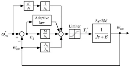
The block diagram of the proposed adaptive backstepping control system is shown in Fig. 2, which is obtained from (43) and (45).
Figure 2: Adaptive Backstepping Controller.
6. STATOR RESISTANCE ESTIMATION
The variation of the stator resistance is a thermal process and therefore is not only determined by the machine losses but also the time [17].
Among the machine variables, the stator flux vector is highly affected by the resistance changes particularly at low speed. In addition, the IOFL controller can be made more reliable if the stator resistance is estimated online during operation of the machine. In this paper, a PI estimator is employed based on comparing the actual current and the reference current to predict the stator resistance [17, 18]. As shown in Fig. 3, the error in the stator current is used as an input to the PI estimator. The technique is based on the principle that the error between the actual stator current and the reference current is proportional to the stator resistance change [17]. The PI resistance estimator is described by
(49) s
I P
s I
s K K
R ⎟∆
⎠ ⎞ ⎜
⎝
⎛ +
= ∆
where the letter "s" is the Laplace operator andKP and I
K are the proportional and integral gains of the PI estimator. The error between the actual stator current and its reference is passed through a low pass filter with a very low cutoff frequency in order to attenuate the high frequency component contained in the estimated stator current. Then the signal is passed through a PI estimator. The output of the PI estimator is the required change of resistance ∆Rs due to changes in temperature or frequency. The change of stator resistance ∆Rs is continuously added to the previously estimated stator resistanceRs( )k−1. This updated stator resistance can be used directly in the controller.
Figure 3: PI Resistance Estimator of SynRM Drive System.
sT + 1
1 Low Pass Filter
PI Resistance Estimator
* s
I
s
I
s
R
∆
( )k−1 s
R
( )k s
R
+
+ +
7. THE SYNRMMRCTCSTRATEGY
In order to use the adaptive nonlinear controller described in the previous section, it is required to obtain the desired d and q axis reference currents. These reference currents are obtained in a sinusoidal steady-state operating condition, considering the different control strategies relating to this motor as described in [19-22, 26]. One may note that in the sinusoidal steady-state condition, no any currents are induced in the rotor cage and hence there is no need to take into account the cage windings in order to obtain the reference currents. Regarding to (6), one can say that
(50) )
2 sin( ) ( 2 2 3 ) ( 2 2
3 * * *2
* ε
s q d qs
ds q d
e L L i
P i i L L P
T = − = −
where
ε
is the angle of stator current vectori
srelative to the rotor d axis.
In [3], the MTC and id constant torque control strategies of SynRM are
A. MTC with
(51) )
( 4 / 3
* *
*
q L d L P
e T ds
i qs i
− =
=
B. CCIAC or
i
ds constant with(52) *
) (
4 / 3
* *
ds i q L d L P
e T qs
i
− =
8. THE SYNRMROTOR SPEED ESTIMATION
Referring to Fig. 4, the rotor position angle is
(53)
ε γ θr = s −
where
γ
s is the angle of stator current vector withrespect to Ds-axis and
ε
is the angle of stator current vector is with respect to the rotor d-axis, which can be obtained from (50) by calculating the motor generated torque from(54)
(
Ds Qs Qs Ds)
e i i
P
T λˆ λˆ
4
3 −
=
where
λ
ˆ
Dsandλ
ˆ
Qsare the etimated stator fluxcomponents in the stationary reference frame (Ds, Qs), which are obtained by integrating the following equations
(55) Ds
Ds s
Ds Ri v
dt
dλˆ =−ˆ +
and
(56) Qs
Qs s Qs
v i R dt d
+ −
= ˆ
ˆ
λ
whereRˆ is the estimated stator resistance and (s iDs,iQs) and (vDs,vQs) are the Ds and Qs axis stator currents and voltages.
A first-order low-pass filter is used in order to obtain a smoothing signal for the rotor position.
Having estimated angle of the rotor position
θ
ˆ
r, the rotor speed is calculated as follows,(57) dt
d r
r ˆ /
ˆ
θ
ω
=Figure 4: Coordinates of SynRMs .
9. ELIMINATION OF VOLTAGE SENSORS
It is worth to mentioning that the phase voltage sensors are eliminated to increase the system reliability and to decrease the total cost of SynRM drive. The phase voltages can be estimated from the dc link voltage and the inverter switching state (Sa, Sb, Sc) [23]. However, the switching patterns in our practical setup are available in FPGA applied to the PWM inverter with 1µs resolution (as explained in section X). To resolve this problem, the average voltages of each phase in each sampling interval (5kHz) are computed using the sector number of the reference voltage space vector and the timing assignment of the SVM-PWM inverter, which are available in the PC. Depending on the sector number in which the inverter reference voltage vector is located in, the status of upper switch of each leg is determined as given in Table 1. Sa, Sb and Sc refer to upper switch status of phases a, b and c, respectively.
Considering Table 1, the average of the inverter phase voltages in during a sampling of Ts, is obtained as
(58) 2 1 0 2
1
6 ..., , 1 , *
* i and T t t t
t t S T V
v v v
s ec
s DC cN bN aN
i ⎟⎟ = = + +
⎠ ⎞ ⎜⎜ ⎝ ⎛ =
⎟ ⎟ ⎟
⎠ ⎞
⎜ ⎜ ⎜
⎝ ⎛
obtained from Table 1. As an example, Sec1 is the 1st sector matrix.
(59)
⎟ ⎟ ⎟
⎠ ⎞
⎜ ⎜ ⎜
⎝ ⎛ =
0 0
1 0
1 1
1
ec S
Now, the components of the space voltage in two-axis stationary reference frame can be obtained as [24]
(60)
(
aN bN cN)
Ds v v v
v =2/3* −0.5* −0.5*
and
(61)
(
bN cN)
Qs v v
v =2/3* 3/2* − 3/2*
One may note that the zero time
t
0does not affect thecomponents of the stator voltage space vector (vDs,vQs)
and therefore, the status of upper switch of each inverter leg during time
t
0is not seen in Table 1 and the sectormatrix as well.
TABLE 1
UPPER SWITCH STATUS OF EACH INVERTER LEG BASED ON SECTOR NUMBER
Sector NO. 1 2 3 4 5 6
t1 t2 t1 t2 t1 t2 t1 t2 t1 t2 t1 t2
Sa 1 1 1 0 0 0 0 0 0 1 1 1
Sb 0 1 1 1 1 1 1 0 0 0 0 0
Sc 0 0 0 0 0 1 1 1 1 1 1 0
10. EFFECTS OF THE FORWARD VOLTAGE DROP AND
ITS COMPENSATION
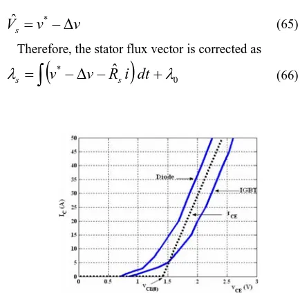
At very low speeds, the voltage drop in the PWM inverter can be higher than the induced voltage and, hence, constitutes a severe disturbance. In [25], the examination of this non-ideal effect and its compensation in an induction motor speed sensorless drive has been given. In this session, the effect of the forward voltage drop (FVD) in a SynRM drive will be analyzed. Fig. 5 shows the forward characteristics of the IGBT and diode used in this project. It is well known that the forward characteristics of the IGBT and its freewheeling diode are nonlinear, and they vary with temperature. However, according to their forward characteristic shown in Fig. 5 and datasheet, both can be represented by a DC voltage source and a resistance as given in (62). In order to simplify the analysis, it is assumed that the forward voltage drop of diode and IGBT are the same. The resistance term in (62) can be assumed as an extra stator resistance and therefore could be estimated by the stator
resistance estimator given in section V. In this section, the focus is to compensate for the error caused by
v
CE0.(62) CE
CE
CE
v
i
r
v
=
0−
The actual voltages with positive and negative currents are shown in Fig. 6. The left part of the figure is the inverter leg, the output voltage of which is either zero or
dc
V , ideally. The letter “s” in Fig. 6 shows the switching function of the inverter leg. Output voltage of the inverter leg with positive current (into the load) and negative current (from the load) are compared under the conditions of s=1 and s=0. It is seen that when the current is positive, the actual voltage is shifted down by vce, when the current is negative, the waveform of the actual output voltage of the inverter leg will shifted up by vce. After circuit analysis of the inverter, the error caused by the forward voltage drop of the switches of the inverter can be found. The error caused by FVD in one inverter leg is given in (63). Eq. (64) shows the error vector of the three phase inverter in the stationary frame.
(63)
( )
R CER DC
R s v v v sign i
v = * − = 0*
∆
and
(64)
( )
*( )
*( )
][ * 3
2 2
0 R S T
CE signi signi signi
v
v= +α +α
∆
where sign(.) is the signum function and
α
=
e
j2π/3.Using (64), an estimated value
V
ˆ
sof the stator voltagevector can be obtained from the SV-PWM reference
voltage vector
v
*described as follows(65)
v
v
V
ˆ
s=
*−
∆
Therefore, the stator flux vector is corrected as
(66)
(
)
0*
ˆ
λ
λ
s=
∫
v
−
∆
v
−
R
si
dt
+
Figure 5: Forward characteristics of the IGBT and diode of the Intelligent Power Model.
Figure 6: Analysis of the output voltage of an inverter leg.
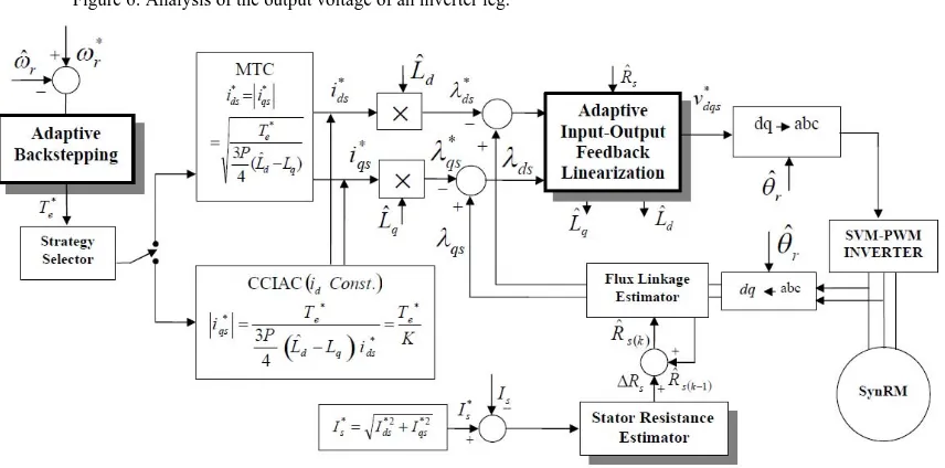
11. SIMULATIONRESULTS
The overall block diagram of the proposed drive system is shown in Fig. 7. Based on AIOFL, the motor supply voltage is synthesized from stator d and q axis
voltage commands (
v
*ds,
v
qs* ), using a two level spacevector modulation SVM-based PWM inverter. In addition, d and q axis stator fluxes are estimated by Eqs.
(1) and (2). A
C
++step by step computer program was developed to model the drive system control of Fig. 7. In this program, the system dynamic equations are solved by a static Range-Kutta fourth order method.In the proposed control approach the system controller gains are obtained by a trial and error method which are given by Kp=0.3 , KI=0.05 , γ =1 .5, γ =2 3,
225
1 2
α =α = and γ =.05. Assuming an exponential
speed reference from 0 to 1000 rpm with rise time
0.2 =
τ
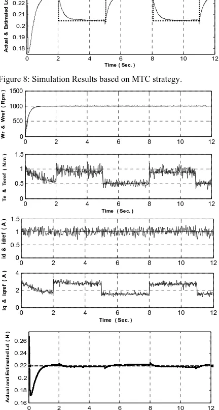
Sec., the simulation results are obtained forMTC and id constant strategies corresponding to a three-phase SynRM. The specifications and parameters of the three-phase SynRM used in our simulation program are given in Table 2. Simulation results obtained are shown in Figs. 8 and 9 in the case of J =2*Jm m,nominal, B=3*Bm,nominal.
As shown in these figures, the desired torque is stepped up and stepped down frequently. One can see that a perfect tracking control can be recognized for the two axis currents in spite of the parameters uncertainty and external load torque. The estimation errors in parameters Ld, Lq and Rs also converge to zero. It is worth mentioning that the torque ripples and motor two axis current harmonics seen in Figs. 8 and 9 can be explained by the effects of PWM inverter higher harmonics as well as by the higher harmonics induced in the SynRM rotor cage windings.
0 2 4 6 8 10 12 0
1 2
id
&
id
re
f
( A )
0 2 4 6 8 10 12
0 1 2
iq
&
iq
re
f
( A
)
0 2 4 6 8 10 12
0.18 0.19 0.2 0.21 0.22 0.23
Time ( Sec. )
A
c
tu
a
l
&
E
s
ti
m
a
te
d
L
d
( H
)
Figure 8: Simulation Results based on MTC strategy.
0 2 4 6 8 10 12
0 0.5 1 1.5
Time ( Sec. )
T
e
&
T
e
re
f (
N
.m
)
0 2 4 6 8 10 12
0 500 1000 1500
W
r
&
W
re
f
( Rp
m
)
0 2 4 6 8 10 12
0 0.5 1 1.5
id
&
id
re
f
( A
)
0 2 4 6 8 10 12
0 2 4
Time ( Sec. )
iq
&
iq
re
f
( A
)
0 2 4 6 8 10 12
0.16 0.18 0.2 0.22 0.24 0.26
Time ( Sec. )
A
c
tu
a
l
a
n
d
E
s
ti
m
a
te
d
L
d
( H
)
Figure 9: Simulation Results based on id Constant strategy.
12. EXPRIMENTAL SETUP AND RESULTS
A. Exprimental System Setup
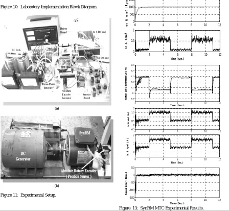
For practical evaluation of the actual system performance, a PC-based prototype system was built and tested. The experimental setup corresponding to the overall system block diagram shown in Fig. 7 is depicted in Figs. 10 and 11 consisting of the following parts: 1) A
0.37kW three-phase SynRM and a 1.1kW DC generator as its load, 2) a three-phase voltage source inverter and its isolation board, 3) voltage and current sensors board, 4) a 96 bit Advantech digital Input-Output card, 5) a 32-channel Advantech A/D converter card, 6) a CPLD board and a personal computer (PC) for calculating the required signals and viewing the registered waveforms. The 0.37kW SynRM parameters are reported in Table 2. The SynRM is supplied by a three-phase inverter with a symmetrical two level space vector modulation.
A Xilinx XC95288xl CPLD has been selected for real time implementation of switching patterns using a switching frequency of 5 kHz. The CPLD board communicates with PC via the digital Advantech PCI-1753 I/O board. CPLD in experimental setup realizes the following tasks:
1) Switching pattern generation of IGBT switches
based on the SVM technique providing a useful dead time in the so- called switching patterns of power switches.
2) generation of the synchronizing signal for data transmission between PC and hardware and
3) shutting down the inverter in the case of
emergency conditions such as over current or PC hanging states. The inverter has been designed and implemented specifically for this experiment using the SKM75 GD 124 D SEMIKRON module.
The required drive board has been designed by HCPL 316J which is fast and intelligent IGBT driver and guarantees a reliable isolation between the high voltage and the control boards. The DC link voltage and stator phase currents are measured by Hall-type LEM sensors. All measured electrical signals are filtered using the separate analogue second order low pass filters with 1.5 KHz bandwidth and then converted to digital signals using an A/D card with 10µsconversion time. In order to evaluate the accuracy of the rotor-speed and position estimation, the actual rotor position is obtained from an absolute encoder with 1024 pulses/r.
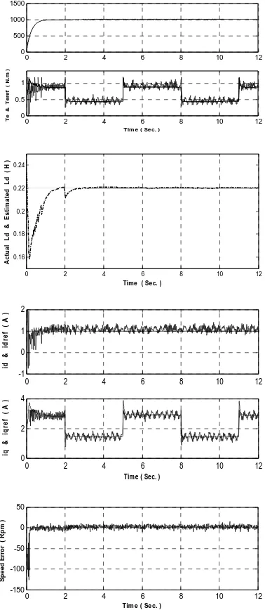
B. Experimental Results
Using the same conditions adopted to get SynRM simulation results as described in the previous section, the experimental results were obtained and shown in Figs. 13-15. It is seen that for the chosen id and iq reference currents, the estimated values of Ld and Lq approximately converge to these are obtained from Fig. 12 which shows the curves of Ld versus id and Lq versus iq obtained by the practical test.
almost a circle.
A close agreement is observed between simulation and practical results with a little disagreement, which may be because of inaccuracies that exist in our data acquisition system, SVPWM voltage source inverter effects and the dead times of inverter switching signals and also due to motor iron losses as well as ignoring the SynRM slotting torque effects that have not been taken into account in our system modeling.
Figure 10: Laboratory Implementation Block Diagram.
(a)
(b)
Figure 11: Experimental Setup.
0 0.5 1 1.5 2 2.5 3 3.5
0.16 0.18 0.2 0.22 0.24
id ( A )
A
c
tu
a
l
L
d
( H
)
Measured Fitted
0 0.5 1 1.5 2 2.5 3 3.5
0.1 0.11 0.12 0.13 0.14
iq ( A )
A
c
tu
a
l Lq (
H
)
Measured Fitted
Figure 12: Variations of d-axis inductance Ld with d-axis current id and q-axis inductanceLq with q-axis current iq.
0 2 4 6 8 10 12
0 500 1000 1500
wr
&
wr
e
f
(
R
p
m
)
0 2 4 6 8 10 12
0 0.5 1
Time ( Sec. )
Te
&
Te
re
f
0 2 4 6 8 10 12
0.19 0.2 0.21 0.22 0.23 0.24 0.25
Time ( Sec. )
A
c
tu
al
L
d
&
E
s
ti
m
a
te
d
Ld
(
H
)
0 2 4 6 8 10 12
-0.5 0 0.5 1 1.5 2
id
&
id
re
f (
A
)
0 2 4 6 8 10 12
0 1 2
Tim e ( Sec. )
iq
&
iq
re
f (
A
)
0 2 4 6 8 10 12
-150 -100 -50 0 50
Tim e ( Sec. )
Sp
e
e
d
Er
ro
r (
R
p
m
)
0 2 4 6 8 10 12 0
0.5 1
Tim e ( Sec. )
Te
&
Te
re
f
(
N
.m
)
0 2 4 6 8 10 12
0 500 1000 1500
0 2 4 6 8 10 12
0.16 0.18 0.2 0.22 0.24
Time ( Sec. )
A
c
tu
a
l L
d
&
E
s
ti
m
a
te
d
L
d
( H
)
0 2 4 6 8 10 12
-1 0 1 2
id
&
id
re
f
( A
)
0 2 4 6 8 10 12
0 2 4
Time ( Sec. )
iq
&
iq
re
f
( A
)
0 2 4 6 8 10 12
-150 -100 -50 0 50
Tim e ( Sec. )
Sp
e
e
d
Er
ro
r (
R
p
m
)
Figure 14: SynRM id Constant Strategy Experimental Results.
0 5 10 15 20 25
-20 0 20
wr
&
wr
e
f (
R
p
m
)
0 5 10 15 20 25
-20 0 20
Tim e ( Se c. )
S
p
e
e
d
E
s
ti
m
a
ti
o
n
E
rr
o
r
(R
p
m
)
Figure 15: Rotor low speed and position estimation.
TABLE 2
MOTOR NOMINAL CHARACTERISTICS
W
P
n=
37
0
V
n=
23
0
I
n=
2
.
8
A
, 232
md unSat
L = mH
L
md,Sat=
178
mH
L
mqn=
118
mH
Ω
=
2
.
95
snR
f
n=
6
0
Hz
No
.
of
Poles
=
4
m
N
T
en=
1
.
9
.
2Kg.m
015
.
=
mJ
B
m=
.
003
Nm/rad/sec
Web
Rateds,
=
.
5
λ
L
dr=
1
0
mH
L
qr=
8
mH
mH
13. CONCLUTION
In this paper, a method based on the adaptive input-output feedback linearization and adaptive backstepping
controller was designed for MTC and id constant
strategies of encoderless three-phase SynRM drive. The controller is capable of simultaneous estimation of direct and quadrature axis inductances. It has been shown that under Persistency of Excitation (PE) condition, the estimation errors in the motor d and q-axis inductances asymptotically converge to zero. The ABS speed controller was designed to compensate for the machine parameter uncertainties and load torque disturbances. Based on this control approach, the rotor low speed
estimation has been achieved by 1) using a simple method for eliminating the voltage sensors and a simple technique for online estimation of the stator resistance, and 2) taking into account the forward voltage drop of the inverter power switches. A close agreement was observed between simulation and practical results with a little disagreement due to 1) inaccuracies that exist in our data acquisition system, 2) SVPWM voltage source inverter effects, and the dead times of inverter switching signals, and 3) due to motor iron losses as well as ignoring the SynRM slotting torque effects that have not been taken into account in our system modeling.
14. REFERENCES
[1] R. Morales Caporal and M. Pacas, “A Predictive Torque Control for the Synchronous Reluctance Machine taking into account the magnetic cross saturation”, IEEE Trans. On Ind. Electronics, vol. 54, No. 2, pp. 1161-1167, Apr. 2007.
[2] T. H. Liu and H. H. Hsu, “Adaptive Controller Design for a Synchronous Reluctance Motor Drive System with Direct Torque Control”, IET Electric Power Appl., vol. 1, No.5, pp. 815–824 815, 2007.
[3] H.F. Hofmann, S.R. Sanders, and A. EL-Antably, “Stator-flux-oriented vector control of synchronous reluctance Machines with maximized efficiency”, IEEE Trans. On Industrial Electronics, vol. 51, Issue 5, pp. 1066-1072, Oct. 2004.
[4] H. D. Lee, S. J. Kang, and S. K. Sul, “Efficiency-Optimized DTC of Synchronous Reluctance Motor using Feedback Linearization”, IEEE Trans. On Ind. Elec., vol.46, No.1, pp. 192-198, 1999. [5] P. Guglielmi, M. Pastorelli and A. Vagati, ”Impact of
cross-saturation in sensorless control of transverse-laminated synchronous reluctance motors”, IEEE Trans. On Ind. Elect., vol. 53, Issue 2, , pp. 429-439, 2006.
[6] A. Vagati, M. Pastorelli, and G. Franceschini, “High-performance control of synchronous reluctance motors”, IEEE Trans. on Industry Appl., vol. 33, Issue 4, July-Aug. 1997, . pp. 983-991, 2004.
[7] E. M. Rashad, T. S. Radwan, and M. A. Rahman, “A MTPA Vector Control Strategy for Synchronous Reluctance Motors Considering Saturation and Iron Losses”, IEEE IAS, pp. 2411-2417, 2005. [8] M. G. Jovanovic, and R. E. Betz, “Optimal Torque Controller for
Synchronous Reluctance Motors”, IEEE Transactions on Energy Conversion, vol. 14, No. 4, pp. 1088-1093, December 1999. [9] R. E. Betz, R. Lagerquist, and M. Jovanovic, "Control of
Synchronous Reluctance Machies", IEEE Trans. On Industry Application, vol. 29, No. 6, pp. 1110-1122, Nov. 1993.
[10] S. Ichikawa, M. Tomita, S. Doki, and S. Okuma, "Sensorless Control of Synchronous Reluctance Motors Based on Extended EMF Models Considering Magnetic Saturation with Online Parameter Identification", IEEE Trans. On Industry Applications, vol. 42, No. 5, pp. 1264-1274, Sept./Oct. 2006.
[11] R. Marino, and P. Tomei, Nonlinear Control Design, Prentice Hall, Inc, 1995.
[12] R. Morales Caporal and M. Pacas, “Encoderless Predictive DTC for SynRM at Very Low and Zero Speed”, IEEE Trans. Ind. Elect., vol. 55, No. 12, pp. 4408-4416, Dec. 2008.
[13] C. A. M. D. Ferraz, and C. R. de Souza, ''Considering Iron Losses in Modeling the Reluctance Synchronous Motor'', 7th International workshop on Advance Motion Control (AMC), pp. 251-256, July 2002.
[14] H. Abootorabi Zarchi, J. Soltani and Gh. R. Arab Markadeh, ''Adaptive IOFL Based Torque Control of SynRM without Mechanical Sensor'', IEEE Trans. On Industrial Electronics, vol. 57, No. 1, pp. 375-384, January 2010.
[15] H. Abootorabi Zarchi, Gh. R. Arab Markadeh, and J. Soltani, ''Direct torque and flux regulation of synchronous reluctance motor
drives based on input–output feedback linearization'', Elsevier Journal, Energy Conversion and Management , vol. 51, pp. 71–80, January 2010.
[16] H. Abootorabi Zarchi, Gh. R. Arab Markadeh, and J. Soltani, ''Direct Torque Control of Synchronous Reluctance Motor using Feedback Linearization Including Saturation and Iron Losses', European Power Electronics and Drives (EPE) Journal, vol. 19,No.3, pp. 50-62, September 2009.
[17] L. Tang, and M. F Rahman, “Investigation of an Improved Flux Estimator of a Direct Torque Controlled Interior Permanent Magnet Synchronous Machine Drive”, 35th Annual IEEE Power Electronics Specialists Conf., Aachen, Germany, pp. 451-457, 2004.
[18] S. Mir, M.E Elbuluk, and D.S. Zinger, “PI and Fuzzy Estimators for Tuning the Stator Resistance in Indirect Torque Control of Induction Machines”, IEEE Tran. On Power Electronics, vol. 13, No. 2, pp. 279-287, March 1998.
[19] R. E. Betz, ''Theoretical Aspects of the Control of Synchronous Reluctance Machines'', IEE Proceeding B, vol. 139, No. 4, pp. 355-364, July 1992.
[20] R. E. Betz, and T. J. E., Miller, ''Aspects of the Control of Synchronous Reluctance Machines", Proceedings European Power Elect. Conf., pp. 456-463, EPE 1991.
[21] A. Chiba, and T. Fukao, ''A Closed-loop Operation of Super High-Speed Reluctance Motor for Quick Torque Response'', IEEE Trans. On Industry Applications, vol. 28, No. 3, pp. 600-606, 1992. [22] T. A. Lipo, ''Synchronous Reluctance Machines- A viable
alternative for ac drives'', Electric Machines and Power Systems, vol. 19, pp. 659-671, 1991.
[23] J. Holtz, and J. Quan, “Drift- and Parameter-Compensated Flux Estimator for Persistent Zero-Stator-Frequency Operation of Sensorless-Controlled Induction Motors”, IEEE Trans. On Ind. Appl., vol. 39, No. 4, pp. 1052-1060 , July/Aug. 2003.
[24] V. d. Broeck, H. C. Skudelny, and G. V. Stanke, “Analysis and Realization of a Pulse Width Modulator Based on Voltage Space Vectors”, IEEE Trans. On Ind. Appl., vol. 24, No. 11, pp. 142-150, 1988.
[25] J. Holtz, “Sensorless Control of Induction Machines -With or Without Signal Injection?”, IEEE Trans. On Ind. Elect. , vol. 53, No. 1, pp. 7-30, Feb. 2006.