Direct Torque Control with Sliding mode Feedback Linearization for SVM Inverter Fed Induction Motor Drives

(1)

IJSRSET1738127 | Received : 15 Nov 2017 | Accepted : 05 Dec 2017 | November-December-2017 [(3)8: 415-424]

415

Direct Torque Control with Sliding mode Feedback

Linearization for SVM Inverter Fed Induction Motor Drives

D. Mastan*

1

, S. Sridhar

2

, B. Naresh

3

*1_{M.Tech student, Electrical Engineering, JNTUA College of Engineering, Anantapuramu, Andhra Pradesh, India}

2_{Asst. Professor, Electrical Engineering, JNTUA College of Engineering, Anantapuramu, Andhra Pradesh, India}

3_{Asst. Professor, UCEK, JNTU Kakiada , Andhra Pradesh, India}

ABSTRACT

This paper presents a feedback linearization Direct Torque Control (DTC) based on space vector modulation (SVM) which can be noticeably reduce electromagnetic torque and stator flux ripples that affect Induction Motor (IM) drive. In this paper IM drive that utilizes feedback linearization, Sliding-Mode Control (SMC) and a Fuzzy logic speed controller is discussed. A modern feedback linearization approach is proposed, which gives a decoupled direct IM model with two state variables: torque and stator flux magnitude. This obtained linear model is utilized to implement a DTC type controller that maintains all DTC advantages and suppresses its main drawback, the flux and torque ripple. Robust, quick, and ripple free control is accomplished by utilizing SMC with proportional component in the region surrounded by the sliding surface. SMC ensures robustness as in DTC, while the proportional component wipes out the torque and flux ripple. The torque time response is similar to traditional DTC and the proposed solution is able to adjust, profoundly tunable because of the P component. The sliding controller is compared with linear DTC scheme with and without feedback linearization. The conventional scheme uses proportional integral controller to achieve speed control. The fuzzy logic controller replaces the PI speed controller in the proposed scheme to ensure fast speed response in the drive. The extensive simulation results are presented and compared with the conventional scheme.

Keywords : Direct torque control, adjustable speed drives, feedback linearization, induction motor drives, sliding mode control, fuzzy logic controller

I. INTRODUCTION

The basic concept of Direct Torque Control (DTC) of Induction Motor (IM) drives is to control both the stator flux magnitude and electromagnetic torque of machine simultaneously. DTC provides lower parameter sensitivity and fast dynamic response, when compared with conventional vector controlled IM drives [1],[2]. DTC was recognized as a viable alternative to Field oriented control (FOC), being also general philosophy for controlling the adjustable speed drives (ASD). DTC has structural simplicity, abandons the stator current control philosophy, characteristic of FOC and achieves hysteresis torque and flux control by directly modifying the stator voltage in accordance with the torque and flux errors. The classic DTC consists of the bang-bang or closed loop hysteresis control of torque and flux

(2)

Recently, the nonlinear control technique based on the feedback linearization (FBL) theory has been used for various applications in the area of power electronics and drives. A high performance Feedback linearization control system for SVM inverter fed IM drive is presented. FBL is sensitive to modeling errors and disturbances. Despite its usefulness, the FBL has been rarely applied to IM drives. FBL is utilized in [6]-[10] to linearize the IM model with regard to speed, flux, and current. Two linearization methods in which only one control quantity is transformed are discussed in [12]. All solutions in [6]-[10] are depending on current linearization and control. Applications of FBL to power electronics and PMSM drives are discussed in [11]-[14]. An error sensitivity analysis in [8] reveals that the control performance may deviate due to perturbations, parameter detuning and measurement errors.

The Sliding Mode Controller (SMC) technique is applied to the resulting linear system obtained by feedback linearization. SMC is a robust control technique well suitable for control systems with uncertainties or modeling errors [15]. The robustness and the discontinuous nature of variable structure control allows to SMC controller to the SVM fed IM drives. It has been effectively applied to IM drives and provides superior dynamic performance for a wide range of operation [5], [7],[14]-[18]. The basic theory behind the SMC is that the system structure is switched when the system state crosses the predetermined discontinuity line, so that the state slides along the reference trajectory. The switching pattern can be applied with the VSI operation as in [15]. In fact, the traditional DTC is a form of SMC which was designed to closely match the switching nature of the VSI.

Therefore, this paper proposes a feedback linearization direct torque control technique based on SVM to remarkably reduce the electromagnetic torque and stator flux magnitude ripples for IM drives. To apply the proposed DTC strategy, the decoupled dynamic model of IM is first introduced by defining two states (i.e., the stator flux and torque). Next, feedback linearization (FBL) is applied to IM model for obtaining an equivalent linearized model, and then utilizing the sliding mode controller (SMC) technique. The main advantage of FBL when compared to classic DTC is that linear control theory can easily be applied to obtain better performance. We use this property to design and

theoretically investigate the robustness and stability of the proposed control method. The main disadvantage of FBL is the sensitivity of the linearized model to uncertainties and parameter detuning which motivates the inclusion of the SMC.

The nonlinear IM model treated in this paper is fourth order with the state variables: torque, stator flux, rotor flux and other flux-dependent state. The obtained linear IM model using FBL is of second order, with only the torque and stator flux magnitude as dissociate state variables. Thus the new linear IM model is obtained spontaneously, very simple, and it substantially simplifies the controller design. The flux and torque are controlled by the new DTC scheme and the proposed controllers include SMC to maintain robust sensorless operation of IM drive. This technique based on the torque-flux linearization and control is different from existing methods discussed in [6]-[8], which are depending on current control. The combination of FBL and SMC techniques preserves the fast and robust response of conventional DTC while entirely eliminating the torque and flux ripple.

II. IM Model Using FEEDBACK

LINEARIZATION

(3)

The IM state space model in the stator reference frame is

𝑡 𝑇 𝑇

𝑢 ( )

𝑡 𝑇

(

𝑇 ) ( )

where s, r are stator and rotor flux space vectors, Rs

and Rr are the stator and rotor resistances, Ls, Lr and

Lm are the stator, rotor and magnetizing inductances, 𝑇𝑠

= 𝑠 /𝑅𝑠, 𝑇𝑟 = 𝑟 /𝑅𝑟 , = ( 𝑠 𝑟 – 𝑚2_{)/ 𝑠 𝑟}_,r _is

the rotor speed, and 𝑢𝑠 = 𝑢𝑠 + 𝑢𝑠𝑞 is the stator voltage vector which acts as input.

The model can be linearized by selecting the new states:

𝑀 = 𝑠𝑞 𝑟 – 𝑠 𝑟𝑞 (3)

𝑅 = 𝑠 𝑟 + 𝑠𝑞 𝑟𝑞 (4)

𝐹𝑠 = 𝑠 2 + 𝑠𝑞2 (5)

𝐹r = 𝑟 2 + 𝑟𝑞2

(6)

Where 𝑀 is the scaled torque, Fs and Fr are the squared magnitudes of the stator and rotor flux, respectively. The variable 𝑅 relies upon the rotor and stator flux. We refer M as the torque and Fs as the flux magnitude. We are essentially keen on controlling the torque 𝑀 and the stator flux magnitude 𝐹𝑠. In any case, we should insure

that remaining state factors, Fr and R, are limited. The IM state equations with the state factors (3) - (6) are

( + )𝑀 𝑟𝑅 𝑟𝑞𝑢𝑠 + 𝑟 𝑢𝑠𝑞 (7)

𝐹𝑠+

𝑅+2 𝑠 𝑢𝑠 +2 𝑠𝑞𝑢𝑠𝑞 (8)

𝐹

_𝑅

(9)

( + )𝑅+ 𝑟𝑀+ 𝐹𝑠+

𝐹𝑟+ 𝑟 𝑢𝑠 + 𝑟𝑞

𝑢𝑠𝑞 (10)

The first three state equations are feedback linearized if the inputs redefined as

𝑤𝑞 𝑟𝑅 𝑟𝑞 𝑢𝑠 + 𝑟 𝑢𝑠𝑞 (11)

𝑤 = 𝑅 + 2( 𝑠 𝑢𝑠 + 𝑠𝑞 𝑢sq) (12)

Now the linearized system is

( + ) 𝑀 +wq

(13)

𝐹𝑠 +wd (14)

𝐹

𝑅 (15)

( + ) 𝑅 +

𝐹𝑠 + wd-- wq (16)

Solving (11) and (12) gives the control signals usd= (𝑤 )

₍ _{𝑅) ( )}

usq=

(𝑤

)

₍ _{𝑅) ( )}

FBL decouples the state factors of interest; specifically, the torque 𝑀 and the stator flux magnitude 𝐹𝑠 and thus

substantially, make easier the controller design for the IM drive system. Further, the resulting system is linear, the traditional linear control approaches can be utilized. Since the 𝑀, 𝐹𝑠 and 𝐹𝑟 have dynamics with left plane

poles, the input output stability of the remaining of the state factors can be effortlessly ensured that 𝑅 remains limited. The R state equation (16) demonstrates that its right hand side is unbounded for zero 𝑅, which just happens in the trivial condition when the stator or rotor flux is zero. With the exception for the startup, this condition never happens during normal operation. Simulation results demonstrate that the torque control has begun with a 40 ms delay after the flux control, when fluxes are at ostensible levels. It is therefore accepted that the variable 𝑅 has a lower bound, 𝑅l. 𝑅 is

also upper limited because that the flux magnitudes are

restricted due to magnetic saturation.

III. DIRECT TORQUE CONTROL VIA SLIDING

MODE

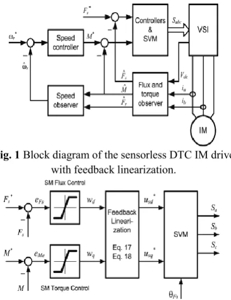
Sliding Mode Control (SMC) is utilized to accomplish a quick and strong operation of an IM drive. Fig. 1 demonstrates the block diagram of the proposed drive. The block Controllers and SVM contains the FBL and the torque and flux controllers described next. The drive utilizes speed, torque, and flux observers, a fuzzy logic speed controller.

The control objective is to control the torque 𝑀

and stator flux magnitude 𝐹𝑠 in the machine, i.e. to

actualize a DTC type controller. To this end, we design controllers for the torque 𝑀, and the stator flux 𝐹𝑠 in the

linearized model. Since the state equations (13) and (14) representing 𝑀 and 𝐹𝑠 individually are decoupled, the

(4)

and 𝑤𝑞 is simple. These are then substituted in (17) and

(18) to acquire the physical inputs 𝑢𝑠 and 𝑢𝑠𝑞 separately.

However, errors in the computation of the physical inputs are unavoidable and must be evaluated and corrected to give robust performance.

Fig. 1 Block diagram of the sensorless DTC IM drive with feedback linearization.

Fig. 2 Torque and flux SMC with feedback linearization for IM control.

The errors in the physical control inputs can be serve as proportionate errors in the linear state equations (13) and (14).

Equation (13) can be modified in the form

𝑔M+wq (19)

where 𝑔M represents the uncertain dynamics of the FBL

torque equation. The term 𝑔𝑀 is not exactly known; from (13) an approximate of the dynamics is

𝑔̂M= ( ) 𝑀.

We assume that the estimate error for 𝑔𝑀 is bounded as

|𝑔 𝑀 𝑔𝑀| ≤ 𝐺𝑀

(20)

To design the SMC for the linear system of (19), we define the sliding surface as the torque error

𝑆𝑀 = 𝑀 𝑀 (21)

For this selection of sliding surface, we use the SMC

𝑤𝑞 𝑔 𝑀 – 𝑘𝑀sgn(𝑆𝑀) , 𝑘𝑀 > 0 (22)

The term 𝑘𝑀sgn(𝑆𝑀) is known as the corrective

control.

We take the quadratic Lyapunov function prospect 𝑉= 𝑆M2/2. The system converges to the sliding surface if

the derivative of a Lyapunov function is negative with all the trajectories of the system. The derivative of V is

𝑆𝑀2=(𝑔𝑀 𝑔 𝑀 𝑘𝑀sgn(𝑆𝑀))𝑆𝑀 = (𝑔𝑀 𝑔 𝑀)𝑆𝑀

𝑘𝑀|𝑆𝑀|

(23)

For robust convergence to the sliding surface the derivative must remain negative in the presence of uncertainties. We choose the corrective control gain 𝑘𝑀

as in eq. (24).

𝑘𝑀 = 𝐺𝑀 + 𝜂𝑀 (24)

This gives the sliding condition, eq. (25)

𝑆𝑀2≤ 𝜂𝑀|𝑆𝑀| (25)

where 𝜂𝑀 is a positive constant. The gain 𝑘𝑀 of (24)

includes the term 𝐺𝑀 to ensure robust stability and the

term 𝜂𝑀 to control the speed of convergence to the

sliding controller. A larger 𝜂𝑀 makes the system

trajectory to get the sliding surface in a shorter time but can result in larger chattering. Similar results can be obtained by utilizing an integral sliding surface

𝑆𝑀 = (+ 𝜆𝑀) ∫ ( ) (26)

where 𝜆𝑀 is a positive constant design parameter. This parameter regulates how fast the error goes to zero once the state is on the surface. The SMC effort can be chosen as

𝑤𝑞 𝑔 𝑀 ( ) 𝑘𝑀sgn(𝑆𝑀) , 𝑘𝑀 > 0 (27)

and the sliding condition take hold for 𝑘𝑀 = 𝐺𝑀 + 𝜂𝑀.

To limit chattering we specify a boundary layer around the sliding surface, BM(𝑡) = {𝑥, |(𝑥)| ≤ ℎM}, where ℎ𝑀 > 0 is the boundary layer thickness. Inside the boundary layer, a proportional control term is added to the control of (22). Outside the boundary layer (𝑆𝑀|(𝑥)| > ℎ𝑀), the

corrective control drives the system to the sliding surface.

The stator flux dynamics in eq. (14) are similar to (13) and are similarly handled. Most of the analysis is excluded, for brevity. Similar to torque, the sliding surface for stator flux is

𝑆𝐹𝑠 = 𝐹𝑠 𝐹𝑠 (28)

and the linear system control feedback is

𝑤 𝑔 𝐹𝑠 𝑘𝐹𝑠 sgn(𝑆𝐹𝑠 ) , 𝑘𝐹𝑠 > 0

(5)

As for torque, we use a thin boundary layer around the sliding surface, with proportional control to omit chattering. Figure 2 shows the block diagram of the SMC with FBL torque and flux controller. To summarize, the controllers are given by (22) and (29) and the reference voltages are produced by (17) and (18) in the stator reference frame. A SVM unit produces the VSI switching signals Sa, Sb, Sc.

IV. CONTROLLER DESIGN AND ROBUSTNESS

STUDY

This segment gives a design procedure to the sliding mode FBL controller that accomplishes robust stability in terms of the most important errors which influence the IM model: motor parameter detuning and speed observation errors. We consider these vulnerabilities limited, as in eq. (20) and enquire how these vulnerabilities affect the selection of corrective gains for torque and flux control. For FBL performance we utilize consistent motor parameter values and design the controller to maintain robustness as they vary during operation. Rotor speed can get from observers with estimation errors, especially during transients and low speed operation. Then again, flux and torque observers give moderately good estimations, and the impact of their errors on FBL is not considered here.

The errors in the control signal because of these vulnerabilities are represented as Δ𝑢𝑠 and Δ𝑢𝑠q. To

assess these errors in terms of the rotor speed and parameter errors and to analyze the impact of vulnerabilities on the SMC design we consolidate (17) and (18) in vector form:

𝑢𝑠=( ) +j(wq/R+ r) (30)

Although 𝑤 and 𝑤𝑞 are generated by the SMC and have no uncertainty, we can replace the error in the control signal us with equivalent errors in 𝑤 and 𝑤q. The equivalent error is Δ𝑤 Δ𝑤 + Δ 𝑤q, and (30) can be modified as (31).

𝑢𝑠=(

̂ ̂

( ̂ )( ̂ ) ) +j(

+ r)

(31)

where 𝑚 is the measured magnetizing inductance,

𝑅 𝑠 is measured stator resistance and 𝑟 is the rotor

speed estimate.

Using (30) and (31), the equivalent error is (32).

Δ𝑤 Δ𝑤 + Δ𝑤𝑞 =

2(₍_̂ ̂ ̂

)( ̂ )

)R+j( r - ̂r)R (32)

The feedback linearized torque and stator flux dynamics in the presence of errors in 𝑤 and 𝑤𝑞are

( ) 𝑀+wq Δ𝑤𝑞 (33)

𝐹𝑠 +wd Δ𝑤 (34)

It can be assumed that the maximum deviation of each uncertain parameter and the maximum measurement or estimation error for the rotor speed are known. For this analysis we use 𝜂𝑀 = 10, 𝜂𝐹𝑠 = 10, which give a

realistic dynamic response for torque and flux. The main focus for this section is robust stability rather than dynamic response.

A. Speed ( 𝑟)

Errors in speed estimation create model perturbations that may affect the system response. Speed errors have no impact on stator flux dynamics but change the torque equation (13) to

( ) 𝑀 (̂ r)R+wq (35)

Knowing the maximum speed estimation error, the corrective control gain can assures robust performance. The IM has a nominal value of R, R = 0.25. Assuming a speed measurement with a maximum error of ±10 rad/s (±1.6 Hz), we have |( 𝑟 𝑟 )𝑅| < 2.5,which relates

to 𝐺𝑀 = 2.5 and 𝑘𝑀 = 𝐺𝑀 + 𝜂𝑀 = 12.5. We use 𝑘𝑀 =

20, as in our simulations, which handles even larger errors. Since the speed error does not affect the stator flux dynamics, we use 𝑘𝐹𝑠 = 𝜂𝐹𝑠 + 0 = 10.

Simulation results in Fig. 10,11 show the torque and flux response for the drive starting from standstill with ±10 rad/s speed errors. The torque control is almost similar for any speed error and it remains stable and ripple-free. For larger errors we simply choose a higher gain for robust stability, at the expense of increased chattering.

(6)

The stator resistance changes with temperature, and it influences the stator flux dynamics. Introducing a perturbation because of stator resistance error, the stator flux dynamics (34) is

𝐹𝑠 +

𝑅(𝑅 𝑅̂)wd (36)

where𝑅 𝑠 is the nominal stator resistance and 𝑅𝑠 is its original value. We consider a maximum error in the stator resistance of 50%, i.e. |𝑅𝑠 𝑅 𝑠| < 0.5 ×𝑅 𝑠 = 1.15. The corresponding model perturbation for the parameter values is 𝐺𝐹𝑠 = 𝑅×0.69 = 28.16. We select the corrective control gain 𝑘𝐹𝑠 =𝜂𝐹𝑠 + 𝐺𝐹𝑠 =

40>38.16. Since the torque dynamics independent of

the resistance error, we use the same value 𝑘𝑀=20, for

similar dynamic performance.

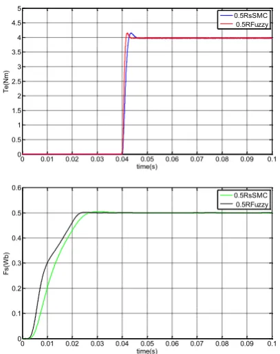
Simulation results in Fig. 8,9 show the stator flux and torque response for the drive starting from standstill with 50% stator resistance dynamic uncertainty. Observe how the resistance error affects the flux response time, which is faster for lower resistances and due to larger gain. However, the steady state operation is ripple-free and robust with respect to Rs errors.

C. Rotor resistance (𝑅𝑟)

Rotor resistance varies with temperature. The notable advantage of the proposed FBL is that the changes in Rr do not vary the dynamics of stator flux and torque and do not affect the control. However, they do change the dynamics of the other two state variables (𝑅, 𝐹𝑟); this substantially affects the speed estimate. Therefore, the rotor resistance errors are accounted for by speed errors discussed in section IV.A.

D. Magnetizing inductance ( 𝑚)

The magnetizing inductance deviates from its measured value due to magnetic saturation. Changes in the magnetizing inductance produce changes in both the stator and rotor inductances. This has no impact on torque dynamics, but alters the stator flux dynamics (34), as follows:

𝐹𝑠+

𝑅 (

̂

( ̂ )( ̂ ) ) wd

(37)

We consider a maximum change in the magnetizing inductance of 30%, i.e. 0.7 𝑚 𝑚1.3 𝑚. We

examine the term  = ₍_̂ ̂

)( ̂ )

in (37) that depends on 𝑚. For 𝑚 = 0.7 𝑚 we have

 0.4 46 , and for 𝑚 = 1.3 𝑚 we have  =

0.23176. For robust stability we use the maximum

value of | |. The corresponding perturbation is 𝐺𝐹𝑠 =

2𝑅𝑅𝑠 × 0.42467 = 0.49. We use the gain 𝑘𝐹𝑠 = 12 >

10.49. Since the torque dynamics is independent of the

magnetizing inductance, we use 𝑘𝑀 =20. Simulation

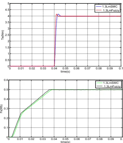
results in Fig. 6,7 show the stator flux and torque for the drive starting from standstill with 30% magnetizing inductance errors. Again, it is proved that SMC provides robust and ripple-free steady state performance. Overall, the largest gains can be used for all situations. All simulations are for the sensorless drive shown in Fig. 1.

The proposed SMC design is based on the required dynamic response (𝜂𝑀, 𝜂𝐹𝑠) and the maximum

uncertainty (𝐺𝑀, 𝐺𝐹𝑠).The dynamic response is

application-dependent and is chosen by the designer. Equation (34) gives the maximum uncertainty caused by FBL. Given 𝜂 and 𝐺 for flux and torque, the designer chooses a sliding gain larger than 𝐺𝑀 + 𝜂𝑀 for the

torque controller and larger than 𝐺𝐹𝑠 + 𝜂𝐹𝑠 for the flux

controller. This selection of the corrective control gains results in a robust and stable system that operates at the required speed while suppressing chattering. Comparing all simulation results, we conclude that larger gains result in a faster and robust control, but can cause chattering if the increase in gain is excessive.

V. Fuzzy Logic Controller

Usage of conventional control "PI", its response is not all that great for non-linear systems. The change is noticeable when controls with Fuzzy logic are utilized, acquiring a superior dynamic response from the system. Fuzzy Logic Controller (FLC) has been presented and been utilized. The benefits of fuzzy logic controllers over traditional PI controllers are that they needn't bother with a precise scientific model, Can work with uncertain information sources and can deal with nonlinearities and are more powerful than traditional PI controllers. The fuzzy rule base used in this paper is

e

NH NM NS ZE P H

PM PS

NH NH NH NH NH P

M

PM ZE

NM NH NH NH N

M

(7)

NS NH NH N M

NS ZE PS PM

ZE NH NM NS ZE PS PM PH

PH NM NS ZE ZE P

M

PH PH

PM NS ZE NS PM PH PH PH

PS ZE NS N M

PH PH PH PH

Table 1: Fuzzy rule base

Fig 3: Membership functions for input 1

Fig 4: Membership functions for input 2

Fig 5: Membership functions for output

V. Comparison of DTC Schemes

Controller Rise

time

Settling time

PI without FBL 3.5ms 5ms

PI with FBL 1.7ms 3ms

SMC with FBL 1.2ms 1.5ms

Fuzzy with SMC & FBL

0.99ms 1.1ms

Tab 2: Comparison of various DTC schemes

VI. SIMULATION RESULTS

Fig 6: Simulation results for SMC and FBL for existed and proposed with +30% Lm errors, at startup, torque Te,

and stator flux

Fig 7: Simulation results for SMC and FBL for proposed and extinction with -30% Lm errors, at startup,

torque Te, and stator flux 𝑠.

0 0.01 0.02 0.03 0.04 0.05 0.06 0.07 0.08 0.09 0.1 0

0.5 1 1.5 2 2.5 3 3.5 4 4.5 5

Te

(N

m

)

time(s)

1.3LmSMC 1.3LmFuzzy

0 0.01 0.02 0.03 0.04 0.05 0.06 0.07 0.08 0.09 0.1 0

0.1 0.2 0.3 0.4 0.5 0.6

Fs(

W

b)

time(s)

1.3LmSMC 1.3LmFuzzy

0 0.01 0.02 0.03 0.04 0.05 0.06 0.07 0.08 0.09 0.1 0

0.5 1 1.5 2 2.5 3 3.5 4 4.5 5

T

e(

N

m

)

time(s)

0.7LmSMC 0.7LmFuzzy

0 0.01 0.02 0.03 0.04 0.05 0.06 0.07 0.08 0.09 0.1 0

0.1 0.2 0.3 0.4 0.5 0.6

F

s(

W

b)

time(s)

0.7LmSMC 0.7LmFuzzy

0 0.01 0.02 0.03 0.04 0.05 0.06 0.07 0.08 0.09 0.1 0

0.5 1 1.5 2 2.5 3 3.5 4 4.5 5

Te

(N

m

)

time(s)

(8)

Fig 8: Simulation results for SMC and FBL for existing and proposed models with +50% Rs errors, at startup,

Fig 9: Simulation results for SMC and FBL for existing and proposed models with -50% Rs errors, at startup,

Fig 10: Simulation results for SMC and FBL for existing and proposed model with -10 rad/s speed errors,

at startup, torque Te s.

Fig 11: Simulation results for SMC and FBL for exising and proposed model with +10 rad/s speed errors, at

startup, torque Te, and stator flux 𝑠.

a)Torque response to 4.5 Nm step command with Linear DTC and

without FBL

0 0.01 0.02 0.03 0.04 0.05 0.06 0.07 0.08 0.09 0.1 0

0.1 0.2 0.3 0.4 0.5

F

s

(

Wb

)

Time(s)

1.5RsSMC 1.5RsFuzzy

0 0.01 0.02 0.03 0.04 0.05 0.06 0.07 0.08 0.09 0.1 0

0.5 1 1.5 2 2.5 3 3.5 4 4.5 5

T

e(

N

m

)

time(s)

0.5RsSMC 0.5RFuzzy

0 0.01 0.02 0.03 0.04 0.05 0.06 0.07 0.08 0.09 0.1 0

0.1 0.2 0.3 0.4 0.5 0.6

F

s(

W

b)

time(s)

0.5RsSMC 0.5RFuzzy

0 0.01 0.02 0.03 0.04 0.05 0.06 0.07 0.08 0.09 0.1 0

0.5 1 1.5 2 2.5 3 3.5 4 4.5 5

T

e

(N

m

)

time(s)

-10%SMC -10%Fuzzy

0 0.01 0.02 0.03 0.04 0.05 0.06 0.07 0.08 0.09 0.1 0

0.1 0.2 0.3 0.4 0.5 0.6

F

s(

W

b)

time(s)

-10%SMC -10%Fuzzy

0 0.01 0.02 0.03 0.04 0.05 0.06 0.07 0.08 0.09 0.1 0

0.5 1 1.5 2 2.5 3 3.5 4 4.5 5

T

e(

N

m

)

time(s)

+10%SMc +10%Fuzzy

0 0.01 0.02 0.03 0.04 0.05 0.06 0.07 0.08 0.09 0.1

0 0.1 0.2 0.3 0.4 0.5 0.6

F

s(

W

b

)

time(s)

+10%SMc +10%Fuzzy

0 0.005 0.01 0.015 0.02 0.025

-1 0 1 2 3 4 5

Time(s)

T

e

(N

m

)

(9)

b)Torque response to 4.5 Nm step command with Linear DTC and with FBL

Fig 12: Torque response to 4.5 Nm step command for (a) PI controllers (Linear DTC) and (b) PI controllers

and FBL. Startup from standstill.

a)Stator (blue) and rotor (green) flux magnitude control at startup with Linear DTC and without FBL

b)Stator (blue) and rotor (green) flux magnitude control at startup with Linear DTC and with FBL

Fig 13: Stator (blue) and rotor (red) flux magnitude control at startup, for proposed and extinction with (a) PI controllers (Linear DTC) and (b) PI controllers and

FBL.

a)Torque response to 4.5 Nm step command with feedback linearization and SMC

b)Stator (blue) and rotor (green) flux magnitude control at startup with feedback linearization and SMC

Fig 14: Torque transients for startup from standstill with feedback linearization and SMC (a) torque, (b) stator

and rotor flux magnitudes.

a)Torque response to 4.5 Nm step command for Fuzzy logic Controller with SMC and FBL

b)Stator (blue) and rotor (green) flux magnitude control at startup with Fuzzy Logic Controller

Fig 15: Stator (blue) and rotor (red) flux magnitude response to 0.5 Wb step command for fuzzy logic controller with feedback linearization and SMC, at

standstill.

VII. CONCLUSION

This paper describes a modern approach which incorporates Feedback linearization and sliding mode control with fuzzy logic controller for a DTC drive. This new arrangement based on torque-flux linearization creates an instinctive linear model of the IM, with electromagnetic torque and flux as decoupled state

0 0.005 0.01 0.015 0.02 0.025

-1 0 1 2 3 4 5

Time(s)

T

e

(N

m

)

Electromagnetic Torque

0 0.01 0.02 0.03 0.04 0.05 0.06 0.07 0.08 0.09 0.1 -0.1

0 0.1 0.2 0.3 0.4 0.5 0.6

Time

St

at

or

fl

ux

0 0.01 0.02 0.03 0.04 0.05 0.06 0.07 0.08 0.09 0.1 -0.1

0 0.1 0.2 0.3 0.4 0.5 0.6

Time

S

ta

to

r

F

lu

x

0 0.005 0.01 0.015 0.02 0.025

-1 0 1 2 3 4 5

Time

T

e

(N

m

)

0.050 0.055 0.06 0.065 0.07 0.075 0.08 0.085 0.09 0.095 0.1 0.1

0.2 0.3 0.4 0.5 0.6

Time

S

ta

to

r

flu

x

0 0.005 0.01 0.015 0.02 0.025

-1 0 1 2 3 4 5

Time(s)

T

e

(N

-m

)

0.050 0.055 0.06 0.065 0.07 0.075 0.08 0.085 0.09 0.095 0.1

0.1 0.2 0.3 0.4 0.5 0.6

Time

S

ta

to

r

F

lu

(10)

factors. The proposed fuzzy logic controller with SMC and FBL has been simulated, with a simple torque and flux observer which produces finest results. The torque response is very fast and chattering free with low steady state ripple.

Despite the simple torque, flux and speed observer and other errors, the speed control is fast and accurate. For the linear IM model, the controller-observer principles shall be designed independently, if estimation errors are small. It also allows the utilization of conventional linear design approach and linear state observers.

Direct torque and flux control gives robustness against parameter vulnerabilities when sliding mode controller is used, as demonstrated by the correlation with a linear controller. The chattering related with sliding mode operation is suppressed by the proportional controller utilized inside the boundary layer. The drive has a similar quick and robust response, as a regular DTC drive and totally suppressed the torque and flux ripple. Finally the new arrangement consolidates the benefits of conventional and linear DTC. These achievements are because of the sliding mode controller and the linearization which decouples the torque and stator flux extent. Extensive simulation results carried out demonstrate that torque-flux feedback linearization is a helpful technique to deal with IM drive speed control. It permits independent design of controllers and observers, and helps in the integration of conventional linear and nonlinear controllers.

VIII. REFERENCES

[1]. G. Buja, M.P. Kazmierkowski, “Direct torque control of PWM inverter-feed ac motors – A survey,” IEEE Trans. Industrial Electronics, vol. 51, no. 4, Aug. 2004, pp. 744-757

[2]. I. Takahashi, T. Noguchi, “A New Quick Response and High Efficiency Control Strategy of an Induction Motor,” Rec. IEEE IAS,1985 Annual Meeting, pp. 495-502, 1995.

[3]. Y.-S. Lai, W.-K. Wang, Y-C. Chen, “Novel switching techniques for reducing the speed ripple of ac drives with direct torque control,” IEEETrans. Industrial Electronics, vol. 51, no. 4, Aug. 2004, pp. 768-775.

[4]. C. Lascu, A.M. Trzynadlowski, “A sensorless hybrid DTC drive for high volume low-cost applications,” IEEE Trans. Industrial Electronics, vol.51, no. 5, Oct. 2004, pp. 1048-1055.

[5]. C. Lascu, I. Boldea, F. Blaabjerg, “Variable-Structure Direct Torque Control – A Class of Fast and Robust Controllers for Induction Machine Drives,” IEEE Trans. Industrial Electronics, vol. 51, no. 4, Aug. 2004, pp.785-792.

[6]. M.P. Kazmierkowski, D. Sobczuk, “High performance induction motor control via feedback linearization,” Proc. IEEE ISIE’95, vol. 2, pp.633-638, July 1995.

[7]. M.P. Kazmierkowski, D. Sobczuk, “Sliding mode feedback linearization of PWM inverter fed induction motor,” Proc. IEEEIECON 1996, vol. 1, pp, 244-249, Aug. 1996.

[8]. T.K. Boukas, T.G. Habetler, “High-performance induction motor speed control using exact feedback linearization with state and state derivative feedback,” IEEE Trans. Power Electronics, vol. 19, no. 4,July 2004, pp. 1022-1028.

[9]. John Chiasson, Modeling and high-performance control of electric machines, John Wiley and Sons Inc., 2005.

[10]. J. Chiasson “A new approach to dynamic feedback linearization control of an induction motor,” IEEE Trans. Automatic Control, vol. 43, no. 3,Mar 1998, pp. 391-397.

[11]. Y.S. Choi, H.H. Choi, J.W. Jung, “Feedback linearization direct torque control with reduced torque and flux ripples for IPMSM drives,” IEEE Trans. Power Electronics, vol. 31, no. 5, May 2016, pp. 3728-3737.

[12]. P. Liutanakul, S. Pierfederici, F.M. Tabar, “Application of SMC with I/O feedback linearization to the control of the cascade controlled rectifier/inverter-motor drive system with small dc link capacitor,” IEEE Trans. Power Electron., vol. 23, no. 5, Oct 2008, pp. 2489-2499.

[13]. J. Matas, et all, ”Feedback linearization of direct drive synchronous wind turbines via a sliding mode approach,” IEEE Trans. Power Electronics, vol. 23, no. 3, May 2008, pp. 1093-1103.

[14]. J. Matas, et all, ”Feedback linearization of a single-phase active power filter via sliding mode control,” IEEE Trans. Power Electronics, vol.23, no. 1, Jan. 2008, pp. 116-125.

[15]. V. Utkin, J. Guldner, J. Shi, Sliding Mode Control in Electromechanical Systems, Taylor & Francis, 1999.

[16]. Z. Yan, C. Jin, V.I. Utkin, “Sensorless sliding-mode control of induction motors,” IEEE Trans. Industrial Electronics, vol. 47, no. 6, Dec. 2000, pp.1286-1297.

[17]. K. Jezernik, J. Korelic, R. Horvat, ”PMSM sliding mode FPGA based control for torque ripple reduction,” IEEE Trans. Power Electronics,vol. 28, no. 7, July 2013, pp. 3549-3556.

[18]. L. Del Re, A. Isidori, “Performance enhancement of