AUT J. Elec. Eng., 49(2)(2017)195-204 DOI: 10.22060/eej.2017.12045.5028
Implementation of a Low- Cost Multi- IMU by Using Information Form of a Steady
State Kalman Filter
A. M. Shahri* and R. Rasoulzadeh
Department of Electrical, Biomedical and Mechatronics Engineering, Qazvin Branch, Islamic Azad University, Tehran, Iran
ABSTRACT: In this paper, a homogenous multi-sensor fusion method is used to estimate the true angular rate and acceleration with a combination of four low cost (< 10$) MEMS Inertial Measurement Units (IMU). An information form of steady state Kalman filter is designed to fuse the output of four low accuracy sensors to reduce the noise effect by the square root of the number of sensors. A hardware is implemented to test the method with three types of experiments: static test, constant rate, and oscillating test. Results of static test for z-axis show that ARW coefficient reduces to 0.0022°/√s and VRW error is decreased by %50. Also, dynamic test results show the reduction of the standard deviation of combined rate signal up to six times compared with a single sensor. A comparison between the proposed filter and the simple averaging method is made in which the results indicate that the Kalman filter is more accurate compared to the averaging method.
Review History: Received: 16 October 2016 Accepted: 27 August 2017 Available Online: 17 September 2017
Keywords: Multi-sensor fusion IMU
information form of steady-state Kalman filter
1- Introduction
Inertial Measurement Unit (IMU) is one of the important components in inertial navigation systems. Since Micro-Electro-Mechanical-Systems (MEMS) inertial sensors are constructed with a low cost, small size, low power consumption, it is quite easy to implement a few of them in a small electronic circuit board. But the main disadvantage of these types of sensors is the low accuracy of their output signals. Therefore, it is essential to study about the model and types of MEMS inertial sensor errors in detail. The inertial sensor errors consist of deterministic and stochastic error types. The deterministic errors include constant bias, scale factor, and misalignment, which are removed from raw measurements by calibration procedures. The stochastic errors contain random errors (noises) such as angle (velocity) random walk (ARW), bias instability, and rate random walk (RRW), which cannot be removed from the measurements and should be modeled as a stochastic process. Hence, many research studies have been performed to reduce stochastic errors and improve the accuracy by applying multiple IMUs and combining their output signals.
In [1], D. S. Bayard et al. initially introduced a virtual gyroscope and designed an optimal Kalman filter to combine output signals of multiple gyros. They showed that noise correlation between the individual sensors improves the accuracy of the virtual gyroscope about 170 times. Chang et al. [2-5] implemented a hardware with six gyroscopes and applied the D. S. Bayard’s optimal Kalman filter as a simulation and experimental method to estimate angular rate. Dynamic performance of the Kalman filter with two different stochastic models is shown in the above studies.
In [6], some cheap gyroscopes and accelerometers are used to design a low-cost IMU array, however, stochastic modelling for this system was not considered, and the static test is simply carried out on the assembled hardware. M. Tanenhaus et al. in [7] implemented a hardware containing two DSP processors and 100 MEMS inertial sensors for a UAV aimed to fly in the GPS-denied environment. In this work, the measurements of the sensors are fused by a Sigma-point Kalman filter. The performance of the hardware is nearly equal to a fiber optic inertial sensor. Skog et al. [8] implemented a Multi-IMU platform with 18 cheap Multi-IMUs for pedestrian navigation while a simple averaging method is used to reduce stochastic errors. In [9], a multi-IMU hardware was implemented with four sensors by recursive Kalman filter. The performance of the hardware is investigated using static experiment. In [10], the performance of two Kalman filter schemes based on the direct and differencing estimated model and the differencing estimated model of a virtual gyroscope for input rate signal is also analyzed. Results show that the performance of the direct estimated model is more satisfactory than the one of the differencing estimated model with a constant input rate signal. In [11], another low-cost multi-IMU hardware was implemented with 32 inertial sensors. Maximum likelihood estimator was employed to estimate the angular rate and acceleration with fusion of the sensors’ output.
In this paper, a stochastic model for the inertial sensor is considered by adding a white noise to the dynamic equation in state-space model. Also, the true rate and acceleration signals were modeled by a random process which is called random walk. Two most contributor errors, angle random walk (ARW) and velocity random walk (VRW) are investigated for gyroscope and accelerometer, respectively. The stochastic error coefficients are estimated by Allan variance method. To reduce error by more than the square root of the number
of sensors, the correlation between sensors are investigated. The implemented hardware is described, and, finally, the results of two dynamic experiments, namely constant rate and oscillating test, are presented.
The rest of this paper proceeds as follows. In section 2, the theoretical operation of the Multi-IMU is introduced, and noise coefficients are obtained experimentally by the assembled hardware. In section 3, the implemented hardware is described in more detail. The results of static and dynamic experiments are presented in Section 4 to show and verify the aim of this research.
2- Methodology
In this section, measurement and state-space model of the inertial sensor will be investigated for both gyroscope and accelerometer.
2- 1- Measurement and State-Space Model of Inertial sensors The output of the inertial sensors is normally corrupted by some typical errors such as measurement noise, bias drift, misalignment, and scale factor. A widely accepted model for the gyroscope could be defined as [12]:
in which y is the measured angular rate, ω denotes the true
angular rate, b is the bias drift, Sg is the scale factor error,
and nω represents the measurement white noise which causes angle random walk (ARW) error. The scale factor error will affect the output of MEMS gyroscope during a high rate experiment [6] and the bias drift term is also the dominant error when the sensor operates for a long time [13]. In this paper, scale factor error can be removed from (1) because of the low dynamic experiment and bias drift error can be ignored for short time application. Thus, the eqaution (1) can be simplified as:
Similarly, for accelerometer, the output signal can be described by:
where I is the measured acceleration, a is the true acceleration, and na is the measurement white noise which causes velocity
random walk (VRW). In order to design a complete state– space model for Kalman filter, the true rate acceleration signals for gyroscope and accelerometer are also modeled by a random process which is called random walk process consisting of the integral of a white noise. The integral term creates non-stationary random process whose variance increases with the time. This provides a good model for inertial sensors drift [14]. On the other hand, as we intend to use the designed IMU array in any desirable system, the random process for a dynamic equation has been chosen as:
After applying (2) into (5), a state-space model is defined by:
where;
z is the measured angular rate by each sensor,
ω indicates the true angular rate signal,
w(t) represents the process noise, and
v(t) is the measurement noise with the following specifications:
The discrete state-space model for a multi-gyro system with four sensors using the zero-order-hold approximation can be shown as follows:
State-space parameters are described as follows.
where Ts is the sampling time.
Similarly, while the true acceleration is modeled by random walk process, discrete time state-space parameters for accelerometer can be shown as:
2- 2- Information Form of Steady-State Kalman Filter In this research, an optimal steady-state Kalman filter is designed to estimate the true angular rate and acceleration by using state-space model and noisy measurement of four sensors. Since the Kalman filter algorithm combines data from different sensors to make the estimation, it is a natural choice for multi-sensor fusion problem. Also, the Kalman filter produces a minimum variance estimation for a linear state-space model [15]. There are many complex forms of implementing Kalman filter in embedded systems in which memory and computational complexity should be considered carefully. If the underlying system is time-invariant and the covariance matrices of process and measurement noise signals are invariant, then, we can replace the time-varying Kalman filter with steady-state Kalman filter [16]. Considering (6), a continuous time Kalman filter can be defined as [17]:
To find a steady-state Kalman gain, say K∞, Ricatti differential
= + +
g+
y
ω
b S
n
ω (1)(8) (9) (10) (11) (12) (13) (14) (15) (16) (17) (18) (19) (20) (2) (3) (4) (5) (6) (7)
= +
y
ω
n
ω= +
aI a n
=
w
ωω
=
aa w
x(t) Ax(t) Bw(t)
Z(t) Cx(t) v(t)
=
+
=
+
(t)
=
,
=
0,
=
1,
(t)
=
x
ω
A
C
w
w
ω[ (t)] 0 , [ (t)
=
T(t )]
+
=
. (t)
E w
E w w
τ
Q
δ
[ (t)] 0 , [ (t) (t )]
=
T+
=
. (t)
E v
E v v
τ
R
δ
1
.
+
=
+
=
+
k k k
k k k
x
Fx
G w
Z
Hx
V
1
+
=
+
k k
w
kω
ω
[
1 2 3 4]
,
=
TZ
z z z z
[
1 1 1 1 ,
]
[
1 2 3 4]
=
T=
TH
V
v v v v
,
1 ,
=
=
=
k s
x
a
F
G T
[
1 2 3 4]
=
TZ
z z z z
[
1 1 1 1 ,
]
[
1 2 3 4]
=
T=
TH
V
v v v v
1
1
( )
( )
ˆ
(t)
ˆ
(t)
(t)(Z(t)
ˆ
(t)
( ) 2
( )
( )
( )
)
− −=
=
−
+
=
+
−
T TK t
P t C R
P t
AP t
P t C R
x
Ax
K
CP t
Cx
Q
,
1 ,
=
=
=
k k s
equation in (20) should be solved. Since the observability matrix of the state-space model shown in (21) is full rank, the system is observable and the existence of a stabilizing solution for Ricatti differential equation is guaranteed [18], hence and consequently (20) could be converted to an algebraic equation as shown in (22).
Finally, P∞ is computed as (23):
where P∞ is the steady-state covariance and K∞ is given by inserting (23) into (19):
Thus, the filter equation that estimates the true rate and acceleration is defined as:
Based on the zero-order-hold approximation, discrete-time filter can be derived as [19]:
As the filter should estimate both rate and acceleration signals for three axes by using an IMU array with four sensors, the dimension of the measurement matrix is 24. Therefore the computational complexity for steady state filter will be highly increased. In this paper, in order to reduce the computational burden, the steady state filter is modified according to the information filter by using a minimum-mean-square error criterion data fusion algorithm prior to filtering. In Fig.1, an illustration of fusion and filtering is given. In [20], it is proved that when the sensors are identical and matrix C is similar for all sensors, the performance of Kalman filter and information form of the Kalman filter are the same but information filter is much faster [21].
By using (28)-(30) information form of the steady state Kalman filter is designed.
By using information filter the state-space equations which are supposed to estimate the rate and acceleration for three axes are as follows:
With new state-space equations, six states will be estimated by fusing only six vectors measured by sensors. here the terms zTωx and zTax denote the equivalent measurement vector
of x-axis of gyroscope and accelerometer obtained by (29). Similarly, for this state-space equations the system is fully observable and stability of the system is guaranteed. The covariance matrices of the measurement and process noises for the designed filter is computed as:
It is observed that the dimension of covariance matrices reduces to six, thus the computational complexity will be reduced significantly.
As the Kalman filter can be considered as a system with input and output, it is possible to determine a transfer function for the designed filter. The transfer function is computed by taking Laplace transform from the equation of filter as in (25) [5]:
From (34) , it is possible to define the frequency response and the bandwidth of the filter. In this study, the bandwidth is defined by:
The equation (35) shows that the bandwidth of the filter is dependent on the variance of process noise, thus it can be used to set a value for . As this system works with different input signal e.g. sinusoidal or periodic wave, it is important to set the bandwidth in order to reproduce the signal characteristics. (21) (22) (23) (24) (25) (26) (27) (31) (32) (33) (34) (35) (28) (29) (30)
( )
=0
P t
T n 1
obs
C CA CA
−
=
2 −1
0
∞ T−
=
P C R C Q
1 1 1
(
)
−∞
=
T − T −P
C R C
C R CQ
1 − ∞
=
TK
C
C RCQ
ˆ
(t)
=
∞(Z(t)
−
ˆ
(t))
x
K
Cx
1
ˆ
− ∞ˆ
+
=
K CTs+
∞k k k
x
e
x
MK Z
0
∞
−
=
∫
Ts K CM
e
τd
τ
Fig.1. Illustration of the fused IMU array data.
1 1
1
( )
− − =
=
∑
s N T i iR
R
1 1 1 − − = = ∑
s NT T i i
i
Z R R y
1 1 1 − − =
=
∑
s NT T i i
i
C
R
R C
6 6
0
,
=
×
=
x x x x y z
Tx
ω ω ω
a a a
F
6 6
,
=
×
=
T x T y T T xa Ta a
T T
z y z
z
z
z
z
z
z
I
Z
ω ω ωH
0
0
0
0
0
0
0
0
0
0
0
0
0
0
0
0
0
0
0
0
0
0
0
0
0
0
0
0
0
0
=
x y z ax ay az T T T T T TR
R
R
R
R
R
R
ω ω ω0 0 0 0 0
0
0 0 0 0
0
0
0 0 0
0
0 0
0 0
0
0 0 0
0
0
0 0 0 0
=
a x y z y x a azq
q
q
q
q
Q
q
ω ω ω 1 1( )
=
− −+
T TC R CQ
H s
s
C R CQ
1
1
2
−
=
TIn comparison with the simple averaging method, the information form of steady-state Kalman filter has the advantage of setting desired bandwidth. Therefore, it shows more flexibility than the averaging method. Furthermore, for the former, it is not necessary to choose a high value for the process noise variance and the performance of the filter is not degraded. This increases the accuracy of the combined signal. 2- 3- Noise identification using Allan variance method There are a few signal processing methods to identify noise coefficients for MEMS-based IMUs, such as power spectral density and Allan variance. The Allan variance is a time-domain method which was developed in the mid-1960 for frequency stability of precision oscillators [22]. It is also applied to analyze various types of stochastic errors in original data set of inertial sensors. In order to obtain Allan variance for the collected data, assume the output of the inertial sensor
is Ω(t) and the number of data in each cluster is n. The cluster
average is defined as [13]:
The Allan variance of length τ is defined by:
After calculating the Allan variance, the next step is to use the root Allan variance plot to identify the magnitude and the type of the noise that exists in the data. It is normally plotted
as the square root of the Allan variance σA(τ) versus τ on a
logarithmic scale. It is possible to identify the noise term in the signal using this curve by investigating different slope lines. A pure white noise model, which is a wideband noise model and is detected in a short time, appears in a root Allan variance curve as a line with the slope -1/2. It causes ARW and VRW errors in the inertial sensor. Thus, to compute ARW coefficient for each sensor, a line with the slope -1/2 is fitted
to the curve. The value of σA(τ) is computed at τ=1 by:
The value of ARW coefficient is computed based on (38). In this research, a 24-hour static data with the sampling frequency 100 Hz are collected by the proposed hardware. Then the root Allan variance plot is obtained for three axes of gyroscopes and z-axes of the accelerometer. It should be noticed that when the sensors are stationary, the collected data represent just the white measurement noise. In Table 1 root Allan variance values for three axes of gyroscopes and z-axis of accelerometers are shown. The measurement noise covariance matrix, R, which is used in the information form of steady-state Kalman filter, is computed as a diagonal matrix with the square of ARW and VRW coefficients from Table 1. Considering these values, it is found that four sensors are nearly identical.
3- Hardware implementation
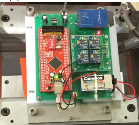
To verify the proposed algorithm a hardware implemented using four MPU9150 IMU sensors made by InvenSense Inc. [23]. These four sensors are located in a way that forms a
planar IMU array as shown in Fig. 2. The LPC1768 ARM microcontroller [24] is selected as the main processor of this multi-IMU board. The I2C protocol is used as the communication method to collect the data of four IMU sensors. As I2C is a 2-wire serial interface, using an optimal firmware in C programming, the time difference between collecting data of each sensor is less than 0.2 ms which compared to the sampling frequency rate is negligible. Moreover, if only measurement from gyroscope or accelerometer is needed, this time will be less than 0.12 ms. In this hardware, General Purpose Input Output (GPIO) of the microcontroller is defined as I2C interface. Two GPIOs are used for SCL and SDA to collect measurement data. In this way, the limitation on the number of IMUs is defined by the number of available GPIOs on the microcontroller. Since in dynamic test the hardware rotates continuously, it is impossible to send data to the host computer via USB connection; therefore, a SD Card module is deployed to store the measured data.
4- Experimental results
Based on the designed experimental setup, three sets of experiments are arranged to collect data in order to verify the real noise reduction capability of multi-IMU sensor configuration. The first set of experiments cover the static test in which the multi- sensory system is subjected to zero input. As for the second and third sets of experiments, the array of sensors are dynamic in two different modes, namely, turning with a fixed angular velocity and oscillating with a period. 4- 1- Static experiment
In this section, the results of a static experiment performed by the hardware are demonstrated. A 2-hour zero rate experiment was conducted with the sampling frequency fs=200Hz for both
gyroscope and accelerometer. The purpose of this test is to combine sensor measurements when IMU array is motionless to obtain ARW and VRW values. First, the mean value of the measured data is subtracted from the entire sample data in order to remove static bias from the measurement values, then, unbiased data of the four sensors are combined and filtered by the information form of steady state Kalman filter. The root Allan variance plot of gyroscopes and accelerometers only for
1
( )
(t)dt
+
Ω
=
k∫
Ω
k
t k
t τ
τ
τ
(36)(37)
(38) 2
2 2
1
1
( )
[
]
2(N 2n)
=( )
( )
+ −
Ω
− Ω
=
−
∑
k nk
k
k n
A
σ
τ
τ
τ
2 2
( )
=
A
τ
ARW
σ
τ
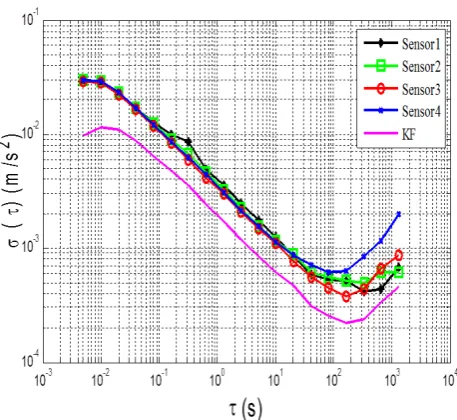
z axis is shown in Fig.3 which indicates that ARW error for
the combined gyroscope signal is around 0.0022 (°/√s ) that
has reduced up to 2.45 times with respect to the single sensor. The results of ARW and VRW coefficients of 2-hour static data is shown in Table 2. In order to investigate the effect of the parameter Q on ARW and VRW reduction, the root Allan variance plot with different values of bandwidth is shown in Fig.5 that indicates by increasing Q and the filter’s bandwidth, reduction of random errors in MEMS inertial sensors is still %50 or two times less compared to one sensor.
The root Allan variance in Fig.6 illustrates the result before and after filtering. As both curves in a shorttime are the same, it is clear there is no reduction in ARW error. In fact, this result proves that for the reduction of stochastic error of an inertial sensor, the only possible solution is to increase the number of sensors. 4- 2- Dynamic experiment
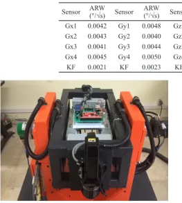
In this study, the dynamic tests for gyroscopes was conducted by a 3-degree of freedom turntable as shown in Fig. 7. The table rotates 360 degrees around z-axis and only 70 degrees around x and y axes; thus, constant rate tests have been performed by z-measurement.
Sensor ARW(°/√s) Sensor (°/√s)ARW Sensor ARW(°/√s) Sensor (m/sVRW2/√s)
Gx1 0.0108 Gy1 0.0107 Gz1 0.0126 Az1 0.0048 Gx2 0.0095 Gy2 0.0094 Gz2 0.0087 Az2 0.0048 Gx3 0.0106 Gy3 0.0111 Gz3 0.0100 Az3 0.0046 Gx4 0.0103 Gy4 0.0103 Gz4 0.0108 Az4 0.0048
Table 1. ARW and VRW coefficients of 24-hours static test
Fig. 3. Root Allan vaiance plot of z-axis of gyroscope Fig. 5. Root Allan variance plot of fused data by different bandwidths
Fig. 6. Root Allan variance plot of a single sensor before and after filtering
The hardware which contains IMU array is attached to the table tightly. The sampling frequency is 200Hz like the static test. The measurement data range for all gyroscopes is set to 2000°/s. The first part of the dynamic test is a constant rate test in which IMU array rotates with six different values
of angular velocities, namely ω=150, 90, 60, 42, 24 and
12°/s, continously. The duration of each test is set to 10 min.
Standard deviation (1σ) is used to evaluate and compare
the results of the fused data with different bandwidths. As
measured, 1σ for all sensors are not identical, for comparison the average of 1σs of all sensors, σm, is used to investigate
improvement of the fused data defined as:
where Ns is the number of sensors.
A comparison is also made by the sensor with the highest
standard deviation. Table 3 summarizes the obtained σm and
1σ of all gyroscopes in z-axis with different rates. Table 4 summerizes the results for ω=150°/s. The results presented
in this table indicate that the performance of the designed filter is degraded by increasing the bandwidth. For the constant rate test, a comparison between Kalman filter, with mimimum/maximum value of bandwidth, and a simple averaging method is made. To see its result refer to Fig. 8.
Computed by averaging method, 1σ of the combined data is 0.2273°/s, when ω=150°/s that is higher than the value
obtained by Kalman filtering even for the large bandwidth. for the practical purposes, the bandwidth of 60Hz is too much. Therefore, it is reasonable to tune the filter by smaller
value of bandwidth the accuracy of the fused data by higher than 2 times compared to the simple averaging method. Table 5 summerizes the results for the constant rate test with 90, 60, 42, 24 and 12 °/s up to 20Hz.
4- 3- Oscillating test
The second dynamic test for IMU array is the oscillating test in which a periodic signal is applied to the turntable, including IMU array. Contrary to the constant rate test which had a low dynamic characteristics, driven by an oscillating input signal, the turntable oscillates in a periodic manner. In this case, the bandwidth of the Kalman filter is an important issue because it should be able to reproduce the signal without amplitude attenuation. Here, a 120-second oscillating test by a periodic signal with the period 4 sec, the amplitude 45°/s, and the sampling frequency 200 Hz is performed. Note that this signal does not have a sinusoidal form, but it has the frequency 0.25 Hz. The same as the constant rate test, measurement range for gyroscopes was set to 2000°/s. In Fig.
Sensor ARW(°/√s) Sensor (°/√s)ARW Sensor ARW(°/√s) Sensor (m/sVRW2/√s)
Gx1 0.0042 Gy1 0.0048 Gz1 0.0054 Az1 0.0041 Gx2 0.0043 Gy2 0.0040 Gz2 0.0040 Az2 0.0038 Gx3 0.0041 Gy3 0.0044 Gz3 0.0041 Az3 0.0035 Gx4 0.0045 Gy4 0.0050 Gz4 0.0047 Az4 0.0037 KF 0.0021 KF 0.0023 KF 0.0022 KF 0.0020
Table 2. ARW and VRW coefficients for 2-hour static test experiment
Fig. 7. 3 degree of freedom turn table was used to analyze the performance of the IMU array in constant and oscillating rate
experiment.
Table 3. Standard deviation for z-axis of gyroscopes with different rates
Table 4. Results of constant rate test for ω=150 °/s with different bandwidths
1
1
=
=
∑
Nsm i
i s
N
σ
σ
(39)Rate
(°/s) Gz1(°/s) (°/s)Gz2 Gz3(°/s) (°/s)Gz4 (°/s)σm
ω=12 0.1152 0.0929 0.0936 0.0924 0.0985
ω= 24 0.1243 0.0884 0.0883 0.0874 0.0971
ω= 42 0.3516 0.1352 0.1160 0.1151 0.1794
ω= 60 0.3745 0.1263 0.1314 0.1391 0.1928
ω= 90 0.5602 0.1587 0.1654 0.7089 0.3476
ω= 150 0.6389 0.1923 0.1850 0.1885 0.3011
BW
(Hz) σKF σm/σKF σgz1/σKF
0.0259 5 0.0983 3
0.1037 10 0.1276 2.3597 5.007 0.2332 15 0.1426 2.2225 4.4803 0.4146 20 0.1524 1.9757 4.1922 0.6479 25 0.1597 1.8854 4 0.9330 30 0.1654 1.8204 3.8627 1.2699 35 0.1701 1.7701 3.7560 1.6586 40 0.1741 1.7294 3.6697 2.5915 50 0.1805 1.6681 3.5396 3.7318 60 0.1852 1.6258 3.4497
2 3
(° )
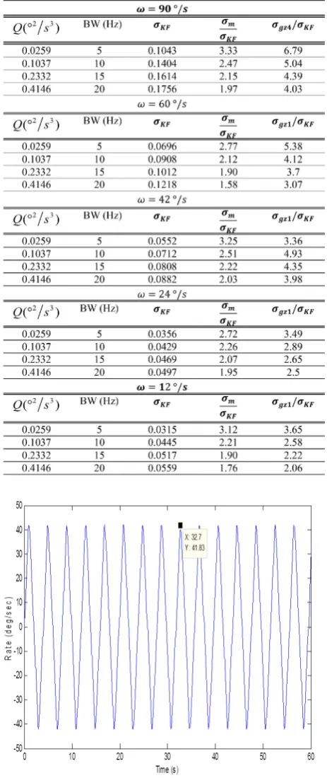
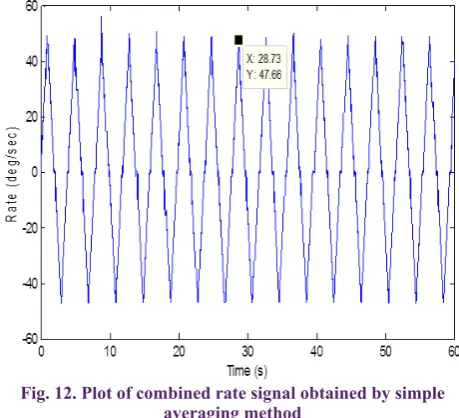
10, a measurement of all sensors during 60 s is shown. As it is clear, the amplitude has increased to 64.53 °/s and most of the measured values are higher than 45°/s. Fig.11 illustrates the
combined rate signal by Kalman filtering with BW=1 Hz
while the maximum amplitude has reached to 41.83°/s. This means that the Kalman filter cannot accurately reproduce the dynamic characteristics of the input rate signal. To obviate this problem, the input rate signal is filtered by Kalman
filter with BW=2Hz which is eight times higher than the
frequency of the input signal. Fig. 12 shows that the fusion
of the measurements with BW=2Hz can reproduce dynamic
characteristics of the input signal. The maximum amplitude is 44.96°/s that is very close to the amplitude of the input signal. In order to show the advantage of the proposed Kalman filter, its results are compared with the averaging method. As illustrated in Fig.12, by applying averaging
method, the 1σ error of the combined rate signal is higher
than Kalman filtering.
5- Conclusion
In this paper an IMU array with four low-cost low-accuracy sensors are implemented to fuse their measurements in order to increase the accuracy of the sensory system compared to one sensor. By lowering the time difference between sensors to 0.2 ms for both gyroscope and accelerometer data, it is feasible to cover a lot of actual input signals. By collecting
Fig. 8. Results of measurement fusion by simple averaging method and Kalman filter with BW=5Hz, 60 Hz
Table 5. Results of constant rate test with the rates ω=90,60,42,24,12°/s
data for 24 hours and using Allan variance method, real information about random errors of the inertial sensors was collected. An information form of steady state Kalman filter was designed to combine data from both gyroscope and accelerometer. In this setup, measured data are combined by a minimum-mean-square error algorithm that reduces the dimension of the data for steady state Kalman filter and decreases the computational complexity. To evaluate the performance of the multi-IMU, a 2-hour static experiment was performed, whose results show that the ARW and VRW errors for z-axis are reduced up to two times compared to the same errors from one sensor. Also, the results of constant and oscillating rate tests, conducted by 3-DOF turntable,
show that the 1σ error decreases by a factor of 3.37 compared to σm. Choosing appropriate bandwidth multi-sensor fusion
algorithm enables us to reproduce dynamic characteristics of input rate signal.
In this paper, the results of multi-sensor fusion problem were addressed with four sensors that may not be an optimal choice for all applications. The optimum number of sensors that reduce the measurement error effectively could be an aspect of the future work for this study. Another important issue that could be addressed in the future is the synchronized data collection of all sensors. In this research, we tried to reduce the time difference between sensors down to 0.2 ms, but it is more reasonable to minimize this time, especially when the number of sensors is increased or with high dynamic input rate signal.
References
[1] D.S. Bayard, S.R. Ploen, High accuracy inertial sensors from inexpensive components, in, Google Patents, 2005.
[2] H. Chang, L. Xue, W. Qin, G. Yuan, W. Yuan, An integrated MEMS gyroscope array with higher accuracy output, Sensors, 8(4) (2008) 2886-2899.
[3] H. Chang, L. Xue, C. Jiang, M. Kraft, W. Yuan, Combining numerous uncorrelated MEMS gyroscopes for accuracy improvement based on an optimal Kalman filter, IEEE Transactions on Instrumentation and Measurement, 61(11) (2012) 3084-3093.
[4] C. Jiang, L. Xue, H. Chang, G. Yuan, W. Yuan, Signal
processing of MEMS gyroscope arrays to improve accuracy using a 1st order markov for rate signal modeling, Sensors, 12(2) (2012) 1720-1737.
[5] L. Xue, L. Wang, T. Xiong, C. Jiang, W. Yuan, Analysis of dynamic performance of a Kalman filter for combining multiple MEMS gyroscopes, micromachines, 5(4) (2014) 1034-1050.
[6] H. Martin, P. Groves, M. Newman, R. Faragher, A new approach to better low-cost MEMS IMU performance using sensor arrays, in, The Institute of Navigation, 2013.
[7] M. Tanenhaus, D. Carhoun, T. Geis, E. Wan, A. Holland, Miniature IMU/INS with optimally fused low drift MEMS gyro and accelerometers for applications in GPS-denied environments, in: Position Location and Navigation Symposium (PLANS), 2012 IEEE/ION, IEEE, 2012, pp. 259-264.
[8] I. Skog, J.-O. Nilsson, P. Handel, An open-source multi inertial measurement unit (MIMU) platform, in: Inertial Sensors and Systems (ISISS), 2014 International Symposium on, IEEE, 2014, pp. 1-4.
[9] R. Rasoulzadeh, A.M. Shahri, Implementation of A low-cost multi-IMU hardware by using a homogenous multi-sensor fusion, in: Control, Instrumentation, and Automation (ICCIA), 2016 4th International Conference on, IEEE, 2016, pp. 451-456.
[10] G. Yuan, W. Yuan, L. Xue, J. Xie, H. Chang, Dynamic performance comparison of two Kalman filters for rate signal direct modeling and differencing modeling for combining a MEMS gyroscope array to improve accuracy, Sensors, 15(11) (2015) 27590-27610.
[11] I. Skog, J.-O. Nilsson, P. Händel, A. Nehorai, Inertial Sensor Arrays, Maximum Likelihood, and Cramér–Rao Bound, IEEE Transactions on Signal Processing, 64(16) (2016) 4218-4227.
[12] A. Unknown, IEEE Standard Specification Format Guide and Test Procedure for Coriolis Vibratory Gyros, IEEE Standards, 1431 1-79.
[13] N. El-Sheimy, H. Hou, X. Niu, Analysis and modeling of inertial sensors using Allan variance, IEEE Transactions on
Fig. 11. Plot of combined rate signal obtained by Kalman filter
instrumentation and measurement, 57(1) (2008) 140-149.
[14] R.J. Vaccaro, A.S. Zaki, Statistical modeling of rate gyros, IEEE Transactions on Instrumentation and Measurement, 61(3) (2012) 673-684.
[15] R.E. Kalman, R.S. Bucy, New results in linear filtering and prediction theory, Journal of basic engineering, 83(1) (1961) 95-108.
[16] D. Simon, Optimal state estimation: Kalman, H infinity, and nonlinear approaches, John Wiley & Sons, 2006.
[17] R.S. Bucy, P.D. Joseph, Filtering for stochastic processes with applications to guidance, American Mathematical Soc., 1987.
[18] M. Grewal, A. Andrews, Kalman theory, theory and practice using MATLAB, in, John Wiley & Sons, Inc, 2008.
[19] C. Chen, Linear System Theory and Design. New York: Holt, Rinehart and Winston, Decoupling with stability for linear periodic systems, 765 (1984).
[20] Q. Gan, C.J. Harris, Comparison of two measurement fusion methods for Kalman-filter-based multisensor data fusion, IEEE Transactions on Aerospace and Electronic systems, 37(1) (2001) 273-279.
[21] N. Assimakis, M. Adam, A. Douladiris, Information filter and kalman filter comparison: Selection of the faster filter, International Journal of Information Engineering, 2(1) (2012) 1-5.
[22] D.W. Allan, Statistics of atomic frequency standards, Proceedings of the IEEE, 54(2) (1966) 221-230.
[23] InvenSens MPU9150 Motion Sensor Document number: PS-MPU9150A, Rev4.0
[24] NXP (Phillips),LPC17xx 32-bit ARM Cortex-M3 microcontroller, Rev. 5.3.
Please cite this article using:
A. M. Shahri and R. Rasoulzadeh, Implementation of a Low- Cost Multi- IMU by Using Information Form of a Steady State Kalman Filter, AUT J. Elec. Eng., 49(2)(2017)195-204.