Consumption-Based Asset Pricing with Recursive Utility

Iranian Journal of Economic Studies

Journal homepage: ijes.shirazu.ac.ir

Consumption-Based Asset Pricing with Recursive Utility

Marjan Radniaa, Mosayeb Pahlavanib, Mohammad Nabi Shahiki Tashc, Reza Roshand a. Department of Economics, University of Sistan and Baluchestan, Zahedan, Iran.

b. Department of Economics, University of Sistan and Baluchestan, Zahedan, Iran. c. Department of Economics, University of Sistan and Baluchestan, Zahedan, Iran. d. Department of Economics, Persian Gulf University, Bushehr, Iran.

Article History Abstract

Received date: 5 September 2017 Revised date: 7 October 2017 Accepted date: 14 October 2017 Available online: 1 November 2017

In this paper it has been attempted to investigate the capability of the consumption-based capital asset pricing model (CCAPM), using the general method of moment (GMM), with regard to the Epstien-zin recursive preferences model for Iran's capital market. Generally speaking, recursive utility permits disentangling of the two psychologically separate concepts of risk aversion and elasticity of intertemporal substitution which are constrained to be equal to the inverse of each other for the traditional time-additive utility functions. Rather than using the stock market as a proxy for wealth, we constructed a more comprehensive return which is the weighted average of stock index return, labor wage growth (as a proxy for human capital return), housing return and deposit return. The empirical results demonstrate that the signs of the coefficient of the relative risk aversion and the intertemporal elasticity of substitution are the same, which means that investors have homogeneous attitudes toward the risk across the states of nature and the risk over time in Iran but different ones in their values. Therefore, the assumption that the relative risk aversion is equal to the reciprocal of the elasticity of substitution is not valid in Iran's stock market.

JEL Classification: G10

G11 G12 C52 G02 E43

Keywords: Asset-pricing theory Behavioral parameters General method of moment Recursive utility

1. Introduction

Investigating the relationship between the risk and the return, as the two main pillars of the investment decision, is of particular importance in financial literature. Several models have been proposed by economists, among which the standard capital asset pricing model (CAPM), presented by William Sharp (1964), has been more acceptable, because of the definition of a simple mathematical linear relation between the risk and the return in the financial industry. (Pamane and Vikpossi, 2010). In this model, investors are assumed to maximize their preferences for consumption and the preferences are represented

 [email protected]

by expected utility theory (EUT). (Dong He and Guo, 2017)

This model measures the risk of the bounds through its yield covariance with the stock market return.

Moreover, consumption based asset pricing model (CCAPM) of Lucas and Breeden (1978), offers a popular framework in relation to the valuation of assets with the consumption-investment decision, considering the exchange economy with homogeneous preferences and asset prices are determined by the process of selecting an asset portfolio, assuming that the agents consume all their wealth only after a period of time. This fact disregards the complexity of inter-period consumption decisions and the interaction between the consumption and asset portfolio selection.

Also, the asset risk is determined by the covariance of the asset’s return with marginal utility of consumption and consumer preferences in this model have been presented with a constant relative risk aversion power utility function. (Wang and Yang, 2016)

This model utilizes the standard separation power function and the completely limiting assumptions, such as the inverse of the risk aversion coefficient, the elasticity of the intertemporal substitution (EIS), and the impossibility of separating them from each other, to explain the relationship between the returns and the consumption. The relative risk aversion describes the consumer’s willingness to stabilize the consumption in the natural states and therefore a risk-attitude approach is considered, but the intertemporal substitution describes the tendency toward smoothing the consumption over the time and therefore it is an attitude toward the time risk.

This model can only be adapted to the observed levels of consumption growth and asset returns, which is an unjustifiably large coefficient of relative risk aversion (investor risk) of the investor. Also, the high returns and on the low risk-free rate of assets create the risk premium or excessive expectation returns. In other words, the stock returns are so large that they are impossible to be explained by the changes in the actual consumption growth rate. (Mehra, 2006)

Therefore, the inability of the power utility function to explain the behavior of the observations has led to the investigation of various methods and forms of other utility functions. In this regard, the use of recursive utility functions, presented by Epstein and Zin (1991), has been of great interest (Guo and Dong He, 2017).

Recursive utility provides the important generalizations of the standard utility model, used in asset pricing models, among which, its more flexibility compare to the risk and the intertemporal substitution, is the most prominent. Also, unlike the utility function, in which the CRRA and the EIS reciprocity are inverse and cannot be separated, the risk aversion factor is not necessarily equal to intertemporal substitution, under the recursive preferences.

and the empirical facts (Suzuki, 2016). Therefore, in this study, it has been attempted to make adjustments to explain the return and risk concepts and the pricing of assets for Iran's capital market. For this purpose, the behavioral parameters for the annual stock market data of Iran during 1988-2014, will be estimated by introducing a class of Epstein-Zin (EZ) recursive preferences that allows for the separation of relative risk the aversion coefficients and the intertemporal substitution and using the GMM method.

In general, the contribution of this research for Iran's capital market can be described as follows:

Using EZ recursive utility function instead of the power utility function in optimizing the behavior of economic agents.

Using a comprehensive and homogenous combination of market returns, housing returns, labor wage, and deposit return as a wealth Portfolio

- Estimating the proposed recursive utility function through the GMM. This paper has been organized as follows: the theoretical foundations are presented in section 2, which includes a review of the CCAPM with the recursive utility and GMM method. In section 3, the data will be described and the empirical results will be discussed. Finally, in Section 4, the experimental results of the economic model and conclusion are presented.

2. Modeling and Testing Background

2.1 An asset pricing model based on consumption (CCAPM)

The basis of the CCAPM is that the asset prices are derived from the macroeconomic risks and they are directly related to the consumption (inter-temporal consumption rate). In this model, it is assumed that all the investors have a long horizon of time and they are homogeneous in terms of the preferences. This assumption helps the researchers to generally evaluate the economy by studying the behavior of the representative agent.

In this model (CCAPM), Lucas (1978), provides a complete theoretical test of the behavior of the equilibrium asset price of a pure exchange economy and the yield covariance here, known as the beta consumption (βc), is considered as a systematic risk measure with the cumulative growth of the consumption. In other words, it can be stated that the (βc) is a standard to measure the systematic tendency of the stocks to follow the movements of the market (Mohammadzade et al., 2015).

The CCAPM model is more widely used than the CAPM model, and as the beta consumption combines the nature of interruptible portfolio decisions and simultaneously considers other forms of wealth beyond the stock market, it is the basis for understanding the relationship between wealth, consumption and the risk aversion of the investors.

To explain this model, it is assumed that in a single commodity economy, the consumer tries to maximize the current value of its expected utility lifetime:

0

max t j ( t j)

j E U C



 

 

 







Where

C

_{t j} is the consumption of the investor in the period

t



j

,

U C

(

t j

)

is a

strictly concave utility function, Et is the expectation operator conditioned on time t information and 0



1 is the subjective discount factor, which depends on the subjective rate of the investor preferences. When this parameter is large, the agent puts more weight on the future and less weight on the present. It is also assumed that the consumer has a time-separable utility function with the constant risk aversion coefficient as follows:

1 ( ) 1 t t C U C    

 ,



0 (2)

Where



represents the relative risk aversion coefficient and the curvature of the utility function. The CRRA utility function exhibits the decreasing absolute risk aversion, which means that when the initial wealth increases, aversion towards the risk diminishes. The CRRA utility function exhibits constant relative risk aversion, therefore the proportion of the wealth, that agents want to expose to risk, remains unchanged with the wealth. (Campbell, 1999).

The Euler equation which describes the optimal consumption in j 1 is shown in the equation 3:

(3)

where

1



R

_{i t,1} is the return on the asset i. Relation 3 indicates that in the

equilibrium conditions, the marginal utility which is lost from the foregoing current consumption is equal to the discounted expected utility to be gained from investing in the asset i. By re-arranging (3), the asset pricing model is obtained:

1

, 1

( )

(1 ) 1

( )

t

t i t

t U C E R U C          _    (4)

If the investor is highly risk averse, the present value of future payoffs will also be low. Thus, the basic pricing equation under the power utility with

differentiating (2) and substituting into (4) becomes:

(5)

Also, under this utility function, the stochastic discount factor or the pricing kernel is: 1 1 1 ( ) ( ) t t t t t

U C C

M

U C C

           _{  }

 _{ } (6)

1 , 1

( _t) _t ( _t )(1 _{i t} )

U C 



E U C_  _ R _ _

1

, 1

1 t (1 )

t i t

2.2 The asset pricing model modification based on the recursive utility The standard time-separable power utility C-CAPM fails to explain the relationship between the risk and the returns due to the multiple constraints, including the reverse and reciprocal relationship between the risk aversion coefficient and the elasticity of the intertemporal substitution. Consequently, several adjustments have been made to the function of preferences by the economists. One of the most important adjustments has been presented by EZ (1991). By presenting a class of preferences, they let the relative risk aversion coefficient and time preference to be independent of each other. Therefore, the risk aversion coefficient in their model does not imply the tendency to smooth the consumption over the time.

In this type of preferences, the utility function is presented as follows: (Hyde and Sherif, 2005)

(7)

In this recursive preference set up, E_t is the conditional expectation operator at time t, C_t is consumption at the beginning of period t,  1 is the subjective discount factor (1 (1) given  0), 1

(1 )

_{ }  _and (1 )(1 1 )

     . The coefficient of relative risk aversion (RRA) is equal to



(

0



) while the elasticity of intertemporal substitution (EIS) is  _{ (1} ₎1_.

In this framework, the asset is priced by its covariance with both the consumption growth rate and the return on a wealth portfolio. Thus, the features of the consumption-based pricing model will also be included in this model.

In the Epstein-Zin model, the wealth of agents is formulated as:

1 ( )(1 , 1)

t t t w t

W _  W C R _ (8) In which the returns are invested in all the wealth. Since the total wealth involves the consumption of the future periods, which are virtually invisible, Epstein-Zin applied the proxies of the return on the stock market in their model.

Given the budget constraint of the wealth, the problem of maximizing the intertemporal utility of the agent is as follows:

Under recursive preference, the representative consumer-investor’s problem is as follows:

1 1

(1 ) 1

1 1

maxU C E Ut( t, t t ) (1 )Ct E Ut( t )

 

  

   

 _      _ (9)

Subject to:

1 1, , , 1 1,

2

, ( )

N

t t t j t j t t j

t W_ I R  R _ R



 

  _   _







(10)

1 1

(1 ) 1

1

(1 ) ( )

t t t t

U C E U

 

  











 _{ } 

They elaborate the weight of the

i

thasset in the wealth portfolio as:

, ,

(

) /

i t

Q P Z

i t i t

I

t





Where

, 1

( ) N

t i t i t i

I Q P z







and

, 1 1 N j t i  





(11)

The stochastic discount factor, obtained from the maximization problem is:

1 1

1

1 , 1

, 1

1

(1 )

1

t

t i t

t w t

C M R C R  _            _{ }       _{ } _          (12)

Therefore, Euler's equation for the EZ model will be:

1 1 1 , 1 , 1 1

1 (1 )

1 t

t i t

t w t

C E R C R  _        _{     }  _{ }      _{ } _       _{ }      (13)

Based on this equation, it will be demonstrated that the marginal rate of the substitution of the EZ utility function depends on the overall consumption return and the return on wealth, while the marginal rate of the substitution of CRRA depends only on the consumption growth (Wang et al., 2016).

In order to maintain and identify the parameter 1

(1 )

 _{ }  _{, it is} necessary to consider the following equation which correlates market returns with consumption growth:





1

1

, 1

1 1 0

t

t w t

t C E R C        _{   } _ _{      } _  _{   }  _  _   (14)

The Euler equation derived from the EZ recursive utility, consists of three behavioral parameters namely the subjective discount factor, the coefficient of the relative risk aversion and the intertemporal elasticity of the substitution. This utility function allows the separation of the two behavioral concepts: the coefficient of the relative risk aversion and the intertemporal elasticity of the substitution which are considered inverse based on the power utility function.

Regarding the invisibility of the wealth variable, EZ, used the stock market return as a substitute, instead of the return on wealth, in order to calculate it in the asset pricing model. Since this variable does not include an important part of the asset forms, namely the human capital and housing, in this research, we follow Campbell study (1996) of the average weighted return on the stock index, the labor wage return (as a proxy for human capital), the housing return and the long run private sector deposit return have been applied as a proxy for the wealth return.

2.3 Estimation of Euler Equation Parameters Using GMM

The mentioned method has many great advantages. first, this technique can be used to estimate the parameters of the model without any assumption about the distribution of the variables; second, in this method, the occurrence of the correlation between the variables and white noise components will be prevented due to the use of the instrumental variables, and ultimately, the GMM method allows the serial auto-correlation to exist among the disruptive components.

In general, the purpose of the GMM method is to produce a family of appropriate moment conditions in order to create a square criterion function which could be minimized by the estimators.

The criterion function is constructed in a way that the GMM estimators will be asymptotically normal and have an asymptotic covariance matrix which can be estimated compatibly.

To estimate the Equation (13) by using the GMM method, first, it is necessary to define the moment conditions appropriately. So, initially, we assume that there is a sample of the n-

dimensional



X

t

:

t



1,...,

T



time series observations (Smith, 1999).

The constraints that the hypothesis

H

₀ applies to data moments can be

elaborated as follows:



1



1 1

( , , ) 0

( , , ) ( , ) ,

t t

t t t t

E g X Z

g X Z U X Z



 



 



  (15)

where, E is an unconditional expectation operator, the elements of the k -vector



are unobservable that must be estimated,

X

_t1is a l1vector of

variables, U X( _t₁, ) is a function of d and

Z

tis a r1 vector of visible instrumental variables at t time point.

.The dr-vector of conditions vector g X( _t₁,Z_t, ) is obtained by

multiplying the vector,

U X

(

_t1

, )



by each element in the vector

Z

_t.

The Euler equation (14), for the ith component of

U X

(

_t1

, )



is:

1 1

1

1 , 1

, 1

1

( , ) (1 )

1 t

i t i t

t w t

C

U X R

C R  _                     _{ } _         

, (16)

Where 1

1 1, 1 , 1

, 1

1

, , ,..., 1

t

t t N t

t w t

C

X R R

C R         _ _   

,



( , , )

  

, t 1

t

C C

 _{is a}

measure of the growth

in real consumption,

R

_{w t,}₁ is the aggregate wealth return and consist of

Since Equation (13) impliesE U X_t



( _t1, )



0, so it follows by iterative expectations from



(

t 1

, )

t





(

t 1

,

t

, )



0

E U X

_





Z



E g X

_

Z





(17)

where



is a vector of m parameters governing the distribution of X and

(.)

g is a vector of q functional forms. The GMM estimator replaces



( t 1, t, )



E g X _ Z  with its sample analogue and when the size of the sample widens, in



₀ value goes to zero.

In other words,



must be selected in such a way that the sample moments are close to the moment of the statistical population.

The GMM estimator will minimize the amount of

Q

_T

( )



so that

( ) ( ) ( )

T T T T

Q  g  W g  (18)

In the above statement,

W

_T is a

dr dr



semi-definite symmetric

weighted matrix positive, defined as:

1

T T

W V  (19)

This matrix will minimize the variance for estimating



among GMM estimators and

V

_T estimates the compatibility of the symmetric covariance

matrix of 12 _{( )}

T

T g



.

Hansen (1982) also shows that



_T is a consistent estimator of



₀and has a

normal asymptotic distribution with covariance matrix, (G V G₀ 1 ₀)1 that

0

( ) T

g

G E 





 

 _{ } _ and

V



E g



t

( ),



g

t

( )







.

In many cases, the moment conditions are greater than the unknown parameters (dr> k) and the system is over-identified. In other words, the number of dr-k linear combination remains, which will not be considered in the estimation.

If the model is correctly specified, the remaining dr-k can go to zero. Therefore, the null hypothesis is tested by determining if the over-defined limitations remaining are to be (near) zero.

Hansen (1982) presented the J test for over-defined limitations to measure how close the zero sample moment conditions are:

2

(

)

asy

T T T dr k

J



T Q





 (20)

instrumental variables are properly selected and the model is properly fitted. If the value of this statistic is smaller than the statistics of the distribution table of

2



, the H₀ hypothesis, about the appropriateness of the instruments, will be verified.

3. Empirical results 3.1 Data

In order to estimate the model and create wealth portfolio, the data have been extracted from the Central Bank of Iran and the Tehran Stock Exchange. The desired data is in annual period, 1988 and 2015. The main variables used in this study, which are calculated on the basis of the 2011 price index with real values, are:

- Stock return, constructed from Tehran stock market index which has been calculated, using the following equation (P is the stock price index), 1

1

t t t

p p

p





 _.

- Housing return for private domestic units constructed from investments in urban areas and estimated cost of one meter square by the private sector for completed buildings;

- Growth rate of private sector consumption expenditure;

- Wage growth which is extracted from data on the minimum wage of the workforce;

- Short risk-free rates the amount of deposits held by the private sector department.

Also, in this study, we followed Campbell (1996) to measure a comprehensive portfolio of wealth, including a balanced combination of stock index return, labor wage growth, housing return and deposit return.

It is worth noting that, there is an appropriate weight for each asset for calculation of the returns of the mentioned portfolio, and in fact the produced portfolio includes the return of the types of assets in which the return on each asset is weighed by an appropriate factor.

It should be noted that the weights of each asset are as follows:

- The "value of market transactions" has been used for the returns of the total stock index,

- The "private sector investment in the housing sector" has been used to calculate the weight of housing stock returns.

Also, data on labor income and the volume of private sector deposits are considered as the weight of return in income and deposit return respectively (Roshan et al., 2013)

The form of creating the portfolio used in the research is described in general term: (Iyiola et al., 2012; and Roshan et al., 2013)

∑ ∑

∑

where R: The vector of return of each asset in agent portfolio consists of (stock: return of total index of stock market; deposit: return of long term deposits; housing: return of changes of housing price). vi: The volume of each asset in household’s portfolio; V: total volume of assets that have been used in household’s portfolio; Wi: weight of each asset

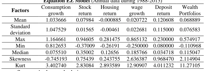
Table 1 provides statistical characteristics of variables used in model:

Table 1. Statistical Characteristics of Variables Used in Estimating Euler

Equation EZ Model (Annual data during 1988-2015)

Factors Consumption

growth

Stock return

Housing return

wage growth

Deposit return

Wealth Portfolios Mean 1.033666 0.07984 -0.000885 0.020722 0.120608 0.068889 Standard

deviation 1.047529 0.01565 -0.00461 0.022681 0.115000 0.076583 Max 1.164661 0.94605 0.281475 0.865132 0.230000 0.574917 Min 0.812653 -0.37009 -0.26191 -0.250000 0.080000 -0.110968 Median 0.075510 0.35002 0.12656 0.185766 0.034718 0.115047 Skewness -0.745193 0.75439 0.243755 2.636387 0.968470 2.114904 Kurt 3.402740 2.83084 2.893589 12.90907 4.011232 11.27105

Source: Authors calculation

3.2 Stationarity test

Despite the fact that the GMM method does not require a lot of assumptions about the variables, it is important to examine the stationarity of the variables. Therefore, before performing any estimation, we have used the Augmented Dickey-Fuller test is conducted to determine the stationarity of time series data applied in this paper.

For the time series



y t_t, 1, 2,...



, we have made a first-order

auto-regression or AR(1) process with constant: y_t   y_t1_t, where



_t is the

white noise time series. If  1, there is no unit root,

y

_tis stationary. If

1

  , there is a unit root in time series, which means that

y

_tis non-stationary. A convenient reformulation is:

 

y

_t



y

_t₁





_t, where

 

 1.

Therefore, using the unit root test, the H₀: 0 hypothesis was tested (Xu-song et al., 2006)

Based on the empirical result, we conclude that all of time series are stationary.

3.3 Estimations of the parameters

consider two points. First, selecting more instrumental variables does not necessarily lead to the improvement of the model. Second, these variables should be selected based on their application in making the estimation more accurate and understanding the parameters.

In this research, the selected instrumental variables for the model justified by the recursive utility function, are as follows:

c, house(-2), deposit(-1) ,labor(-2), house(-3) with Initial values 1.6 ,2.1 and 4.6 for

  

, , .

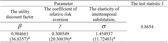
Table 2. Estimation of the parameters of the Euler equations in EZ model with GMM

Parameter The test statistic J The utility

discount factor

The coefficient of relative risk

aversion

The elasticity of intertemporal

substitution,

8.8654







0.984661 (36.8357)*

0.300549 (20.30839)*

1.454937 (11.72483)* Source: Authors calculation

The estimation results have been demonstrated in Table 2. The values of the parentheses are related to the t test and indicate the significance of the estimated parameters at the 95% confidence level.

The GMM estimator compatibility depends on the validity of non-serial autocorrelation assumption between error terms and instruments that can be examined by the J test first presented by Hansen. The statistic of table J is equal to



2_1,5



3 / 841

and the values of the model are smaller than this number, so

the null hypothesis and goodness of the choice of instruments in the model is confirmed.

Also, considering the obtained values for the behavioral parameters of the model, we observe that the discount factor



is significant at 5% level, and since this number is very close to 1, it can be concluded that the consumers are very patient and prefer the future consumption over that of the present. Estimation parameter



in this model is 0.300549, positive sign of this parameter indicate that economic factors are very risk averse. Since the risk aversion coefficient describes the tendency toward the consumption stabilization in the different situations, it can be concluded that the investors in Iran, are risk averse toward the state risk.

parameters cannot be verified.

4. Conclusion and Recommendation

In this paper, GMM method has been used to estimate and test the ability of the Epstein and Zin's (1991) recursive utility models to explain the stock market returns in Iran.

Using consumption growth data and weighted average of stock index return, labor wage growth, private sector deposits return and housing return, we found that there was some evidence supporting the classic CCAPM based on recursive utility and the estimation results accept the Hansen’s J-test, which expresses that the model are correspondent with the data and our model is capable of explaining the stock returns in Iranian financial market.

More importantly, the findings of the present study demonstrate that, the amount of the estimated parameters for the duration of this study is consistent with the theoretical considerations, by adjusting the asset pricing model with the recursive utility function and the relative risk aversion and the intertemporal elasticity of the substitution are quite distinct. Also, their signs are the same, which means that, the investors have a similar-and not equal-attitude toward the state and the time risk in Iran's financial market.

Considering the significance of the results of the estimates, it seems that Epstein-Zin (1991) recursive utility function and the separation of the relative risk aversion coefficient from the elasticity of the intertemporal substitution, is more compatible with the experimental facts in asset pricing issues, rather than the power utility function. Therefore, considering the importance of the relationship between the risk and the return, it seems crucial to conduct more research on the capital asset pricing models.

References

Acharya, V., & Pedersen, L. (2005). Asset pricing with liquidity risk, Journal of Financial Economics, 77, 375–410.

Asprem, M. (1989). Stock prices, asset portfolios and macroeconomic variables in 10 European countries, Journal of Banking and Finance, 13, 589 -612. Bansal, R., & Yaron, A. (2004). Risks for the long run: a potential resolution of

asset pricing puzzles, Journal of Finance, 59(4), 1481-1509.

Breeden, D. T. (1979). An inter-temporal asset pricing model with stochastic consumption and investment opportunities, Journal of Financial Economics, 7, 265-296 .

Campbell, J. Y. (1993). Inter temporal asset pricing without consumption data, American Economic Review, 83,487-512.

Campbell, J. Y. (1996). Consumption and the stock market: interpreting international experience, Swedish Economic Policy Review, 3, 251-299. Campbell, J.Y., & Cochrane, J. H. (1999). By force of habit: a

consumption-based explanation of aggregate stock market behavior, Journal of Political Economy, 107(2), 205-251.

Chen, M. H. (2003). Risk and return: CAPM and CCAPM, Journal of Economic and Finance, 43,369-393.

Darrat, F, A., Li, B. & Park, C. J. (2011). Consumption-based CAPM models: international evidence, Journal of Banking & Finance, 35, 2148-2157.

Epstein, L. G., & Zin, S. E. (1991). Substitution, risk aversion and the temporal behavior of consumption and asset returns: a theoretical framework.

Econometrica, 57(4), 937-969.

Fama, E. F., & French, K. R. (1995). Size and book-to-market factors in earnings and returns, Journal of Finance, 150, 153-154.

Galagedra, D. (2006). A review of capital asset pricing models, Journal of Banking, 43, 1-15 .

Gregoriou, A., & Ioannidis C. H. (2006). Generalized method of moments and value tests of the consumption capital asset pricing model under transactions, Empirical Economics, 32,19-39.

Guo, J., & Dong, X. (2017), Equilibrium asset pricing with Epstein-Zin and loss-averse investors, Journal of EconomicDynamics & Control, 76, 86– 108.

Hamori, S. (1992). Test of CCAPM for Japan: 1980–1988, Economics Letters, 38, 67-72.

Hansen, L., & Singleton, K. J. (1982). Generalized instrumental variables estimation of nonlinear rational expectations models. Econometrica, 50, 1269-1286 .

Hyde, S., & Sherif, M. (2005). Consumption asset pricing models: evidence from UK. The Manchester School, 73, 343-363.

Iyiola, O., Munirat, Y., & Nwufo C. (2012), The modern portfolio theory as an investment decision tool, Journal of Accounting and Taxation, 4(2),19-28.

Kwan, Y. K., Leung, C. K. Y., & Dong, J. (2015). Comparing consumption-based asset pricing models: the case of an Asian city, Journal of Housing Economics, 28, 18-41.

Lucas, R, E. (1978). Asset prices in an exchange economy, Econometrica, 46, 1429-1445.

Mankiw, N. G., & Shapiro, M. D. (1986). Risk and return: consumption beta versus market Beta. Review of Economics and Statistics, 68, 452-459 . Márquez, E., Nieto, B., & Rubio, G. (2014). Stock returns with consumption and

illiquidity risks, International Review of Economics and Finance 29, 57– 74.

Mehra, R., & Prescott, E. C. (1985). The equity premium: a puzzle, Journal of Monetary Economics, 15,145-161.

Mehra, R. (2006). The equity premium puzzle: a review, Foundations and Trends in Finance, 2(1), 1–81.

Mehra, R., & Prescott, E. C. (2008). The equity premium: a puzzle in retrospect. Forthcoming in the Handbook of the Economics of Finance, Edited by G.M. Constantinides, M. Harris and R. Stulz, North Holland.

Mohammadzadeh, A., Shahiki-Tash, M. N., & Roshan, R. (2016), Investigating and comparing some consumption-based asset pricing models: the case of Iran, International Journal of Economics and Financial Issues, 6(4), 1884-1894.

Pamane, K., & Vikpossi, A. E. (2014). An analysis of the relationship between risk and expected return in the BRVM stock exchange: test of the CAPM.

Research in World Economy, 5(1), 13-25

Roshan, R., Pahlavani, M., & Shahiki-Tash. (2013). Investigation on habit formation, risk aversion and inter-temporal substitution in consumption of Iranian households by GMM approach, International Economic Studies,

42(1), 47-56

Smith, D. C. (1999). Finite sample properties of tests of the Epstein–Zin asset pricing model, Journal of Econometrics ,93(1), 113–148.

Sharpe, W. F. (1964). Capital asset prices: a theory of market equilibrium under conditions of risk, The Journal of Finance, 19, 425-442.

Suzuki, M. (2016). A representative agent asset pricing model with heterogeneous beliefs and recursive utility, International Review of Economics & Finance, 45, 298–315.

Wang, C., Wang, N., & Yang J. (2016). Optimal consumption and savings with stochastic income and recursive utility, Journal of Economic Theory, 165, 292–331.

Xiao, Y., Faff, R., & Philip, M. (2013). Pricing innovations in consumption growth: a re-evaluation of the recursive utility model, Journal of Banking & Finance, 37, 4465–4475.