Hybridization of Particle Swarm Optimization with Unsupervised
Clustering Algorithms for Image Segmentation
Wenping Liu, Ethan McGrath, Chih-Cheng Hung, and Bor-Chen Kuo
Abstract
1Unsupervised fuzzy clustering algorithms are one of many approaches used in image segmentation. The Fuzzy C-means algorithm (FCM) and the Possibilistic C-means algorithm (PCA) have been widely used. There is also the generalized possibilistic algorithm (GPCA). GPCA was proposed recently and is a general form of the previous algorithms. These clustering algorithms can be trapped to the local optimal solutions. Hence, optimization techniques are often used in conjunction with algorithms to improve the performance. Some of optimization techniques have been inspired by nature such as swarm behavior. Particle Swarm Optimization (PSO) is one such technique. In this paper, PSO heuristics were combined with FCM, PCA, and GPCA algorithms to improve the overall clustering accuracy of these algorithms. To test the improvement with the PSO, these algorithms were tested on images. The overall effect of adding unique PSO methods was a higher percentage of satisfactory image segmentations.
Keywords: Fuzzy C-means Algorithm, Possibilistic Clustering Algorithms, Particle Swarm Optimization.
1. Introduction
One form of manipulation to derive meaning from an image is segmentation. Segmentation involves dividing an image into distinct regions based on certain similar features to give each region a level of homogeneity. For example, the segmenting of a scanned document into the background and the text components would be a simple segmentation. There are many methods that have been proposed for segmentation. In this paper the concentration will be on segmentation via clustering using objective function optimization techniques.
Image segmentation via clustering is a pattern recognition technique where similar pixels are grouped together in a cluster. Features of the pixels such as
Corresponding Author: Wenping Liu is with the computer science and information engineering at Beijing Forestry University, Beijing, China.
Manuscriptaccepted 18 Aug. 2008.
proximity to other pixels and color can be used as tests to determine if a pixel is similar enough to be added to a set of other pixels. Once similar pixels are clustered together, the image can be segmented into distinct sections where each cluster represents one segment. The pixels in one cluster should be distinct from pixels in another cluster. However, accomplishing this task is currently a challenging problem and much research is being undertaken to improve on the current methods.
Among the techniques used in this paper to segment images are the Fuzzy C-means algorithm, the Possibilistic Clustering algorithm, and the Generalized Possibilistic Clustering algorithm. These algorithms share a common thread in that they utilize a fuzzy clustering scheme. These algorithms sometimes do not find optimal results because they are sensitive to the choice of initial pixel memberships. Therefore, there is room to improve the results of these algorithms, and thus a particle swarm optimization was incorporated to accomplish that task. Using a PSO with image segmentations is not new; however, the methods and heuristics used are unique.
Two methods are utilized to incorporate the PSO. The first method is to run the PSO after the chosen clustering algorithm completes. This method has the benefit of being able to easily measure the improvement since the before and after segmentations of the image are available. The second method is to run a hybrid algorithm that incorporates the PSO into the existing clustering algorithm. This method is harder to measure for the improvement versus running the fuzzy clustering algorithm alone. Since the PSO is intermixed with the fuzzy clustering algorithm, there is only a single segmentation result. Thus, to compare the results of this method, the total number of good segmentations found per image is measured against the amount found by the first method.
These algorithms, because of their fuzzy nature, assign a certain percentage of membership of a pixel to each cluster (it can be zero percent membership). The final results are based on the highest percentage membership of a pixel to a cluster. By only using the RGB values in the clustering, the complexity and number of variables remain low, thus making the tuning of the algorithms less complicated while also producing experimental results that are more straightforward to interpret. Likewise, the images chosen can be
satisfactorily segmented using only color information. The PSO requires heuristics to be chosen which will optimize segmentation. Through experimentation it was found that maximizing the sum of the total pixels in a cluster divided by the mean distance of the pixels to the cluster center seems to produce a good outcome. This new heuristic was invented for these image segmentations. In using this heuristic, the PSO attempts to produce clusters that have many pixels in them but also are compact in terms of having a small color distance between the pixels and the centroid. While the algorithms themselves will often generate a favorable segmentation, the PSO has shown to fix unfavorable segmentations while leaving intact already good segmentations.
The rest of paper is organized as follows. Section 2 covers the FCM, PCA and GPCA algorithms and their origins. Section 3 describes in more detail the integration of PSO with the FCM, PCA, and GPCA algorithms. Section 4 presents the validity and accuracy measures used to judge the segmentation and the experimental results generated using the algorithms. Section 5 presents the conclusions of this research.
2. Previous Work
2.1 Unsupervised Clustering Algorithms
In fuzzy set logic, an element can have a partial or degree of membership to a set. This is in contrast to classical set theory where each element of a set is either a member of the set or not in the set. Therefore, fuzzy clustering differs from crisp or hard clustering in that an element does not need to exclusively belong to a cluster for each iteration of the algorithm. However, there is no rule to prevent an element from exclusively belonging to a single cluster and thus, fuzzy clustering is considered a generalization of hard clustering. To achieve a final segmented result via fuzzy clustering (defuzzification), the elements are divided into hard clusters based on their majority membership to a single cluster at the completion of the iteration of the algorithm.
These unsupervised algorithms operate on a set of data by attempting to minimize an objective or cost function. Some a priori knowledge can be given as initial parameters. In the case of image segmentation, the number of clusters is all that needs to be provided.
2.1.1 The Fuzzy C-means Algorithm
The fuzzy c-means algorithm works by iteratively minimizing an objective function. The objective function is the sum of squares distance between each pixel and the cluster centers and is weighted by membership.
This development of this algorithm is credited to Bezdek [1].
The FCM objective function:
2 1 1 i N j c i j m ij x v J
∑ ∑
u
= = − = (1)where uij represents the membership of pixel xj to the ith
cluster and vi is the centroid of the ith cluster. The || ||
represents the normalization method. In the experiments, the Euclidean distance between the color of the pixel and the color of the centroid is used for the normal distance measure. The value m known as the fuzzifier is a constant that is greater than 1. The value m = 2 is used throughout the experiments. Different values of m may have different segmentation results [3]. The values C and N are the number of clusters and the number of pixels, respectively.
The following functions update the memberships and the centroids, respectively, after each iteration.
∑
= − − − ⎟⎟ ⎠ ⎞ ⎜⎜ ⎝ ⎛ = c k m k j i j ij v x v x u 1 ) 1 ( / 2 1 (2)∑
∑
= = = N j m ij N j j m ij i u x u v 1 1 (3)The membership value of a pixel to a cluster is a probability that the pixel belongs to that cluster. The sum of the membership to all clusters for a pixel must equal 1. c u for all j (4) i j i 1 1 =
∑
=The algorithm starts by initializing cluster centers to a random value and then begins updating the memberships. The algorithm's iterations are terminated when the change in membership between all pixels and the clusters are less than a small value, the sensitivity threshold, or when a set number of iterations is reached. The algorithm is listed below.
Fuzzy C-means Clustering Algorithm:
Step 0 Choose number of clusters, C ; set m, 1 < m < ∞ ;
set maxIterations and sensitivity threshold, ε
Step 1 Initialize U=[uij] which is a C x N matrix, enforcing constraint (4); counter t = 0
Step 2t = t +1
Step 3 Calculate centroids of clusters using (3) . Step 4 Update memberships of pixels, U(t+1) using (2) . Step 5 If (||U(t+1) - U(t)|| < ε ) or t = maxIterations then
go to Step 6 else go to Step 2
majority membership to a cluster)
2.1.2 The Possiblistic Clustering Algorithm
The possibilistic clustering algorithm is similar to the Fuzzy C-means algorithm except the PCA does not have the constraint (4) that all memberships of a pixel must sum to 1. To prevent the minimization of the objective function from assigning all memberships to 0, a second term is added. The possibilistic objective function given in [2] is:
∑ ∑
∑ ∑
(
)
= = = = − + − = c i N j m ij i i N j c i j m ij x v u Ju
1 1 2 1 1 1 η (5)where it is recommended in [2] that
2 1 1 ∑ ∑ = = − = N j m ij i j N j m ij i u v x u K η (6)
and K is typically chosen to be 1 (K=1 is used in the experiments ). Thus, the membership function for a pixel to a cluster is: ) 1 ( / 1 2 1 1 − ⎟⎟ ⎟ ⎠ ⎞ ⎜⎜ ⎜ ⎝ ⎛ − + = m i i j ij v x u η (7)
However, the centroid update function remains the same as FCM. This PCA is often referred to as PCA93 in the literature corresponding to the year of publication. PCA is run the same way as FCM. However, PCA is very sensitive to the initial values. Experimentation with the PCA often did not produce any good results when using random centroids for initialization. Therefore, the PCA algorithm is initialized with the final centroid result of an FCM run. The PCA is sketched below.
Possibilistic Clustering Algorithm:
Step 0 Choose number of clusters, C ; set m, 1 < m < ∞ ;
set maxIterations and sensitivity threshold, ε
Step 1 Initialize matrix U=[uij] which is a C x N matrix ; Estimate ηi using (6) ; counter t = 0
Step 2t = t +1
Step 3 Calculate centroids of clusters using (3). Step 4 Update memberships of pixels, U(t+1) using (7) . Step 5 If (||U(t+1) - U(t)|| < ε ) or t = maxIterations then go
to Step 6 else go to Step 2
Step 6 Segment image using matrix U (based on
majority membership to a cluster)
2.1.3 The Generalized Possiblistic Clustering
Algorithm
The generalized possibilistic clustering algorithm is a generalization of FCM and PCA proposed by [3]. It generalizes a fuzzy clustering algorithm by allowing the membership function to vary as long as it follows three constraints. Where the membership function is
uij = fi ( || xj – vi || ) (8) The constraints are
1. fi is monotone decreasing on [0, + ) 2. fi (0) = 1
3. fi (+ ) = 0
The centroid update function remains the same as FCM and it runs and terminates the same as FCM. The objective function is the same as FCM with the same requirement that the fuzzifier, m is greater than1. The generalized possibilistic clustering algorithm is described below.
Generalized Possibilistic Clustering Algorithm: Step 0 Choose number of clusters, C ; set m, 1 < m < ∞ ;
set maxIterations; set sensitivity threshold, ε
Step 1 Initialize U=[uij] which is a C x N matrix ; counter t = 0
Step 2t = t +1
Step 3 Calculate centroids of clusters using (3) . Step 4 Update memberships of pixels, U(t+1) using (8) . Step 5 If (||U(t+1) - U(t)|| < ε ) or t = maxIterations
then go to Step 6 else go to Step 2
Step 6 Segment image using matrix U (based on
majority membership to a cluster)
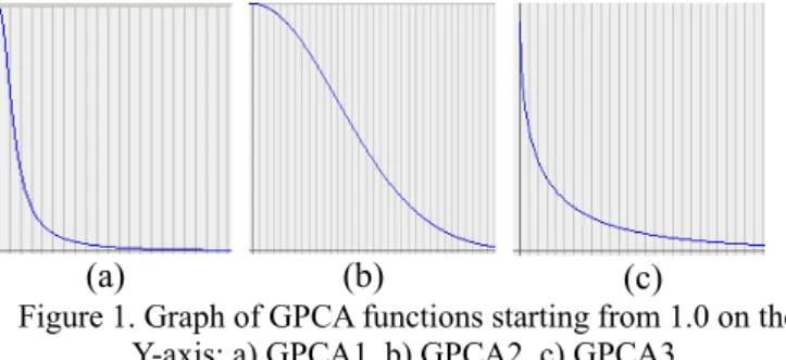
In this paper, three GPCA membership functions were utilized. The functions are based on similar functions used in [3] but were modified to work within the range of the maximum color distance between two pixels. The graphs of the functions are shown in Figure1.
GPCA1: uij = 1 / ( 1 + 0.5 * || xj – vi || 2 ) (9) GPCA2: uij = 2 (-0.005 * || xj – vi || 2) (10) GPCA3: uij = exp{ -1* ( 0.5 || xj – vi || )0.5 } (11) Since the Euclidean distance range between RGB values is only [0, 441.673] the above membership functions will work even if they do not necessarily meet all the constraints.
(a) (b) (c)
Figure 1. Graph of GPCA functions starting from 1.0 on the Y-axis: a) GPCA1, b) GPCA2, c) GPCA3.
2.2 Optimization Algorithms: Particle Swarm Optimization
Swarm intelligence is an artificial intelligence technique in which a population of independent simple agents interacts to produce a global behavior. The methods are based on simulations of wildlife such as birds flocking and fish schooling and on techniques from genetic algorithms and evolutionary programming [4]. The seemingly intelligent behavior of a swarm can be summed by the phrase, "the whole is greater than the sum of its parts." Each agent of a swarm, by itself is not very intelligent. However, when acting together as a group, they can successfully solve complicated problems. One key principle of swarm intelligence is that no leadership is required for the swarm to operate. The agents themselves merely follow simple rules and act on a shared information.
Particle swarm optimization is a type of swarm intelligence algorithm where the agents known as particles attempt to optimize a fitness function by moving through a search space. Early work that developed the functions of PSO can be seen in [4]. PSO, like other forms of swarm intelligence, is a way to simulate social behavior to accomplish a task.
To initialize the algorithm the number of particles is chosen for the swarm. The fitness function is preset, the velocity for each particle is set, and an initial random solution is chosen for each particle. This initial solution of a particle is also their current personal best solution. Each particle's personal best solution is compared to determine the overall best solution found so far. This overall best solution is known as the global best solution. Next, the particles are set in motion by iteratively updating each particle's current solution by using a velocity function. The velocity function is based on a particle's current velocity, its personal best (pBest) solution, and the global best (gBest) solution of all the particles. The velocity function is an attempt to leverage the best information obtained so far against the personal information a particle has obtained itself. The velocity v of particle x is set by this formula:
(12)
where c1 and c2 are user defined constants called the acceleration coefficients, r1 and r2 are random numbers between (0,1), xi represents the current solution of particle x that is under investigation, yi is its personal best solution, and ŷi is the global best solution. Note the
c values in this function are not related the number of clusters. They are used to balance the search between local and global areas of interest. Often they are simply set to the same value. The velocity of the particle has three factors:
o viacts as momentum to help the particle search in new areas.
o c1 * r1 * (yi – xi) is referred to as the "cognitive
component" and it directs the particle back to its personal best solution.
o c2 * r2 * (ŷi – xi) is referred to as the "social
component" and it directs the particle toward the best solution found by the swarm.
The next possible solution for particle x is made by simply updating the present solution by adding the new velocity.
xi (t+1) = xi + vi (t+1) (13) by adding the velocity to the current solution, a particle might overshoot its intended target, but that lets the particle explore new areas of the search space. The success of the PSO depends on the balance of searching new areas versus further investigating known regions of good solutions. The PSO algorithm stops either after a maximum number of total iterations is reached or a set number of iterations is completed where gBest does not change (gBest iteration limit), whichever happens first.
Another key to having a successful PSO is in choosing a fitness function that can accurately measure each result and judge its superiority within a reasonable amount of time. For the experiments, this fitness function was chosen: ⎪ ⎪ ⎪ ⎪ ⎭ ⎪⎪ ⎪ ⎪ ⎬ ⎫ ⎪ ⎪ ⎪ ⎪ ⎩ ⎪⎪ ⎪ ⎪ ⎨ ⎧ + ⎟ ⎟ ⎟ ⎠ ⎞ ⎜ ⎜ ⎜ ⎝ ⎛ − ∑ ∑ ∑ ∑ = c i x x x j i j j j v x 1 1 1 1 max (14)
where x is a pixel, c is the number of clusters, v is the cluster centroid, and xjЄci. This function maximizes the sum of total pixels in a cluster divided by the mean distance of the pixels to the cluster center plus 1. The function attempts to get the largest clusters of pixels that are the shortest average distance from the centroid.
Other possible fitness functions for clustering are: f(xi , Z ) = w1
d
max (Z , xi) + w2 ( z max – d min xi)) (15)))
(
)
(
ˆ
)(
(
))
(
)
(
)(
(
)
(
)
1
(
t
v
it
c
1r
1t
y
it
x
it
c
2r
2t
y
it
x
it
i+ =
+
−
−
v
+
which is recommended by [5]. Where x is a particle, Z is the matrix assignment of pixels to clusters, w1 and w2 are user defined constants, and dmax , dmin are :
max
d
(Z , xi ) = ⎪⎭ ⎪ ⎬ ⎫ ⎪⎩ ⎪ ⎨ ⎧ ∈∑
∀ = zp Cij ij ij p Nc j C m z d( , )/max
1,..., (16)Therefore, dmax is the maximum Euclidean distance of particles to their clusters. Where Nc is the number pixels in clusters, Cij is the pixels that belong to cluster j, |Cij| is the cardinality of set Cij , and mij is the jth cluster centroid vector of the ith particle.
dmin(xi )=
min
{d(m 2 1 2 1j,j j j ≠ ∀ ij1 , mij2)} (17) Thus, dmin is the minimum Euclidean distance between any pairs of clusters.This fitness function attempts to minimize the distance between pixels and their clusters while maximizing the distance between the clusters. An update to this fitness function is given in [6]. It is:
f(xi , Z ) = w1
d
max (Z , xi)+w2 ( zmax – dmin(xi))+w3Je,i(18)
where w3Je,ihas been added to the function of (15). This
new addition is an attempt to minimize the quantization error, Je where w3 is a user defined constant and Je is defined as:
[
]
c N j z C p j j eN
C
m
z
d
J
c j p∑ ∑
= ∀ ∈=
1(
,
)
(19) where(
)
∑
(
)
= − = Nb k pk jk j p m z m z d 1 2 , (20)Various other techniques and parameters can be incorporated into the standard PSO algorithm. An overview of them is given by [7].
There are a few things to consider when choosing the number of particles to use for the PSO. It would seem that more particles are better and thus to set the number of particles to a high number would be better. However, remember that it will take a lot of processing time to run the optimization with a large swarm. Since each particle is independent it will need to spend time processing the fitness function and judging its solution. Therefore, each time the number of particles doubles so does the processing time of the PSO. Hence, for the best performance of PSO in relation to time, it is wise to find the smallest number of particles that can solve the problem effectively. This may be easier said than done, so incrementing the number of particles slowly over several sets of runs should give some evidence if
increasing the number of particles is valuable. If after setting the number of particles to increasingly larger values without useful results, the fitness function may need to be reexamined to determine its merit for the task.
3. Particle Swarm Optimization and
Unsupervised Clustering Algorithms
3.1 Hybrid PSO and Fuzzy Clustering Algorithms: PSO Method 1
The first approach used to combine PSO with a fuzzy clustering algorithm, FCM, PCA, or GPCA, is to first run the fuzzy algorithm to completion. Then, initialize one particle of the PSO with the found solution from the fuzzy clustering algorithm. The reasoning for this procedure is that the fuzzy algorithm is likely to find a good solution. However, it might not always find the optimal solution and sometimes it will find a poor solution. Therefore, if the fitness function of the PSO is well suited to the clustering task it should improve non-optimal solutions while preserving any currently discovered optimal solutions. The fitness function (14) that was developed for these image segmentations was used.
One drawback with this method is that it is giving up some of its initial particle diversity to concentrate on improving a solution. Therefore, this method will likely work best when the fuzzy clustering algorithm finds a near optimal solution that can be improved upon. A fuzzy clustering algorithm that finds many poor solutions should also be helped by this method. However, it seems unnecessary to use processing time to initially run that algorithm when just starting with a random solution would be better and faster.
Hybrid PSO Algorithm: PSO Method 1
Step 0 Run algorithm ai to completion, in order to get the centroids of its solution.
Step 1 Initialize PSO's number of particles, iteration
counter t = 0, gBest counter g = 0.
Step 2 Initialize each particle to a set of random
centroids as their current solution, except set particle x0 to the solution from ai that was calculated in Step 0.
Step 3 Compute fitness of xiand determine yi for all i.
Step 4 Determine ŷi (t+1) , if ŷi (t+1)≠ ŷi (t) then g = 0 else increment g by one.
Step 5 Compute velocity vi (t+1) for all i.
Step 6 Compute yi for all xi.
Step 7 Increment t by one.
Step 8 Repeat steps 3-7 until t = max0 or g = max1.
Step 9 Segment the image using ai utilizing the centroid solution from gBest.
The PSO initializes one particle to the fuzzy clustering algorithm's found solution. It then initializes the rest of the swarm to a random solution for each particle. An iterative loop begins where the fitness of each particle's current solution is calculated using function (14). The gBest solution is saved and then the velocities of the particles are updated using function (12). The iterative loop ends when either the set maximum number of iterations is reached or the gBest solution has no changes in a set number of iterations, whichever happens first.
3.2 Hybrid PSO and Fuzzy Clustering Algorithms: PSO Method 2
In this method, the PSO and the fuzzy clustering algorithm are combined into a single new algorithm. It differs from PSO Method 1 in that the fuzzy clustering algorithm is not run unaccompanied to initialize a single particle of PSO. All of the particles of this PSO are initialized to random solutions. The fuzzy clustering algorithm is only accessed by the PSO for evaluation of the fitness of a solution and for the final segmentation result. Thus, besides the initialization, the behavior of this PSO is the same as in the first method. Similarly, with this PSO method, the same fitness function (14) is utilized. The algorithm for PSO Method 2 is summarized below:
Hybrid PSO Algorithm: PSO Method 2 Step 0 Choose algorithm ai
Step 1 Initialize PSO's number of particles, iteration
counter t = 0, gBest counter g = 0.
Step 2 Initialize each particle to a set of random
centroids as their current solution.
Step 3 Compute fitness of xiand determine yi for all i.
Step 4 Determine ŷi (t+1) , if ŷi (t+1)≠ ŷi (t) then g = 0 else increment g by one.
Step 5 Compute velocity vi (t+1) for all i.
Step 6 Compute yifor all xi.
Step 7 Increment t by one.
Step 8 Repeat steps 3-7 until t = max0 or g = max1.
Step 9 Segment the image using ai utilizing the centroid solution from gBest.
The PSO Method 2 initializes the entire swarm of particles to random solutions. An iterative loop begins where the fitness of each particle's current solution is calculated using function (14). The gBest solution is saved and then the velocities of the particles are updated using function (12). The iterative loop ends when either the set maximum number of iterations is reached or the
gBest solution has no changes in a set number of iterations, which ever happens first.
The value of this method is that the PSO can start running immediately. In addition, given that, the PSO Method 1 will probably judge the initialized particle from the fuzzy clustering algorithm's solution to be the initial gBest, it might lead the PSO away from better solutions. Since an initial poor solution might lead to a premature convergence on a sub-optimal solution, PSO Method 2 should work better than PSO Method 1with the fuzzy clustering algorithms that do not find a near optimal solution.
Unlike PSO Method 1, PSO Method 2 does not have a built-in way to judge the overall improvement in image segmentations. Therefore, the number of good image segmentations produced by PSO Method 2 will be compared to the amount produced by a fuzzy clustering algorithm running by itself. One drawback to this comparison is the random nature of initialization and the algorithms themselves may lead to overestimating or underestimating the success of the method. Therefore, only a significant increase in the number of good segmentations should be considered successful when judging the effectiveness of PSO Method 2.
4. Experiments
4.1 Cluster Validity and Accuracy Assessment
Evaluating the correctness of image segmentation can be open to interpretation. Given a set of images, humans will often segment the same image in several different ways. Good examples of this can be seen in the segmentation of [9]. However, there are scientific approaches to measure image segmentations. Among them are the use of validity indexes and the accuracy of the segmentation as compared to the ground truth of an image.
There are several indexes that attempt to evaluate the quality of segmentation. They rely on statistical facts, such as clusters that are compact and are far from other clusters are considered better than clusters that do not have these properties. The Davies-Bouldin index [10] is one such validity measure commonly used in clustering. To keep the evaluation simple, the Xie-Beni validity index which was developed for the fuzzy measure is not used in this project.
Depending on the nature of the image and the goal of the segmentation there may be in fact a correct segmentation. For example, one such case would be segmenting tumors and normal brain tissue. If a correct segmentation is known a priori for an image this segmentation is often referred to as the ground truth. The final output is a color-coded segmentation of the original image, where each different color represents a cluster.
4.1.1 Davies Bouldin Index
The Davies-Bouldin index is one of several indexes that attempt to gauge the validity of segmentation. Its function, given below, is the ratio of the sum of within cluster distances compared to the distance between the clusters. In this function, for a good result, we want a minimum and maximum distance between clusters. The overall result of the index is that a lower value is a better segmentation than a higher value.
( )
( )
⎭
⎬
⎫
⎩
⎨
⎧
Δ
+
Δ
∑
= ≠(
,
)
max
1
1 k l l k c k l kC
C
C
C
c
δ
(21)The values ∆(C) is the intra-cluster distance. While δ(Ck,
Cl ) is the inter-cluster distance and c is the number of
clusters.
One use for the Davies-Bouldin index is to verify that the number of clusters chosen for an image is optimal. In Figure 2, the three images that are used in the experiments are shown with their Davies-Bouldin index values over several clusters. These values were calculated by running each image against the FCM algorithm for 20 runs per number of clusters. Then, the 10 best Davies-Bouldin index values per image for each number of clusters were averaged to get the value represented on the chart. The Beach and Window image were optimal at 3 clusters and the Shapes image was optimal at 4 clusters. Note that the Shapes image was only slightly better at 4 clusters, while the Beach and Window images were clearly best at 3 clusters. Also, notice that 2 clusters were considered very poor for all images. The Davies-Bouldin index values for 2 clusters was over 30 for each image and therefore does not fit on the chart. 2 3 4 5 6 Beach Window Shapes 0 0.25 0.5 0.75 1 Inde x V a lue Number of Clusters Davies-Bouldin Index Beach Window Shapes
Figure 2. Davies-Bouldin index used to verify number of clusters in an image.
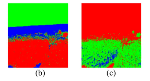
The Davies-Bouldin index can also be used to verify the accuracy of the segmentation. As an example, the Beach image in Figure 3 (b) and (c) were segmented into 3 clusters. Using the Euclidean distance between the
centroids of the clusters and the average Euclidean distance between the pixels and the centroids, Figure 3(b) has a Davies-Bouldin index value of 0.31 and Figure 3(c) has a value of 0.92. The original unsegmented Beach image is shown in Figure 3(a).
Figure 3. (a) the original image and comparing the Davies-Bouldin index value of two segmented images (b)
is better than (c).
The Davies-Bouldin index was accurate in verifying most segmentations. In experiments with this index, it did occasionally give a poor value for a good segmentation. This can happen because many different sets of centroids can give roughly the same segmentation. In an experiment with 100 segmentations of the Beach image from Figure 3(a), the average Davies-Bouldin index value for the 92 good segmentations was 0.35, while the 8 poor segmentations had an average index value of 0.91. However, 3 of the good segmentations had a value that was in between the lowest and highest poor segmentation value. Note that this result is not a failure of the index; instead, it is related to the nature of the fitness function used in the PSO methods. Therefore, it was chosen to visually inspect each segmentation result to guarantee its validity.
4.1.2 Ground Truth
The ground truth of an image represents the correct segmentation of the image based on the segmentation goal. It can be used to evaluate how well the algorithm is working on a particular image or set of images. A pixel-by-pixel comparison of the ground truth image to the algorithm's output segmentation can assign a measured accuracy to the algorithm's clustering ability.
To do this comparison, make a square matrix and an error matrix, equal in size to the number of clusters. Use each column to represent a single cluster. On the diagonals of the matrix, label the number of correct pixel classifications for each column that refers to the ground truth cluster. Use the non-diagonal elements of the matrix to fill in the totals of the number of pixels that were incorrectly classified as
another cluster.
Example error matrix E(r):
(22) ⎟ ⎟ ⎟ ⎠ ⎞ ⎜ ⎜ ⎜ ⎝ ⎛ = cc c c e e e e r E ... ... ... ... ... ) ( 1 1 11
The overall accuracy is obtained by simply summing the diagonals of the error matrix and dividing by the total number of pixels, n.
n e r c i ii
∑
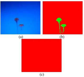
= = 1 ) ( μ (23)However, these measurements should be interpreted carefully. For example, an image with one dominant cluster, as in Figure 4(a), can lead to the segmentation in Figure 4(c) being over 97 percent correct, even though the segmentation should be considered poor.
The error matrix can also be used to determine the real number of clusters produced by the segmentation. If a column of the matrix contains all zeros then that cluster is not represented in the final segmentation. An error matrix with just one column of non-zero values is going to be a poor segmentation. However, even a segmentation with good accuracy and all clusters represented can be judged as having an overall poor segmentation. For example, if Figure 4(c) had a few pixels labeled as the second cluster instead of none. Therefore, when using ground truth as an accuracy measure one should also visually inspect the final segmentations to check the correctness.
(a) (b)
(c)
Figure 4.a) An original image, b) the ground truth data, c) a segmentation with over 97% validity as compared to ground
truth.
For the experiments, all the resulting segmentations were visually checked to verify the accuracy of the clustering. A simple system was devised to classify each resulting segmentation. The segmentation was either
good, in that the result is close to the ground truth image in overall accuracy or it was poor. Each segmentation output image of the fuzzy clustering algorithms was judged before and after it underwent the PSO Method 1. The validity values assigned to an image before PSO were either "good" or "poor". The values assigned after PSO were either "Still Good" (if the previous clustering was good and the current clustering is good.), "Improved to Good" (if the current clustering is now good and the previous clustering was poor), and "Poor, rating not changed" (if the previous clustering was poor and the current clustering is poor). Note that the new segmented images after PSO Method 1 in "Still Good" and "Poor, rating not changed" were not necessarily an exact replica of the previous image, they just were judged to be in the same category. For PSO Method 2, the segmentations were only judged to be "good" or "poor".
4.2 Experimental Results
For the experiments, a graphical Java based program was used to load the images and run the algorithms. The general settings used were fuzzifier, m = 2, maximum number of iterations per algorithm = 40, and the sensitivity threshold = 0.005. For PSO, these values were set: c1 = 2, c2 = 2, and gBest iteration limit = 20. Each algorithm was run 100 concurrent times on each image for a set number of particles. For PSO Method 1, the experiments on the Shapes image were run with 5, 10 and 20 particles. For the Beach and Window images, PSO Method 1 experiments were run with the number of particles set at 5, 10, 20, and 30. For PSO Method 2, all the images were run with 20 particles. All of the fuzzy clustering algorithms' initial centroids were initialized to random values, except PCA93. The PCA93 algorithm did not work well with image segmentation when the initial centroid values were selected at random. It mainly produced only one cluster such as seen in Figure 4 (c). Since this algorithm seemed sensitive to the initial values, it was initialized every time with output centroids from a new FCM run.
The first image, Shapes (320 x 370 pixels), 5(a) is made up of 19 colors; 1 black; 7 mostly blue; 5 mostly green; 6 mostly red and can be divided into 4 clusters just based on the colors of the pixels, 5(b). The second image, Beach (375 x 500 pixels), 6(a) is 77,940 colors. It can be divided into 3 cluster based on color, those being: ocean and sky (blue); sand (light grey); plant life (green), 6(b). The third image, Window (247 x 480 pixels), Figure 7(a) is composed of 15,431 colors. It can be divided into 3 clusters based on color, those being: wall (green); windowpanes (white); glass looking outside (black), 10(b).
Beach is seen in Figure 6(c). The segmentation does have some of the sky mixed up with sand and plants but overall it is good and is 95% accurate to the ground truth image. A good image segmentation of Window is shown in Figure 7(c). The segmentation does have some of the wall mixed up with the window glass and pane but overall it is good and is 99% accurate to the ground truth. For the Shapes image, we only accepted segmentations as good that matched the ground truth 100%. For comparison, some poor segmentations generated by the algorithms are shown in Figures 8, 9 and 10. These poor segmentations were later improved to good by PSO. Note that there were hundreds of poor segmentations that were improved to good. Thus, the figures represent only a very small sample.
(a) (b)
Figure 5. a) Shapes original image and b) shapes ground truth.
(a) (b)
(c)
Figure 6.a) Beach original image, b) beach ground truth , and c) beach typical good segmentation.
(a) (b)
(c)
Figure 7.a) Window original image, b) window ground truth, and c) window typical good segmentation.
(a) (b) (c)
(d) (e)
Figure 8. Some poor segmentations of shapes that were later improved to good by PSO. These images were generated by a)
FCM, b) PCA93, c) GPCA1, d) GPCA2, and e) GPCA3.
(a) (b)
(c) (d)
(e)
Figure 9.Some poor segmentations of beach that were later improved to good by PSO. These images were generated by a)
(a) (b)
(c) (d)
(e)
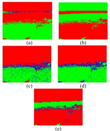
Figure 10. Some poor segmentations of window that were later improved to good by PSO. These images were generated by a)
FCM, b) PCA93, c) GPCA1, d) GPCA2, and e) GPCA3.
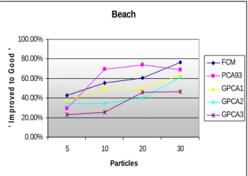
The total result from all the experiments with PSO Method 1 is summarized in Table 1, Table 2, and Table 3 for the Shapes, Beach, and Window images respectively. The PSO algorithm improved about 68% of the poor segmentations overall for the Shapes image, 45% overall for the Beach image, and 47% overall for the Window image. A graph is provided that displays the improvement versus the number of particles used for the PSO in Figure 11, Figure 12, and Figure 13 for the Shapes, Beach, and Window images, respectively. Note in some cases the percent went down slightly as the number of particles increased but this can be attributed to the random nature of the PSO and the clustering algorithms versus the number of runs. For the Shapes image, the results did not vary considerably enough to use 20 instead of 10 particles, except for when using the FCM algorithm. The Windows image did not do considerably better with 30 particles, so 20 particles is adequate for this image. The Beach image, set at 30 particles was preferable for most algorithms except PCA93 and GPCA3, where 20 particles were sufficient for improvement. In addition, even 5 particles helped all the algorithms to improve the overall number of good segmentations. The measured improvement of using only 5 particles was similar to the results from 10 particles on several of the images and algorithms.
Table 1. Summary of the results on Shapes image after running PSO Method 1 Algor- ithm Image Number of Particles Still Good Impr- oved to Good Poor, Rating Not Changed Total Exper-iments Percent changed from poor to good FCM Shapes 5 82 13 5 100 72.22% FCM Shapes 10 85 11 4 100 73.33% FCM Shapes 20 84 16 0 100 100.00% PCA93 Shapes 5 0 11 89 100 11.00% PCA93 Shapes 10 0 14 86 100 14.00% PCA93 Shapes 20 0 12 88 100 12.00% GPCA1 Shapes 5 12 64 24 100 72.73% GPCA1 Shapes 10 10 83 7 100 92.22% GPCA1 Shapes 20 13 81 6 100 93.10% GPCA2 Shapes 5 2 77 21 100 78.57% GPCA2 Shapes 10 0 92 8 100 92.00% GPCA2 Shapes 20 0 93 7 100 93.00% GPCA3 Shapes 5 2 75 23 100 76.53% GPCA3 Shapes 10 2 90 8 100 91.84% GPCA3 Shapes 20 4 87 9 100 90.63% All All 296 819 385 1500 68.02% Shapes 0.00% 20.00% 40.00% 60.00% 80.00% 100.00% 5 10 20 Particles ' Im p ro v e d t o G o o d " FCM PCA93 GPCA1 GPCA2 GPCA3
Figure 11. Shapes image improvement vs. number of particles in PSO Method 1. Beach 0.00% 20.00% 40.00% 60.00% 80.00% 100.00% 5 10 20 30 Particles ' I m p rov e d t o G ood " FCM PCA93 GPCA1 GPCA2 GPCA3
Figure 12.Beach image improvement vs. number of particles in PSO Method 1.
Table 2. Summary of the results on Beach image after running PSO Method 1. Algor- ithm Image Number of Particles Still Good Impr-oved to Good Poor, Rating Not Changed Total Exper- iments Percent changed from poor to good FCM Beach 5 72 12 16 100 42.86% FCM Beach 10 71 16 13 100 55.17% FCM Beach 20 72 17 11 100 60.71% FCM Beach 30 66 26 8 100 76.47% PCA93 Beach 5 32 20 48 100 29.41% PCA93 Beach 10 74 18 8 100 69.23% PCA93 Beach 20 69 23 8 100 74.19% PCA93 Beach 30 71 20 9 100 68.97% GPCA1 Beach 5 22 29 49 100 37.18% GPCA1 Beach 10 19 40 41 100 49.38% GPCA1 Beach 20 20 40 40 100 50.00% GPCA1 Beach 30 21 50 29 100 63.29% GPCA2 Beach 5 18 28 54 100 34.15% GPCA2 Beach 10 25 26 49 100 34.67% GPCA2 Beach 20 25 30 45 100 40.00% GPCA2 Beach 30 25 46 29 100 61.33% GPCA3 Beach 5 17 19 64 100 22.89% GPCA3 Beach 10 21 20 59 100 25.32% GPCA3 Beach 20 26 34 40 100 45.95% GPCA3 Beach 30 25 35 40 100 46.67% All All 791 549 660 2000 45.41%
Table 3. Summary of the results on Window image after running PSO Method 1.
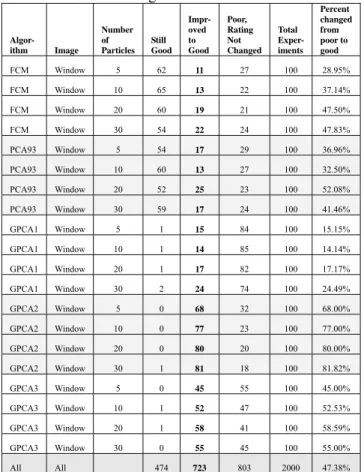
Algor- ithm Image Number of Particles Still Good Impr- oved to Good Poor, Rating Not Changed Total Exper-iments Percent changed from poor to good FCM Window 5 62 11 27 100 28.95% FCM Window 10 65 13 22 100 37.14% FCM Window 20 60 19 21 100 47.50% FCM Window 30 54 22 24 100 47.83% PCA93 Window 5 54 17 29 100 36.96% PCA93 Window 10 60 13 27 100 32.50% PCA93 Window 20 52 25 23 100 52.08% PCA93 Window 30 59 17 24 100 41.46% GPCA1 Window 5 1 15 84 100 15.15% GPCA1 Window 10 1 14 85 100 14.14% GPCA1 Window 20 1 17 82 100 17.17% GPCA1 Window 30 2 24 74 100 24.49% GPCA2 Window 5 0 68 32 100 68.00% GPCA2 Window 10 0 77 23 100 77.00% GPCA2 Window 20 0 80 20 100 80.00% GPCA2 Window 30 1 81 18 100 81.82% GPCA3 Window 5 0 45 55 100 45.00% GPCA3 Window 10 1 52 47 100 52.53% GPCA3 Window 20 1 58 41 100 58.59% GPCA3 Window 30 0 55 45 100 55.00% All All 474 723 803 2000 47.38% Window 0.00% 20.00% 40.00% 60.00% 80.00% 100.00% 5 10 20 30 Particles ' Im p ro v e d t o G o o d " FCM PCA93 GPCA1 GPCA2 GPCA3
Figure 13. Window image improvement vs. number of particles in PSO Method 1.
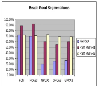
The results of segmentations completed using PSO Method 2 can be seen in Table 4. Again, 100 segmentations were done on each image. A comparison of PSO Method 2, PSO Method 1, and just running the fuzzy clustering algorithms alone can be seen in Table 5. The comparison summarizes the percent of total good segmentations each algorithm produced on each image. This data is also displayed graphically for the Shapes, Beach, and Window images in Figure 14, Figure 15, and Figure 16, respectively.
For the Shapes image, PSO Method 1 and PSO Method 2 had nearly identical performances and did better than just running the fuzzy clustering algorithms without PSO. On the Beach image, PSO Method 1 did better than PSO Method 2 when the fuzzy clustering algorithm itself had more good segmentations. However, PSO Method 2 did better when the fuzzy clustering algorithm was not as suited to segmenting the image correctly. On the Window image, the PSO Method 2 did best overall. However, the number of good segmentations was very similar to PSO Method 1 when the image could be accurately segmented by these fuzzy clustering algorithms.
Overall, there was more than double the number of good segmentations produced by either the PSO Method 1 or the PSO Method 2 than by just running the fuzzy clustering algorithm alone.
Table 4. Summary of Results when using Algorithm + PSO Method 2. Algorithm + PSO Method 2 Image Number of Particles Good Segmentations Poor Segmentations Total Experiments FCM Shapes 20 93 7 100 PCA93 Shapes 20 19 81 100 GPCA1 Shapes 20 94 6 100 GPCA2 Shapes 20 92 8 100 GPCA3 Shapes 20 96 4 100 FCM Beach 20 72 28 100 PCA93 Beach 20 71 29 100 GPCA1 Beach 20 73 27 100
GPCA2 Beach 20 69 31 100 GPCA3 Beach 20 69 31 100 FCM Window 20 84 16 100 PCA93 Window 20 79 21 100 GPCA1 Window 20 86 14 100 GPCA2 Window 20 90 10 100 GPCA3 Window 20 86 14 100 All All 20 1173 327 1500
Table 5.Good segmentations produced by PSO Method 1 and Method 2 vs. Non-PSO algorithm.
Algorith m Image Number of Particles No PSO PSO Method 1 PSO Method 2 Experime nts Each Method FCM Shapes 20 84 100 93 100 FCM Beach 20 72 89 19 100 FCM Window 20 60 79 94 100 PCA93 Shapes 20 0 12 92 100 PCA93 Beach 20 70 92 96 100 PCA93 Window 20 52 77 72 100 GPCA1 Shapes 20 13 94 71 100 GPCA1 Beach 20 20 60 73 100 GPCA1 Window 20 1 18 69 100 GPCA2 Shapes 20 0 93 69 100 GPCA2 Beach 20 25 55 84 100 GPCA2 Window 20 0 80 79 100 GPCA3 Shapes 20 4 91 86 100 GPCA3 Beach 20 26 60 90 100 GPCA3 Window 20 1 59 86 100 All All 428 1059 1173 1500
Shapes Good Segmentations
0.00% 10.00% 20.00% 30.00% 40.00% 50.00% 60.00% 70.00% 80.00% 90.00% 100.00%
FCM PCA93 GPCA1 GPCA2 GPCA3
No PSO PSO Method 1 PSO Method 2
Figure 14. Shapes image percent of "Good" segmentations produced by each method.
Beach Good Segmentations
0.00% 10.00% 20.00% 30.00% 40.00% 50.00% 60.00% 70.00% 80.00% 90.00% 100.00%
FCM PCA93 GPCA1 GPCA2 GPCA3
No PSO PSO Method1 PSO Method2
Figure 15. Beach image percent of "Good" segmentations produced by each method.
Window Good Segmentations
0.00% 10.00% 20.00% 30.00% 40.00% 50.00% 60.00% 70.00% 80.00% 90.00% 100.00%
FCM PCA93 GPCA1 GPCA2 GPCA3
No PSO PSO Method1 PSO Method2
Figure 16.Window image percent of "Good" segmentations produced by each method.
Based on the results of the previous section, there is enough evidence to suggest that adding a PSO algorithm after or along with fuzzy clustering can improve the total positive results. The outcomes for the hybrid PSO methods were positive for both fuzzy clustering algorithms that segmented an image initially well and ones that did not. Depending on the image and the initial algorithm, the PSO Method 1 algorithm added at least a 10% improvement to the algorithms that were better suited to a particular image. The PSO Method 2 algorithm did as well as the standalone fuzzy clustering algorithm and was better than PSO Method 1 in several cases.
Both PSO Method 1 and PSO Method 2 were very comparable in accuracy in segmenting the test images. In general, PSO Method 1 seemed to have an edge when
the fuzzy clustering algorithm could at least segment the image correctly 70% of the time. Conversely, PSO Method 2 was better when the fuzzy clustering algorithm was not that accurate. This disparity can only be attributed to the particle initialization of the algorithms since that is the only difference between the two methods.
However, the improvement in the segmentation comes with the trade-off of longer processing times. Running a PSO can add a considerable amount of running time to the segmentation. Within the PSO itself, the processing time is effectively doubled with the doubling of the number of particles. Therefore, to reduce this time, the number of particles set should be tailored to the image and the algorithm. A value of 20 particles seemed to do well in general. However, even 5 particles did produce good results and could be used as a starting point for experimentation. The extra time to run PSO could also be mitigated if the PSO was programmed to run in a parallel computing environment. PSO should be well suited to a distributed environment, since the particles are independent agents and only rely on each other for an updated gBest value.
5. Conclusions
In this study, two PSO methods were developed to aid in the segmentation of images by fuzzy clustering algorithms. In total 7,000 experiments were run with promising results. The images were segmented by using only their color feature. All the images consisted of 24-bit color pixels with three 8-bit bytes for Red, Green, and Blue. The resulting data demonstrated that there is certainly room for improvement in the accuracy of the fuzzy clustering algorithms when used for segmenting images. PSO Method 1 was beneficial to all the algorithms no matter which image was being segmented. PSO Method 2 was beneficial to the majority of the algorithms and the images. However, in a few instances it did not produce a significant enough gain in the number of good segmentations to justify the added cost of running it.
Since this study only used the color feature, additional research will need to be done to test the effectiveness of these PSO methods when different features are used. However, adding a PSO in a similar way to the spatial and texture features of more challenging images should have comparable potential because of the flexibility of PSO. One good characteristic of the PSO is its adaptability to different problems by simply changing the fitness function. This validity measure is the key to a successful PSO and it needs to be tailored to the subject matter. Nonetheless, it can also be a daunting task to make a function that is both accurate and reasonable in
its running time. The down side of PSO, namely the running times, could be alleviated if it was coded to run on a distributed or parallel system. However, on a sequential machine, if processing time is a concern, then a small number of particles could be used. As this research indicates, even a PSO with as little as 5 particles can produce good results.
Both methods of PSO used did well overall in helping to segment the images correctly. However, PSO Method 1 was better suited to work with algorithms that could accurately segment an image 70% of the time, while PSO Method 2 was generally better suited to algorithms that did not segment the image correctly as often. These characteristics of the methods could be attributed to the initial diversity of the solution (swarm) population. Whereas in PSO Method 1, if an initial solution is already near optimal, more diversity is not needed to fine tune it. However, the results of PSO Method 2 show that it is better to have no previous solution than to have a misguided one.
The general PSO algorithm does not offer many ways, besides the fitness function, to adjust its clustering characteristics. However, one way to add diversity without adding more particles would be to alter the constants c1 and c2 as the PSO is running. In the early stages of PSO the c1 constant could be set larger than c2. As the PSO progresses, c2 could become increasingly larger. This process in effect would mimic the properties of the simulated annealing algorithm, which replicates the heating and controlled cooling used in metallurgy to reduce defects in metal. Therefore, the cognitive component of the particle would have more freedom to explore its personal best solution which should help prevent premature convergence. Adding this feature to PSO Method 1 could help it better perform with the fuzzy clustering algorithms that did not usually segment the images well themselves.
Even though PSO was used only with fuzzy clustering algorithms, the methods described for combining these algorithms with PSO could easily be implemented with other types of clustering algorithms. Also, the methods could be used to optimize the segmentation on other features of images such as spatial and texture.
Acknowledgment
The author, Dr. Liu, would like to thank for research support from Beijing Science and Technology Commission Project (No. Beijing Forestry 0011), National “863” Program of China (No. 2006AA10Z232) and the Beijing Municipal Education Commission Project (No. KM200710009005)
.
References
[1] J. C. Bezdek and P. F. Castelaz, “Prototype Classification and Feature Selection with Fuzzy Sets,” IEEE Transaction on Systems, Man, and Cybernetics, vol. 7, pp. 87-92, 1977.
[2] R. Krishnapuram and J. M. Keller, “A Possibilistic Approach to Clustering,” IEEE Transactions on Fuzzy Systems, vol. 1, no. 2, pp. 98-110, 1993. [3] J. Zhou and C. C. Hung, “A Generalized Approach
to Possibilistic Clustering Algorithms,”
International Journal of Uncertainty, Fuzziness & Knowledge-Based Systems, vol. 15, pp. 110-132, 2007.
[4] J. Kennedy and R. Eberhart, “Particle Swarm Optimization,” Proc. of the IEEE Int. Conf. on Neural Networks, pp. 1942-1948, 1995.
[5] M. Omran, A. Salman, A. P. Engelbrecht, “Image Classification using Particle Swarm Optimization,”
Proc of the 4th Asia-Pacific Conference on Simulated Evolution and Learning, pp. 370-374, 2002.
[6] M. Omran, A. Salman, A. P. Engelbrecht, “Particle Swam Optimization Method for Image Clustering,”
International Journal on Pattern Recognition and Artificial Intelligence, vol. 19, iss. 3, pp. 297- 322, 2005.
[7] F. Van Den Bergh and A.P. Engelbrecht, “A Study of Particle Swarm Optimization Particle Trajectories,” Information Sciences, vol. 176, no. 8, pp. 937-971, 2006.
Chih-Cheng Hung received his B.S. in
business mathematics from Soochow University in Taiwan, and his M.S. and Ph.D. in Computer Science from the University of Alabama in Huntsville, AL in 1986 and 1990, respectively. He is a professor in Computer Science at Southern Polytechnic State University, GA. He was with the Department of Image Processing Applications at Intergraph Corporation to develop image processing software tools from 1990 to 1993. He is the co-chair for the 20th Association of Computing Machinery (ACM) Symposium on Applied Computing (SAC) – Computational Intelligence and Image Analysis Track being held in Honolulu, Hawaii, USA from March 8 to 12, 2009. He is an associate editor of Information: An Intenational Interdisciplinary Journal. His research interests include image processing, pattern recognition, neural networks, genetic algorithms, artificial intelligence and software metrics.
[8] K. S. Chuang, H. L. Tzeng, S. Chen, J. Wu, and T. J. Chen, “Fuzzy C-Means Clustering with Spatial Information for Image Segmentation,”
Computerized Medical Imaging and Graphics, vol. 30, pp. 9-15, 2006.
[9] D. Martin, C. Fowlkes, D. Tal, and J. Malik, “A Database of Human Segmented Natural Images and its Application to Evaluating Segmentation Algorithms and Measuring Ecological Statistics,”
Proc. 8th Int’l Conf. Computer Vision, vol.2, pp. 416-423, 2001.
[10] D. L. Davies and D. W. Bouldin, “A Cluster
Separation Measure,” IEEE Trans. Pattern
Analysis and Machine Intelligence, vol.1, pp. 224-227, 1979.
[11] S. Theodoridis and K. Koutroumbas, Pattern Recognition, 3rd ed., Academic Press, 2006.
Wenping Liu received B.S. and M.S.
degrees in electronics engineering from Xidian University, Xi’an, China, in 1991 and 1996, and a Ph.D. in Computer Science from Fudan University, Shanghai, China, in 1999, respectively. She was a senior research member in IBM China Research Lab from 1999 to 2001. She is currently an associate professor of computer science and information engineering at Beijing Forestry University. She is a SPIE member. Her current research interests include digital image processing, pattern recongnition, fuzzy system, human-computer interaction and mulitmedia retrieval.
Ethan McGrath received his M.S. degree in computer
science from Southern Polytechnic State University, GA in 2007. His research interests include digital image processing, swarm intelligence, optimization techniques, software metrics, artificial intelligence, and mulitmedia retrieval.
Bor-Chen Kuo received B.S. and M.S.
degrees from National Taichung Teachers College, Taichung, Taiwan, in 1993 and 1996, respectively, and a Ph.D. from the school of electrical and computer engineering, Purdue University, West La-fayette, IN, in 2001. He is currently a professor in the Graduate Institute of Educational Measurement and Statistics at the National Taichung University, Taiwan. His research interests are pattern recognition, remote sensing, image processing, and nonparametric functional estimation.