Proteins 2D Structure Prediction from 1D Sequence by Signal Processing and Soft Computing Methods

(1)

Int. J. Adv. Res. Sci. Technol. Volume 4, Issue 1, 2015, pp.389-397.

International Journal of Advanced Research in

Science and Technology

journal homepage: www.ijarst.com

ISSN 2319 – 1783 (Print)

ISSN 2320 – 1126 (Online)

Proteins 2D Structure Prediction from 1D Sequence by Signal Processing and

Soft Computing Methods.

Jayakishan Meher *

Dept. of Computer Science and Engineering, Vikash College of Engineering for Women, Bargarh, Odisha, India.

*Corresponding Author’s E-mail: [email protected]

A R T I C L E I N F O A B S T R A C T

Article history:

Received Accepted Available online

10 Jan. 2015 20 Feb. 2015 25 Feb. 2015

Research in protein structure and function is one of the most important research areas in modern bioinformatics and computational biology. The structure of a protein is related to its function. The information necessary for protein folding resides completely within the primary structure. The development of rapid methods of DNA sequencing coupled with the straightforward translation of the genetic code into protein sequences has amplified the urgent need for automated methods of interpreting these one-dimensional(1D), linear sequences in terms of two-dimensional(2D) structure. There is a considerable room for improvement. In this paper an effective feature extraction method based on discrete wavelet transform (DWT) to detect informative proteins. Support vector machine, Multilayered perceptron (MLP) and radial basis function (RBF) neural network classifiers are used to efficiently to predict the protein secondary structure which aims to classify the three types of α-helix, β-sheet and C-coil. Effective numerical representation based on physico-chemical parameters such as EIIP, polarizabilty, dipole moment and alpha induces the prediction more accurately. The potential of the proposed approach is evaluated through an exhaustive study by benchmark non-redundant dataset and a prediction accuracy of 95% is achieved.

Keywords:

Protein secondary structure , α-Helix,

β-Strand, coils,

Wavelet transform, Support vector machine, Multilayered perceptron.

Introduction:

Molecular biologists have been fascinated with the possibility of obtaining a complete two-dimensional and three-dimensional picture of a protein by simply applying the proper algorithm to a known

one-dimensional amino acid sequence. Determining the

protein structure from amino acid sequence leads to better understanding of the functionality of the protein resulting in faster drug discovery. Proteins are macromolecules that are responsible for a wide range of vital biochemical functions, which include acting as catalysts, oxygen transport, cell signaling, antibody production, nutrient transport and building up muscle fibers [1-2]. More specifically, proteins are chains of amino acids, of which there are twenty different types, joined by peptide bonds. Proteins have a three-level structural hierarchy, typically referred to as primary, secondary and tertiary structure [3]. The higher-level structures determine the function of the protein and consequently, the knowledge of the structure provides insight into its function. Proteins are large polypeptides which consist of 20 amino acid residues. Chemical

properties that distinguish these amino acids cause the protein chains to fold up into specific structures that define their particular functions in the cell.

(2)

www.ijarst.com Manash. et al. Page | 390

of a protein and hydrophilic amino acid chains gather on the outside. Sulphur bridges stabilize the structure. Prediction of the secondary structure is important as it provides insights into the function of the protein. By jointly comparing amino acid and secondary structure sequences, it is possible to improve the prediction of protein function [6]. In addition, secondary structure prediction is a step towards the prediction of the 3-D structure of a protein.

The fundamental elements of the secondary structure of proteins are α-helices, β-sheets, coils and turns. Thus, the secondary structure prediction can be analyzed as typical pattern recognition or classification problem, where the secondary structure class of a given amino acid residue in a protein is predicted based on its

sequence features. α-helices are strengthened by

hydrogen bonds between every fourth amino acid so

that the protein backbone adopts a helical configuration

as shown in Figure 1. Likewise in loops (e.g., turns or bends), the hydrogen bonding is mostly local. For example, the turn segment has a hydrogen bond between the first and the fourth amino acids. The hydrogen bonding structure in β-strands is slightly different, where both local and nonlocal interactions are

observed. In β-strands, the most common local

hydrogen bonding is between every two amino acids, and nonlocal interactions are due to hydrogen bonds between amino acid pairs positioned in interacting β- strand segments [7].

Various statistical, machine learning and signal processing algorithms have been used to predicting the secondary structure of proteins from their amino acid sequences. A simple goal in the secondary structure prediction is to predict whether an amino acid residue of a protein is in a helix, strand or coil [8]. The first generation of secondary structure prediction techniques emerged in the 1960s and were based on single amino acid propensities and, for each amino acid, calculated the probability of it belonging each of the secondary structural elements. The secondary generation of prediction methods extended this concept by taking into account the local environment, of an amino acid, into consideration. Prediction accuracies with the second generation methods seemed to stall at around 60% accuracy, seemingly because these methods were local in that only information in a window of adjacent residues were used in predicting the secondary structure of an amino acid. [9] Local information accounts for approximately 65% of secondary structure information [10]. Since the early 1990s, third generation prediction methods achieved prediction accuracies around 70% and such methods incorporate machine learning techniques, evolutionary knowledge about proteins and with relatively more complex algorithms. [10-11].

Homology modeling bases the prediction for an unknown target protein, on the known secondary structures of proteins of similar amino acid sequence [12]. The basis of threading is that a limited number

of unique protein folds exist in nature and structure prediction of a target sequence can be performed by consulting a database of known folds and determining which fold-model best fits the sequence. Both homology modeling and threading rely on the existence of known structures and the disadvantage of such approaches is that accurate prediction relies on proteins of similar structure already being solved. Another approach, namely the ab initio techniques [13] or prediction from first principles, bases structure prediction on known biochemical and biophysical facts related to the proteins. In general they are computationally very expensive methods. Machine learning methods such as neural network and nearest neighbor techniques, utilize a localized prediction methodology in the sense that a window, typically of less than 20 amino acids, is presented to the prediction system with the aim of predicting secondary structure.

However, local information accounts for

approximately 65% of secondary structure formation [8]. Therefore, prediction can potentially be improved by incorporating a more global prediction scheme [9]. Secondary structure prediction methods often employ neural networks (NNs) [14], SVMs [15], and hidden Markov models (HMMs) [16, 17]. In neural networks and SVMs utilize an encoding scheme to represent the amino acid residues by numerical vectors. On the other hand, in HMM methods, hidden states generate segments of amino acids that correspond to the non-overlapping secondary structure segments. There are two types of protein secondary structure prediction algorithms. A single sequence algorithm does not use information about other similar proteins. The algorithm should be suitable for a nonhomologous sequence with no sequence similarity to any other protein sequence. Algorithms of another type explicitly use sequences of homologous proteins, which often have similar structures. The accuracy (sensitivity) of the best current single sequence prediction methods is below 70%. The prediction accuracy of the best prediction methods that employ information from multiple alignments is close to 82.0% [18].

The genomic and proteomic information are digital in nature and thus makes it suitable for the application of signal processing techniques to better analyze and understand the characteristics of DNA, proteins, and their interaction. Therefore, signal processing offers a variety of methods from pattern recognition and network analysis for the diagnosis and therapy of genetic diseases [19-20]. It is possible to map protein into a digital signal by assigning numeric values to each amino acid. DSP techniques relating to protein structure

analysis assign numeric values - often their

(3)

Int. J. Adv. Res. Sci. Technol. Volume 4, Issue 1, 2015, pp.389-397. methodology that is primarily targeted for any given

query protein rather being trained over a pre-determined training set is used by D. Mitra and M. Smith based on homology-modeling to improve the accuracy [26]. For some query proteins our prediction accuracies are predictably higher than most other methods, while for other proteins they may not be so, but we would at least know that even before running the algorithms. When a significantly homologous protein with known structure is available in the database the prediction accuracy could be even 90% or above. This uses digital signal processing technique that is of global nature in assigning structural elements to the respective residues. An automated approach for the secondary structure prediction based on the Digital Signal Processing (DSP) techniques which involve two DSP operators, Convolution and Deconvolution are used by D. Mitra and M. Smith for the purpose of predicting secondary structures [26]. Mappings between an amino acid sequences and the corresponding numerical time-series or “signals” are processed. Convolution is a method of applying a filter on an incoming signal, producing an outgoing signal. Deconvolution is the inverse operation of convolution and permits the filter to be recovered if the outgoing signal and the incoming signal are known. This method predicts three states (helix, strand, and coil) for the secondary structure.

Secondary structure of a protein can be predicted efficiently by combining continuous wavelet transform (CWT) and Chou-Fasman method. The authors in [27] have selected a protein with ID 1gca from PDB database, and substituted every amino acid of the protein with corresponding hydrophobic value. Then CWT was used to get the nucleated residues of certain type of secondary structure. The regions were extended along the protein sequence in each direction based on Chou-Fasman rules. The prediction accuracy for alpha-helix, beta-sheet, loop is 80% on an average. Support

vector machines (SVM) have shown strong

generalization ability in a number of application areas, including protein structure prediction. In [28] a new tertiary classifier is introduced that makes use of support vector machines as neurons in a neural network architecture. This network is optimized using genetic algorithms. The novel tertiary classifier is better than most available techniques. In [29] Golem takes, as input, examples and background knowledge described as Prolog facts. It produces, as output, Prolog rules which are a generalization of the examples. Golem was applied to learning secondary structure prediction rules for alpha domain type proteins Golem learned a small set of rules predicting which residues is part of α-helices based on their positional relationships and chemical and physical properties. This representation is more easily understood by molecular biologists. Performance of the learned rules was 81%.

The rest of the paper is organized as follows. Section 2 describes materials used for protein secondary structure of proteins. This section includes

dataset preparation and then how to represent the amino acid sequence in numerical sequence. The section 3 describes the proposed method of prediction of secondary structure of proteins. This section includes the wavelet transform based feature extraction and followed by a support vector machine, multi layer perceptron and radial basis function neural network classifier to predict the major classes of secondary structure of proteins. Simulation result has been discussed in section 4 and section 5 draws conclusions.

Materials Used:

A. Dataset Preparation:

Co-ordinate files of proteins are obtained from the protein data bank. For the study in this work we have

chosen a non-redundant set of PDB files. From the

non-redundant PDB chain set and their coordinate files

obtained from the public domain are used for preparing a database of elements of protein secondary structure. Using MAPMAK [30] program the major classes of secondary structure of protein such as α-Helix, β, Turn and Random are found out.

Table 1. Physico-chemical properties of amino acids

Amino acid

EIIP

Polarizability Dipole moment

Alpha

A 0.0373 4.44 5.937 1.489

R 0.0959 14.16 37.5 1.0224

N 0.0036 7.72 18.89 0.772

D 0.1263 6.55 29.49 0.924

C 0.0829 7.44 10.74 0.996

Q 0.0761 11.39 39.89 1.164

E 0.0058 8.38 42.52 1.504

G 0.0050 2.61 0.0 0.510

H 0.0242 11.84 20.44 1.003

L 0.0000 9.95 3.782 1.236

I 0.0000 9.95 3.371 1.003

K 0.0371 10.72 50.02 1.172

M 0.0823 11.11 8.589 1.363

F 0.0946 14.10 5.98 1.195

P 0.0198 8.69 7.916 0.492

S 0.0829 5.08 9.836 0.739

T 0.0941 6.92 9.304 0.785

W 0.0548 19.37 10.73 1.090

Y 0.0516 14.74 10.41 0.787

V 0.0057 8.11 2.692 0.990

B. Numerical Representation of Amino acid Sequence:

(4)

numerical representations, but the methods having high sensitivity and specificity is obtained by using physico-chemical properties of amino acids. It is seen that physico-chemical properties of amino acid residues such as EIIP, polarizability, dipole moment and alpha are correlated with the structure and function of the proteins and hence help in the classification of major classes of protein secondary structure of protein effectively. If we substitute the dipole moments for amino acids, we get a numerical sequence which represents the distribution of polarity of a chemical bond within a molecule along the protein sequence. Now the resulting numerical representation is subjected

for analysis. The amino acid sequence of each character

is converted into numerical sequence by substituting its physico-chemical parameter of residues (Table 1) from a known dataset.

Proposed method of Prediction:

A. Wavelet based feature extraction method:

Protein data is very rich and complex. Such data can be analyzed with wavelet transform to extract the important features. This transformation method is used for feature extraction for a machine learning approach to the protein secondary structure prediction problem.

Recently, the use of wavelet transform in the Bioinformatics field is promising. A wavelet is a waveform that is localised in both time and frequency domains. This wavelet is dilated and translated along the signal to perform the analyses. The commonly used wavelets in practice are Haar, Daubechies, Gaussian wave, Mexican hat and Morlet wavelets. The selection of particular wavelet for any analysis depends on the kind of signal being studied and kind of signal variation to be captured.

An important attribute of wavelet methods is that, due to the limited duration of every wavelet, local variations of the signal are better extracted and information on the location of these local features is retained in the constituent waveforms. In discrete wavelet transform a subset of scales and positions are chosen, in which the correlation between the signal and the shifted and dilated waveforms are calculated. Consequently, the signal is decomposed into several groups of coefficients, each containing signal features corresponding to a group of frequencies. Small scales refer to compressed wavelets, depicted by rapid variations appropriate for extracting high frequency features of the signal.

Wavelet transform has been applied for transmembrane structure prediction [31]. In this work, the wavelet transform is used to determine kink in segments of amino acid sequences of α-helical membrane proteins. Protein sequence similarity has also been studied using DWT of a signal associated with the average energy states of all valence electrons of each amino acid [32]. DWT has been applied on hydrophobicity signals in order to predict hydrophobic

cores in proteins [33].

Wavelet transform proposed by Grossman and

Morlet [34] is an efficient time-frequency

representation method which transforms a signal in time domain to a time-frequency domain. The basic idea is that any signal can be decomposed into a series of dilations and compressions of a mother wavelet (

(t)

 _{). Hence the continuous wavelet transform of a}

signal is defined as:

1

( , ) ( ) t b

CWT a b x t dt

a



 



 

 _ _

 



(1)

,

1

( ) , ,

a b

t b

t a R b R

a a

 _    _  _

 

 

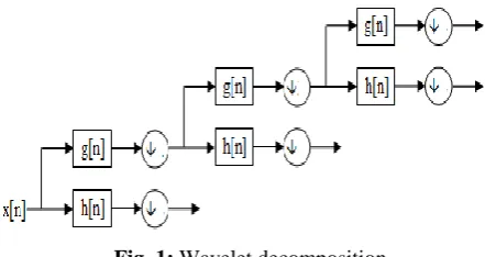
The resolution of the signal depends on the scaling parameter „a‟ and the translation parameter „b‟ determines the localization of the wavelet in time. The CWT can be realized in discrete form through the discrete wavelet transform .The DWT is capable of extracting the local features by separating the components of the signal in both time and scale. In the protein data the amino acid sequence is considered as a signal which can be represented as a sum of wavelets at different time shifts and scales using the DWT.

Fig. 1: Wavelet decomposition

The wavelets can be realized by iteration of filters with rescaling which was developed by Mallat [35] through wavelet filter banks. The resolution of the signal, which is a measure of the amount of detail information in the signal, is determined by the filtering operations, and the scale is determined by up sampling and down sampling operations. The approximation coefficients obtained by the decomposition at a particular level is used as the features for further study. The discriminate feature set has been obtained from discrete wavelet transform into level 2 using db7 wavelet to get the approximation coefficients as the extracted feature set. The Wavelet decomposition is shown in figure 2.

B. SVM Classifier for protein structure:

(5)

output. The feature vectors are mapped into a higher dimensional space Φ(xi) Є H. SVM optimizes separating hyperplane in higher dimensional space as follows:

Min (1/2) wT_{Φ(xj) + C Σξi, where w is a weight factor} Subject to yi(wT_{Φ(xj) + b) ≥ 1 - ξi where ξi ≥ 0}

C > 0 is the penalty factor of the errorterm.

K(xi, xj) = ΦT(xi) Φ(xj) is the kernel function. The

type and parameters of kernel functions are determined after running the training set of feature vectors with known class labels. The kernel parameters resulting in minimum error are selected for prediction in set of feature vectors with known classification to validate the method. Parameters with satisfactory accuracy of prediction are then chosen to design the kernel function for prediction of class in the present case kink in the helix.

A set of feature vectors from each classare taken

as database. These feature vectors are submitted for training. From the training set of kernels the ones with lowest mean square error (MSE) are chosen to validate the kernel. The kernel with highest accuracy is selected for prediction. Separate sets of feature vectors are constructed with several single parameters associated with amino acid residues namely, propensity for alpha helix, beta structure, coil, turn, polarizability, logP, dipole moment, hydropathy index, volume, and hydration energy. This is done to find out if one or more parameters contribute to prediction. The propensity for EIIP and alpha only gives good result.

An anova kernel (MSE = 2.86 E -07) with γ=0.3,

degree = 5, C=0.1, and

ε

= 0.0001gives the best

prediction. Accuracy, Recall and Precision are 80%, and E=20%. SVM method with anova kernel predicts with 85% accuracy. It is a modest beginning to develop a predictor. This could be useful in fine tuning the secondary structure prediction of proteins.

C. MLP neural network classifier for kink prediction:

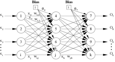
Multi-layer perceptrons (MLP) are used with many applications in data classification. An MLP can be viewed as a logistic regression classifier where the input is first transformed using a learnt non-linear transformation. This transformation projects the input data into a space where it becomes linearly separable [37,38]. The supervised learning process of an MLP with input data and target requires the use of an objective function in order to assess the deviation of the predicted output values from the observed data values and use that assessment for the convergence towards an optimal set of weights. An MLP with a hidden layer can be represented graphically as follows:

Fig. 2: Multi-layer perceptron neural network

When a specified training pattern is fed to the input

layer, the weighted sum of the input to the jth node in

the hidden layer is given by

Net

_j





w

_ij

x

_j





_j (2)

Equation (7) is used to calculate the aggregate input to

the neuron. The

w

_ijterm is the weighted value from

a bias node that always has an output value of 1. The bias node is considered a pseudo input to each neuron in the hidden layer and the output layer, and is used to overcome the problems associated with situations where the values of an input pattern are zero. If any input pattern has zero values, the neural network could not be trained without a bias node. To decide whether a neuron should fire, the Net term, also known as

the action potential, is passed onto an

appropriate activation function. The resulting value from the activation function determines the neuron's output, and becomes the input value for the neurons in the next layer connected to it.

j

Net k

j

e

x

O

_





1

(3)

Since one of the requirements for the Back propagation

algorithm is that the activation function is

differentiable, a typical activation function used is the Sigmoid equation. If the actual activation value of the

output node, k, is Ok. The expected target output for

node k is tk the difference between the actual output and

the expected output is given by



_k



t

_k



O

_k (4)

The error signal for node k in the output layer can be calculated as



_k





_k

O

_k

(

1 

O

_k

)

(6)

where the Ok(1-Ok) term is the derivative of the

Sigmoid function. With the delta rule, the change in the

weight connecting input node j and output node k is

proportional to the error at node k multiplied by the

activation of node j. The formulas used to modify the

weight, wj,k, between the output node, k, and the node, j

is:



w

_j_,_k



l

_r



_k

x

_k

k j k j k

j

w

_,



_,





_, (6)

where ∆Wj,k is the change in the weight between nodes j and k, lr is the learning rate. The learning rate is a relatively small constant that indicates the relative change in weights. If the learning rate is too low, the network will learn very slowly, and if the learning rate

is too high, the network may oscillate

around minimum point. It is desirable to minimize the error on the output nodes over all the patterns presented to the neural network. The following equation is used to calculate the error function, E, for all patterns









 





2

1

k k

O

t

E

(7)

In this work, we use multilayer perceptron as a three-layer feed forward network with weight adjusted by conjugate gradient minimization factor. The perceptron classifies the input vector X into two categories. The perceptron has been trained to return the correct answer on all training examples, and perform well on examples. The MLP has been validated by injecting test dataset and the accuracy was found out to be 91%.

D. Radial basis function neural network classifier:

The main goal of a secondary structure prediction algorithm needs a classifier having a feature set that is comprehensive enough to capture the essential correlations from the available data. Wavelet transform method is used for feature extraction for a machine learning approach to the protein secondary structure prediction problem. For function approximation and pattern classification problems the radial basis function network (RBFNN) has been used in this paper which is a neural structure because of their simple topological structure and their ability to learn in an explicit manner.

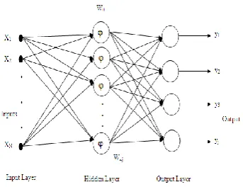
The radial basis function neural network is simple in structure. In the RBF network, there is an input layer, a hidden layer consisting of nonlinear node function, an output layer and a set of weights to connect the hidden layer and output layer. Due to its simple structure it reduces the computational task as compared to conventional multi layer perception (MLP) network. In RBFNN, the basis functions are usually chosen as Gaussian and the number of hidden units are fixed using some properties of input data [39,40]. The structure of a RBF network is shown in Fig. 3.

Fig. 3: The RBFNN based classifier

For an input feature vector x, the output of the jth output node is given as.

k 2 k

x ( n ) C

N N

2

j kj k kj

k 1 k 1

y w w e

 



 





 



(8)

The error occurs in the learning process is reduced by updating the three parameters, the positions of centers

(Ck), the width of the Gaussian function (

σ

k) and the

connecting weights (w) of RBFNN by a stochastic gradient approach as defined below:

w

w(n 1)

w(n)

J(n)

w



 

 



₍₉₎

k k c

k

C (n 1)

C (n)

J(n)

C



 

 



(10)

k k

k

(n 1)

(n)

_



J(n)



  

 



(11) Where

2 1

J(n) e(n)

2



, e (n) =d (n) - y (n) is the error, d (k) is the target output and y (k) is the predicted output.

w



C_And



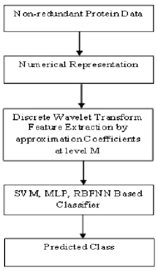
_{are the learning parameters of the}

RBF network. The complete process of the proposed feature extraction based protein secondary structure prediction process is presented in Fig. 4.

Results and Discussion:

All the datasets categorized into multi class to assess the performance of the proposed method. The feature selection process proposed in this paper has two steps. First the protein data is decomposed and optimally choose the discriminate feature set then using discrete wavelet transform into level 2 using db7 wavelet to get the approximation coefficients as the extracted feature set. The performance of the proposed feature extraction method is analyzed with the well studied neural network classifiers such as SVM, MLP and RBFNN.

In order to compare the efficiency of the proposed method in predicting the class of the protein structure we have used standard non-redundant datasets. All the

(7)

α-Int. J. Adv. Res. Sci. Technol. Volume 4, Issue 1, 2015, pp.389-397.

Helix, β, Turn and Random to assess the performance of the proposed method. 100 sequences from each class of protein dataset are taken as training set. The feature selection process proposed in this paper includes EIIP, polarizability, dipole moment and alpha as shown in the Table 1. To implement the RBFNN classifier, we first read the file of protein sequence which is represented with numerical values. The performance of the proposed feature extraction method is analyzed with the SVM, MLP and RBF neural network classifiers.

Fig.4:Flow graph of the proposed feature extraction based protein secondary structure prediction

method

. The leave one out cross validation (LOOCV) test was conducted by combining all the training and test samples for the classifiers with datasets. LOOCV is a technique where the classifier is successively learned on n-1 samples and tested on the remaining one. i.e., it removes one sample at a time for testing and takes other as training set. It involves leaving out all possible subsets so the entire process is run as many times as there are samples. This is repeated n times so that every sample was left out once. Repeating these procedure n times gives us n classifiers in the end. Our error score is the number of mispredictions.

The prediction accuracy has been analyzed in terms of three measuring parameters such as accuracy (A), precision (P) and recall (R). These are defined in terms

of four parameters true positive (tp), false positive (fp),

true negative (tn) and false negative (fn). tp denotes the

number of protein secondary structure and are also

predicted as protein secondary structure, fp denotes the

number of actually Non protein secondary structure but

are predicted to be protein secondary structure, tn is the

number of actually Non protein secondary structure and also predicted to be Non protein secondary structure,

and fn is the number of actually protein secondary

structure and predicted to be Non-protein secondary structure.

A. Accuracy

The accuracy of prediction of protein secondary structure in amino acid sequence is defined as the percentage of protein secondary structure correctly predicted of the total sample sequences present. It is computed as follows:

(12)

B. Precision

Precision is defined as the percentage of protein secondary structure correctly predicted to be one class of the total protein secondary structure predicted to be

of that class. Itis computed as:

(13)

C. Recall

Recall is defined as the percentage of the protein secondary structure that belongs to a class that is predicted to be that class. Recall is computed as:

(14)

The accuracy, precision and recall are 0.95, 0.93, and 0.94 respectively. Hence the present classifier appears to have high accuracy compared to existing sequence based classifiers. It needs to be extended for all the protein dataset found in biosystems before it can be used at proteomic level.

Conclusions:

The implementation of the above proposed algorithm, the accuracy should come out to be approximately 94%. In this paper a feature extraction method using the wavelet transform has been used to effectively select the discriminative proteins on dataset. SVM, MLP and RBFNN based classifier have been

used to classify the major protein classes such as

α-Helix, β, coil efficiently. Digital signal processing plays an important role in prediction of secondary structure of proteins. Again the physico-chemical properties such

as EIIP, polarizability, dipole moment and alpha have

been used for numerical representation that is correlated with the protein sequences and thus induces better classification. The simulation results elucidated that the proposed approach is a better predictor with less computational complexity. Above all it fulfills the need of a classifier for protein secondary structure keeping in view the growing database of protein secondary

n n p p

n p

f

t

f

t

A





p p

p

f

t

P





n p

p

f

t

R

(8)

structure along with the escalating interest of scientific community in the field during last decade.

Reference

1. Sitbon, E.; Pietrokovski, S. Occurrence of protein structure elements in conserved sequence regions BMC Struct. Biol.,2007, 7, 1-15.

2. Chothia, C. Proteins. One thousand families for the molecular biologist. Nature, 1992, 357, 543-544. 3. Alexandrov, N., Solovyev, V. Effect of secondary

structure prediction on protein fold recognition and database search. Genome Informatics 7, 119-127, 1996

4. Brandon C., Tooze J., Introduction to Protein Structure. Garland Publishing. New York, 1991 5. Rost B., Protein Structure Prediction in 1D, 2D, and

3D. The Encyclopedia of Computational Chemistry (eds. PvRSchleyer, NL Allinger, T Clark, J Gasteiger, PA Kollman, HF Schaefer III and PR Schreiner), 3, 1998, 2242-2255

6. Anfinsen, C. B. Principles that govern the folding of protein chains. Science. 181, 223-230, 1973.

7. Chou, P., Fasman G., Prediction of the secondary structure of proteins from their amino acid sequence. Advanced Enzymology, 47, 45-148, 1978.

8. P. Baldi, S. Brunak, P. Frasconi, G. Soda, and G. Pollastri, “Exploiting the past and the future in protein secondary structure prediction,” Bioinformatics, vol. 15, no. 11, pp. 937–946, 1999.

9. Rost, B., Review: Protein Secondary Structure Prediction Continues to Rise. Journal of Structural Biology, 134, 204-218,2001.

10. Murzin, A.G.; Brenner, S.E.; Hubbard, T.; Chothia, C. SCOP: a structural classification of proteins database for the investigation of sequences and structures. J.Mol. Biol.,1995, 247, 536-540.

11. Pollastri, G., Przybylski, D., Rost, B., Baldi, P., Improving the Prediction of Protein Secondary Structure in Three and Eight Classes Using Recurrent Neural Networks. Protein: Structure, Function and Genetics. 47:228-235, 2002.

12. Abagyan, R., Batalov S., Cardozo,T., Totrov, M., Webber, J., Zhou, Y. Homology Modeling With Internal Coordinate Mechanics: Deformation Zone Mapping and Improvements of Models via Conformational Search. PROTEINS: Structure, Function and Genetics. 1:29-37,1997.

13. Xia, Y., Huang, E., Levitt, M., Samudrala, R. 2000. Ab Initio Construction of Protein Tertiary Structures Using a Hierarchical Approach. Journal of Molecular Biology 300: 171-185,2000.

14. Riis, S. K. and Krogh, A. 1996. Improving prediction of protein secondary structure using structured neural networks and multiple sequence alignments. J. Comp. Biol., 3: 163-183.

15. J. Guo, H. Chen, Z. Sun, and Y. Lin, “A novel method for protein secondary structure prediction using dual-layer SVM and profiles,” Proteins, vol. 54, no. 4, pp. 738–743, 2004.

16. S.C. Schmidler, J.S. Liu, and D.L. Brutlag, “Bayesian segmentation of protein secondary structure,” J. Comp. Biol., vol. 7, no. 1/2, pp. 233–248, 2000. 17. Z. Aydin, Y. Altunbasak, and M. Borodovsky,

“Protein secondary structure prediction with semi Markov HMMs,” in Proc. IEEE Int. Conf. Acoustics,

Speech and Signal Processing 2004 (ICASSP‟04), 2004, vol. 5, pp. 577–580.

18. B. Rost, “Rising accuracy of protein secondary structure prediction,” in Protein Structure Determination, Analysis, and Modeling for Drug Discovery, D Chasman, Ed. New York: Marcel Dekker, 2003, pp. 207–249.

19. J. Chen, H. Li, K. Sun, and B. Kim, “How will bioinformatics impact signal processing research,” IEEE Signal Processing Mag., vol. 20, no. 6, pp. 16– 26, 2003.

20. E.R. Dougherty and A. Datta, “Genomics signal processing: Diagnosis and therapy,” IEEE Signal Processing Mag., vol. 22, no. 1, pp. 107–112, 2005. 21. Hirakawa, H., Kuhara, S., 1997. Prediction of

Hydrophobic Cores of Proteins Using Wavelet Analysis. Genome Informatics, 8, 61-70

22. Irback, A., Sandelin, E., 2000 On Hydrophobicity Correlations in Protein Chains. Biophysical Journal, 79, 2252-2258

23. Irback, A., Peterson, C., Potthast, F., 1996. Evidence for nonrandom hydrophobicity structures in protein chains. Proc. Natl. Acad. Sci., 93, September, 9533-9538

24. Kyte, J., Doolittle, R., 1982. A Simple Method for Displaying the Hydropathic Character of a Protein. Journal of Molecular Biology, 157, 105-132

25. J.K.Meher, N.Mishra, P.K.Mohapatra, M.K.Raval, P.K.Meher and G.N.Dash. “Signal Processing Approach for Prediction Kink in Transmembrane α-Helices”, Springer CCIS, ISBN 978-3-642-20572-9 (AIM-2011), pp. 170-177, April-2011,

26. Debasis Mitra and Michael Smith, Digital Signal Processing in Predicting Secondary Structures of Proteins, Innovation in applied artificial intelligence, Vol 3029/2004, 40-49, DOI: 10.1007/978-3-540-24677-0_5

27. Chen, Hang, Predicting protein secondary structure using continuous wavelet transform and Chou-Fasman method, Engineering in Medicine and Biology Society, 2005. IEEE-EMBS 2005. 27th Annual International Conference , 2603 – 2606

28. Zhang, Yan-Qing, Protein Secondary Structure Prediction Using Genetic Neural Support Vector Machines, Bioinformatics and Bioengineering, 2007. BIBE 2007. Proceedings of the 7th IEEE International Conference, 1355 – 1359

29. Muggleton, S., Using logic for protein structure prediction, System Sciences, 1992. Proceedings of the Twenty-Fifth Hawaii International Conference 1992,Volume1, Page(s): 685 -696

30. Ramachandran, G.N., Ramakrishnan, C. and Sasisekharan, V. (1963) Stereochemistry of polypeptide chain configuration, J. Mol. Biol. 7, 95-99.)

31. Murray, K.B., Gorse, D., Thornton J.: Wavelet Transforms for the Characterization and Detection of Repeating Motifs. J. Mol. Biol. 316, 341--363 (2002) 32. de Trad, C., Fang, Q., Cosic, I.: Protein Sequence

Comparison Based on the Wavelet Transform Approach. Protein Eng. 15, 193--203 (2002)

33. Hirakawa, H., Muta, S., Kuhara, S.: The Hydrophobic Cores of Proteins Predicted by Wavelet Analysis. Bioinformatics 15,141--148(1999)

(9)

Int. J. Adv. Res. Sci. Technol. Volume 4, Issue 1, 2015, pp.389-397. shape. SIAM Journal on Mathematical Analysis, 1984,

vol. 15, no. 4, pp.723–736.

35. Mallat S. G. A theory for multiresolution signal decomposition: the wavelet representation. IEEE Transactions on Pattern Analysis and Machine Intelligence, 1989, vol. 11, no. 7, pp. 674–693. 36. Jian Guo, Hu Chen, Zhirong Sun, and Yuanlie Lin, A

Novel Method for Protein Secondary Structure Prediction Using Dual-Layer SVM and Profiles, PROTEINS: Structure, Function, and Bioinformatics 54:738–743 (2004)

37. S.N.Sivanandan and S.N.Deepa, Principles of Soft Computing- Wiley India, 2nd Edition,2011.

38. S.Rajasekaran, G.A. Vijayalakshmi Pai Neural Networks, Fuzzy Logic, and Genetic Algorithm (synthesis and Application), PHI

39. Chen, S., Cowan, C.F.N., Grant, P.M.: Orthogonal least squares learning algorithm for radial basis function networks. IEEE Trans Neural Networks 2: (1991) 302–309.