http://www.sciencepublishinggroup.com/j/jeee doi: 10.11648/j.jeee.20190701.15
ISSN: 2329-1613 (Print); ISSN: 2329-1605 (Online)
A Study on the Contribution of a Buffer Coated with a
Perfect Conductor to Constructing Eigenmodes in Square
HAPCF
Yeong Min Kim
Electronic Physics, Kyonggi University, Gyeonggi-do, Republic of Korea
Email address:
To cite this article:
Yeong Min Kim. A Study on the Contribution of a Buffer Coated with a Perfect Conductor to Constructing Eigenmodes in Square HAPCF.
Journal of Electrical and Electronic Engineering. Vol. 7, No. 1, 2019, pp. 36-41. doi: 10.11648/j.jeee.20190701.15 Received: January 21, 2019; Accepted: March 2, 2019; Published: March 20, 2019
Abstract:
The finite element method (FEM) was carried out to investigate the eigenmodes of square hole-assisted photonic crystal fiber (HAPCF). The Krylov-Schur iteration method was applied to solve the large matrix eigen equation that resulted from FEM. HAPCF is conventional optical fiber with air holes added on the interface between the core and cladding. HAPCF is divided into two classes. One has a buffer coated with a perfect conductor and the other was constructed with the same buffer of the dielectric as the cladding. As a result, transverse magnetic (TM) and transverse electric (TE) spectra were described schematically with the transverse vector fields, the longitudinal scalar fields and their projected contour lines on the cross section of the fiber. The mode types could be determined mainly with the contour lines of the longitudinal scalar field on the cross section of HAPCF. It was found that the buffer coated with the perfect conductor has a great influence on the forming characteristics of the eigenmodes. From the spectra, it was identified that the TM transverse vector fields were almost perfectly constrained in the core area, but the transverse vector fields of TE modes were distributed over to the buffer layer. So, it was understood that more reliable analysis is possible when describing eigenmodes with these three kinds of spectra.Keywords:
Eigenmode, Buffer Layer, Perfect Conductor, Transverse Vector Field, Longitudinal Scalar Field, Contour Line, Spectra, Krylov-Schur Iteration1. Introduction
Photonic crystal fiber (PCF) was introduced by Philip Russell in 1996 [1]. PCFs have attracted a lot of attention from research groups around the world in recent decades. PCFs are a relatively new class of optical fibers using the properties of photonic crystals [2]. In the PCF development process, HAPCF was introduced to accomplish more with it [3]. HAPCF are optical fibers that contain an array of roughly wavelength sized holes running along the fiber axis. The relative sizes and positions of the air holes (or dielectric materials) can be varied in HAPCF so that a much broader range of index profiles becomes possible. It is possible to establish a comparatively large index contrast between cladding containing air holes and the core in these systems. The distribution of these air holes causes the weighted average refractive index “seen” by the wave to be lower much than that of the core. HAPCFs trap the light in the core,
that one of the urgent tasks of HAPCF research is finding its modes - electromagnetic fields capable of propagating in it. Identifying the optimal condition to construct eigenmodes is the first step to realize an ideal HAPCF. There are many methods to find the ideal process [4]. Among them, numerical analysis is known as the most efficient method to understand eigenmodes accompanying the structure of HAPCF.
Previously, the author of the present article has studied fiber systems that are forms of circular HAPCF and square PCF. In that study [5-6], there were not enough descriptions for the spectra. In particular, it would be needed to add a sufficient consideration on the contour lines of longitudinal scalar modes projected on the fiber cross section. In this study, FEM was carried out to investigate the eigen properties of a square HAPCF. The cross section of HAPCF was divided into simple triangular elements. The vector Helmholtz equation governing the eigenmode is represented with the linearized simultaneous equation. It is rebuilt into the matrix eigen equation in the process of FEM calculation. The square matrix is made to be a Schur matrix by similarly transforming it. The eigenvalues and eigenmodes are represented by the diagonal component of the Schur matrix and the column matrix of a similarly transforming matrix, respectively. The Krylov-Schur iteration method was used to obtain several prominent eigen pairs in the calculation process. As a result, the TM and TE type eigenmodes are
represented schematically by two dimensional transverse vector fields, longitudinal scalar fields represented in the three dimensional space and their projected contour lines on the cross section of the fiber.
2. Theory
2.1. Square HAPCF Structure
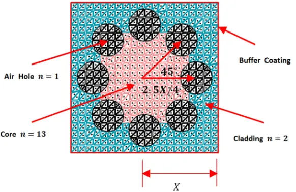
Figure 1 schematically represents the cross-section of HAPCF. The relative refraction coefficient of the core is assumed to be 13. The relative refraction coefficients of the cladding including the air holes surrounding the core symmetrically are 2 and 1, respectively. The central angle between neighboring air holes is made to be
4
⁄ radian. They are positioned symmetrically around the core, and the distance from the center of the fiber is 2.5 4⁄ , where arb. is a length from the center to the edge of the square HAPCF. In the course of FEM calculation, the space of cross section is divided into a mesh of triangular elements, as can be seen in figure 1. The total number of triangular elements, edges and nodes for the TM mode are 800,1240 and 441, respectively. The total number of triangular elements, edges and nodes for the TE mode are 800,1160 and 361, respectively. The number of differences for these TE and TM modes depends on the boundary conditions applied to the buffer coating.
Figure 1. Square HAPCF structure.
The eigenmodes are composed with the transverse vector fields and the longitudinal scalar fields. The transverse vector fields are represented by the edge vectors of the mesh elements. The longitudinal scalar fields are described with the nodes of the mesh elements. These eigenmode components are obtained simultaneously from the solution of the matrix eigen equation. The dimension of the matrix eigen equation is edge number node number , which is too large for a personal computer to perform. So, a sophisticated method such as the Krylov-Schur iteration method is carried out to obtain the several prominent eigenmodes. This method is described in the “Krylov-Schur iteration method” section.
The transverse vector field components thus obtained are schematically represented at the centroidal position of each triangular element. The longitudinal scalar modes are described in three dimensional shapes by the connecting the potential values at each node. And the contour lines of longitudinal scalar fields are obtained by projecting longitudinal spectra on the cross section of HAPCF.
2.2. Finite Element Method
procedures are applied for the electric field and magnetic field , except on the boundary condition. For the perfect conductor coating on the buffer layer of HAPCF, the Neumann and Dirichlet boundary condition are applied for TE and TM modes respectively. In this study, the calculation is focused on the procedure for field.
For convenience of discussion, it is assumed that the cross section and the axis of HAPCF are the xy plane and
z direction of the Cartesian coordinate, respectively. The vector Helmholtz wave equation for the electric field is given [7]
" # $&%'" # ( )*+, 0 (1)
where
. /01 231 45̂789:;4 (2)
and where <, and +, are the relative permeability and the relative permittivity, respectively. By separating the transverse vector fields and the z-directional longitudinal scalar fields, equation (1) can be described as
"=# "=# = &%'.> "= 4 > =7 )*+, = (3) %
&'?"=∙ ."= 4 > =7A )*+, 4 (4)
where
= /01 231 (5)
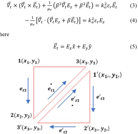
Figure 2. Orientational relations of edges of two adjacent triangular elements. For directional consistency, the edges of adjacent triangular elements must be in the same array as the first one. Therefore, the nodes of adjacent triangle elements should be arranged opposite to each other.
To make these equations suitable for numerical solutions, they are converted into weak forms. These forms are obtained by multiplying vector testing function B= to equation (3) and scalar testing function BC to equation (4), and performing the integrals on these equations in the triangular element area.
∬ B∆ =∙ .E=# E=# =7FG &%'∬ B∆ =∙ .> "= 4 > =7FG )*+,∬ B∆ =∙ =FG (6)
%
&'∬ B∆ C?"=∙ ."= 4 > =7AFG )*+,∬ B∆ C 4FG (7)
To perform the integration, it is necessary to use the Green’s theorem to reduce the order of derivatives [8]. The order of the triple product and the Laplacian operator can be reduced by using the first theorem of Greens formulae as follows
∬ B∆ =∙ ."=# "=# =7FG ∬ ."∆ =# B=7 ∙ ."=# =7FG I BK∆ =∙ ."=# =7 ∙ 1 FJ (8) ∬ B∆ C" 4FG I BK∆ C" 4∙ 1 FJ ∬ "B∆ C∙ " 4FG (9)
where 1 is the outward normal of the closed surface. On a perfect electric conducting boundary, the contour integral of equation (8) vanishes as B= is set to zero to satisfy the Dirichlet boundary conditions. And the contour integral on the right-hand side of equation (9) vanishes as BC is set to zero for the TM case and L 4⁄L vanishes for the TE case to satisfy the Neumann boundary condition. When the vector Helmholtz equation is divided into two equations, one equation is described by a tangential edge vector and the other by the node component of the triangular element. Then the transverse electric field is approximately given by the edge-based tangential vector, as follows
= ∑PNQ%8=NO=N (10)
where O=Nis the edge R vector of the triangular element. Its components are given with a simplex coordinate ST such as
O=% U=%.SPE=S S E=SP7 (11) O= U= .S%E=SP SPE=S%7 (12)
O=P U=P S E=S% S%E=S (13)
where U=T is a length of the tangential edge connecting the nodal points V and ). The z-direction longitudinal scalar field is described by the nodal based first order Lagrangian interpolation functions as
4 ∑ 8PTQ% 4TST (14)
where ST is the simplex coordinate of node W. The simplex coordinates are given with nodal points of the triangular element of figure 2.
XSS% SP
Y Z01 1 1% 0 0P
3% 3 3P
[ 9%
X10
3Y (15)
The tangential edge vectors of a triangular element are defined as shown in figure 2. For directional consistency, the edges of adjacent triangular elements must be in the same array as the first one. Applying Galerkin’s technique, the testing functions are the edge vector \=N and the simplex node function ST of the mesh element for equations (8) and (9), respectively.
equation
]^^_` == ^_` =4 _` 4= ^_` 44a $
8= 84( ]
B_` == 0
0 B_` 44 a $
8=
84( (16)
where each component of the square matrix is represented as
^_` == &%'∬ ."∆ =# O=N7 ∙ ."=# O=b7FG ; c
&'∬ .O∆ =N∙
O=b7 FG (17)
^_` =4 ;
c
&'∬ .O∆ =N∙ "=S:7FG (18)
^_` 4= ;
c
&'∬ ."∆ =S:∙ O=N7FG (19)
^_` 44 ;
c
&'∬ "S∆ T∙ "S: FG (20)
B_` == +,∬ .O∆ =N∙ O=b7FG (21)
B_` 44 +,> ∬ S∆ T∙ S:FG (22)
The global eigen equation results from combining these element matrices for total meshes.
d^ef8=*=g )*dBeh8i`*jk (23)
As a result, the eigenmodes are obtained by similarly transforming the matrix eigen equation into the Schur matrix. The column vectors of the similarity transformation matrix are the eigenmodes and the diagonal components of the Schur matrix are eigenvalues.
2.3. Krylov-Schur Iteration Method
In general, the dimensionality of the matrix eigen equation is very large. A personal computer cannot perform the calculation, especially for the inverse matrix of large dimensionality, in an ordinary manner. Therefore, a sophisticated method such as the Krylov-Schur iteration method is applied to overcome the problems [9]. It is well known that this method gives several prominent eigenmodes for the communicating optical fiber in robust way. This iteration method has previously been applied to various optical fibers and revealed their eigen properties of propagating waves [10]. To apply this iteration method, the global eigen equation is first converted to a shift invert form, like
%
lmc9n h8i`*jk dpe9ndoeo h8i`*jk dqeh8i`*jk (24)
The Krylov-Schur iteration method is applied to the matrix
dqe. By doing so, this strategy may be more efficiently implemented in finding specific eigen pairs at σ value. It can be summarized as follows:
[Krylov-Schur iteration method]
Input: Matrix dqe and assumed initial vector f8Tg with the number of the decomposition dimension, R.
Output: J s R Ritz pairs.
1. Build a Hessenberg matrix of order R by Arnoldi
decomposition [11].
2. Apply a QR algorithm to get a Schur matrix [12]. 3. Find the eigen pairs by the inverse iteration method. 4. If there are \ eigen pairs satisfying the pre-determined condition, reorder them to first primary diagonal block through the unitary similarity transform [13].
5. If J s \, truncate the result Schur matrix at position \. 6. Extend the matrix with the residual vector 8̃ 8̃uv%as an initial vector and go to step 1.
Similar to the previous study, the eigenmodes of the square HAPCF waveguide were obtained through the above procedure. The eigenmodes are the column vectors of the similarity transform matrix, which make matrix dqe into the Schur form. The eigenvector is separated into two components that describe the transverse vector field and the z-direction longitudinal scalar field. The transverse eigenmodes are described by the first w_ components of the column matrix. The remaining wb elements represent the z-direction longitudinal eigenmodes. The characteristics of the transverse vector eigenmodes at the center xy
0̅=,T, 3|=,T of the triangular element are obtained by applying equation (10) for each mesh element. The z-direction longitudinal eigenmodes of the triangular element are calculated from equation (14). The magnitude of each transverse vector y and y is normalized based on the maximum value of propagating modes. The magnitude of the z-direction longitudinal field is also normalized from the maximum value of the longitudinal scalar mode at each nodal point.
3. Results and Discussion
The Krylov-Schur iteration method was applied to the matrix dqe of equation (24) to obtain the eigenmodes of HAPCF. We have previously studied similar optical fiber systems. The study [5] was about a square PCF that was not the same as this study. The square PCF consisted of a core and holes without the cladding. The eigenmodes did not include the contour lines of the longitudinal eigenmodes on the cross section of the fiber. The study in reference [6] was for circular HAPCF. It was constructed similar to conventional fiber, including holes at the interface between the core and the cladding. The resulting eigenmodes were schematically represented with the transverse vector fields, the longitudinal scalar fields represented in the three dimensional space and their contours lines projected onto the xy-plane of the fiber. But there were no TM eigenmodes that combined with TE modes to illustrate the eigen property of circular HAPCF more developmentally. So, some additional information related to the longitudinal scalar field of TE and TM modes is needed for a better understanding of the eigen property of HAPCF.
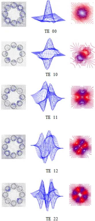
Figure 4. TE eigenmodes of HAPCF. In contrast to the TM mode, there is a distribution of the transverse electric field in the cladding and air holes. The equipotential contours, combined with the three-dimensional representation of electric scalar potential, give indispensable information to determine the mode type of the spectra.
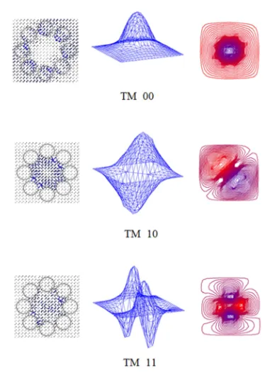
In this study, a square HAPCF similar to a circular HAPCF was constructed. There are more mesh elements because of expanding the space of cross-section from the circular to square forms of HAPCF. But the density of the mesh element is not different from the circular one. As mentioned in figure 1, the buffering layer is assumed to be coated with the perfect conductor for TM modes. This boundary condition differentiates the FEM calculation between TM and TE modes. When calculating the TM mode, the node and edge components on the buffer coating surface are ignored by the Dirichlet and Neumann boundary condition, respectively. The results of the calculation for TM eigenmodes are illustrated in figure 3. As can be seen in the first column of this figure, the transverse magnetic field is confined to the core region. The conventional fiber consisting only of a core and cladding permit leakage over the interface between them. For PCF made with the core and multiple air holes without dielectric cladding, leakage can not be excluded over the core. But the buffer of HAPCF coated with a perfect conductor confines the propagating wave to the core and permits only small leakage over the interface. From this result, it can be said that the wave sees the prominent refractive difference between the effective cladding and the core. The refractive index of effective cladding is composed of contributions from the cladding, air holes and the buffer of the perfect conductor. The exact index difference between the core and the effective cladding cannot be determined from conventional theory, but only estimated experimentally. The second column of figure 3 reveals the z-direction longitudinal magnetic field. Together with the relation of the transverse magnetic vector field, the mode types are determined and notified as shown under each spectrum. The longitudinal scalar fields more clearly represent the eigen properties of HAPCF. Comparing the transverse spectra, the peak intensity of the longitudinal field is higher at the position where the magnetic field is strong. The determination for the mode type is more clear by investigating the contour lines of the longitudinal fields, as shown in the third column of figure 3. These spectra are obtained by projecting the spectra of the second column onto the cross section of HAPCF (or xy-plan of Cartesian coordinate). In these spectra, peak positions and their intensity are clear, and represented by color intensity. Contour lines are continuously distributed, do not cross each other and do not terminate at the surface. These are reasoned from the boundary condition that excludes the magnetic field and z-direction longitudinal scalar field from the surface. In other words, it can be conjectured that the boundary condition from the buffer surface of the perfect conductor contributes to clearly identify the eigenmode with FEM numerical calculation.
continuously across the cross section of HAPCF, but terminated at the buffer layer. This appearance of spectra is prominently different from the TM modes. It is difficult to classify the mode type of spectra into TM and TE by transverse vector field or scalar potential. In particular, the transverse field is not sufficient for determining the mode type of HAPCF because the transverse field is shielded by the air holes and their strength is weakened at the buffer layer. So, the mode type can be clearly determined by investigating the contour lines of the longitudinal scalar fields in addition to the transverse field vectors.
The interpretation for the transverse field of the TE spectra is not as simple as the MT mode. The electric field is not completely constrained to the core area. The components of this field extend beyond the air holes to the cladding region. This is in contrast to the TM mode, where the transverse field is completely restricted to the core region. This phenomenon can be presumed to be caused by the different boundary conditions applied to the two systems. For the TM mode, it was assumed that the buffer layer is coated with the perfect conductor. With the Dirichlet boundary condition, it can be said that the field components are excluded from the conductor coating layer. Due to this effect, it can be understood that the formation of the TM mode is restricted to the core area. In the case of the TE mode, only the cladding and the air holes function to shield the transverse wave. It has previously been shown that the effect of shielding the transverse waves depends on the changes of position of air holes and their numbers. The results meant that in order to effectively shield the transverse waves, many air holes must be arranged in a multiple structure [14]. And air holes with a low refractive index should limit the spatial distribution of the transverse waves and concentrate them in the core area. For the TM mode, this function is performed by the buffer layer coated with a perfect conductor.
The third column in figure 4. plays an important role in determining the mode type, as in the TM mode.The spectra of several prominent eigenmodes are schematically represented in the figure along with the mode type. The peak position and intensity of these spectra are represent the characteristics of mode type. Unlike in previous studies, the contour lines of the longitudinal electric field contribute a lot of to determining the mode type. In other words, these spectra contribute to determining a definite mode type together with their three-dimensional representation.
4. Conclusion
FEM has been carried out to investigate the eigenmodes constructed in square HAPCF. The spectra of TM and TE modes were plotted with the transverse vector field, longitudinal scalar fields and their contour lines onto the cross section of the HAPCF. The mode types were mainly determined by the contour lines of the longitudinal scalar
fields together with their three dimensional representation. Comparing the spectra of TM and TE modes, it was identified that the buffer coated with a perfect conductor functioned importantly in constructing the eigenmodes for HAPCF.
References
[1] Russel Philip St. John, “Photonic Crystal Fibers,” Science, Vol 299, No. 5605 pp 358-362, 2003.
[2] Jan Sporik, Miloslave Filka, Vladimir Tejkal, Pavel Reichert, “Principle of photonic crystal fibers,” Elektroevue, Vol. 2, No. 2, June 2011.
[3] JC Knight, TA Birks, P. St. J. Russell, Dale Atkin “All-silica single-mode optical fiber with photonic crystal cladding: Errata,” Optics Letters 22(7), 484-7, May 1997.
[4] X. Yu, P. Shum, M. Yan, J. Love “Numerical investigations of interstitial hole-assistant microstructured optical fiber,” Journal of Optical Electronics and Advanced Materials Vol. 8, No. 1, pp. 372-375, Feb. 2006.
[5] Yeong Min Kim “A study on the eigenmodes of a square PCF depending on wave numbers,” IEIE Transactions on Smart Processing & Computing Vol. 6, No. 5, 365-371, Oct. 2017. [6] Yeong Min Kim, Se Jung Oh “A study on the Eigenmodes
Constructed in the HAPCF,” HSST, Vol. 8, No. 11, pp. 223-233, Nov. 2018.
[7] C. J. Reddy, Manohar D. Deshpande, C. R. Cockrell, and Fred B. Beck, “Finite Element Method for Eigenvalue Problems in Electromagnetics,” NASA Technical Paper 3485, Dec. 1994. [8] Peter P. Silvester and Ronald L. Ferrari, “Finite elements for
Electrical Engineers 3rd ed.,” Cambridge University Press, App. 2, pp. 459-463, 1996.
[9] G. W. Stewart, “A Krylov Schur Algorithm for Large Eigenproblems” SIAM J. Matrix Anal. & Appl. Vol. 23, No. 3, pp. 601-614, 2002.
[10] Yeong Min Kim “A Study on the Eigen Modes of PCF Varying the Position of the Dielectric Holes by FEM,” Global Journal of Engineering Science and Researches, Vol. 3, No. 7, pp. 130-135, July 2016.
[11] V. Hernandez, J. E. Roman, A. Tomas, V. Vidal, “Arnoldi Methods in SLEPc,” SLEPc Technical Report STR-4 Available at http://www.grycap.upv.es/slepc
[12] David S. Watkins, “The QR Algorithm Revisited,” SIAM Review, Vol. 50, No. 1, pp. 133–145, Feb. 2008.
[13] Maysum Panju “Iterative Methods for Computing Eigenvalues and Eigenvectors” University of Waterloo, http://mathreview.uwaterloo.ca