Bayesian Graphical Models for Multivariate Functional Data
Hongxiao Zhu [email protected]
Department of Statistics
Virginia Tech, 250 Drillfield Drive (MC 0439) Blacksburg, VA 24061, USA
Nate Strawn [email protected]
Department of Mathematics and Statistics Georgetown University
Washington D.C. 20057, USA
David B. Dunson [email protected]
Department of Statistical Science Duke University
Durham NC 27708, USA
Editor:Jie Peng
Abstract
Graphical models express conditional independence relationships among variables. Al-though methods for vector-valued data are well established, functional data graphical mod-els remain underdeveloped. By functional data, we refer to data that are realizations of random functions varying over a continuum (e.g., images, signals). We introduce a notion of conditional independence between random functions, and construct a framework for Bayesian inference of undirected, decomposable graphs in the multivariate functional data context. This framework is based on extending Markov distributions and hyper Markov laws from random variables to random processes, providing a principled alternative to naive application of multivariate methods to discretized functional data. Markov properties facil-itate the composition of likelihoods and priors according to the decomposition of a graph. Our focus is on Gaussian process graphical models using orthogonal basis expansions. We propose a hyper-inverse-Wishart-process prior for the covariance kernels of the infinite co-efficient sequences of the basis expansion, and establish its existence and uniqueness. We also prove the strong hyper Markov property and the conjugacy of this prior under a finite rank condition of the prior kernel parameter. Stochastic search Markov chain Monte Carlo algorithms are developed for posterior inference, assessed through simulations, and applied to a study of brain activity and alcoholism.
Keywords: graphical model, functional data analysis, gaussian process, model uncer-tainty, stochastic search
1. Introduction
hyper-Markov laws serving as prior distributions in Bayesian analysis. The special case of Gaussian graphical models, in which a multivariate Gaussian distribution is assumed and the graph structure corresponds to the zero pattern of the precision matrix (Dempster, 1972; Lauritzen, 1996), is well studied. Computational algorithms, such as Markov chain Monte Carlo (MCMC) and stochastic search, are developed to estimate the graph based on the conjugate hyper-inverse-Wishart prior and its extensions (Giudici and Green, 1999; Roverato, 2002; Jones et al., 2005; Scott and Carvalho, 2008; Carvalho and Scott, 2009).
In the frequentist literature, notable works on graphical models include the graphical LASSO (Yuan and Lin, 2007; Friedman et al., 2008; Mazumder and Hastie, 2012a,b) and the neighborhood selection approach (Meinshausen and B¨uhlmann, 2006; Ravikumar et al., 2010). The graphical LASSO induces sparse estimation of the precision matrix of the Gaussian likelihood through l1 regularization. The neighborhood selection approach relies
on estimating the neighborhood of each node separately by regressing each variable on all the remaining variables, sparsifying withl1regularization, and then stitching the neighborhoods
together to form the global graph estimate. Various extensions, computational methods, and theoretical properties have been developed in these frameworks (Lam and Fan, 2009; H¨ofling and Tibshirani, 2009; Cai et al., 2011; Witten et al., 2011; Yang et al., 2012; Mazumder and Hastie, 2012a,b; Anandkumar et al., 2012; Loh and Wainwright, 2013).
The graphical modeling literature focuses primarily on vector-valued data with each node corresponding to one variable. Many applications, however, involvefunctional data— data that are realizations of random functions varying over a continuum such as a time interval or a spatial domain. Common types of functional data include signals, images, and many emerging high-throughput digital measurements. The dependence structure of functional data is of interest in a wide range of applications. For example, in neuroimaging, we are often interested in the dependence network across brain regions, where data from each region are of functional form (e.g., EEG/ERP signals, MRI/fMRI regions). In bioin-formatics, we often need to model gene networks based on time-course gene expression data (Ma et al., 2006), treating each time-course as a continuous process. In epigenetics, it is of interest to study how cells are differentiated into organs (cell lineage and differentiation) by exploring the dependence structure of genome-wide methylation levels across different cell types, and for each cell type, the methylation level can be considered as a function of the genomic locations.
func-tions. Through representing the random functions with orthogonal basis expansions, we transform functional data from the function space to the isometrically isomorphic space of basis coefficients, where Markov distributions and hyper Markov laws can be conveniently constructed. We further propose a hyper-inverse-Wishart-process prior for the covariance kernels of the coefficient sequences, and study theoretical properties of the proposed prior such as existence and uniqueness. We also establish the strong hyper Markov property and conjugacy of this prior under a finite rank condition for the prior kernel parameter, which implies that the covariance kernel of the coefficient sequences is a priori finite dimensional. To perform posterior inference, we introduce a regularity condition which allows us to write the likelihood and prior density and design stochastic search MCMC algorithms for poste-rior sampling. Performance of the proposed approach is demonstrated through simulation studies and analysis of brain activity and alcoholism data.
To our knowledge, the proposed approach is the first considering functional data graph-ical models from a Bayesian perspective. It extends the theory of Dawid and Lauritzen (1993) from multivariate data to multivariate functional data. Most existing graphical model approaches often naively apply multivariate methods to functional data after per-forming discretization or feature extraction. Such approaches may not take full advantage of the fact that data arise from a function and can lack reasonable limiting behavior. Our graphical model framework guarantees proper theoretical behavior as well as computational convenience.
2. Graphical Models for Multivariate Functional Data
In this section, we first review graphical models for multivariate data in Section 2.1, then introduce graphical models for multivariate functional data in Section 2.2, and finally present the specific case of Gaussian process graphical models in Section 2.3.
2.1 Review of Graph Theory and Gaussian Graphical Models
We follow Dawid and Lauritzen (1993), Lauritzen (1996), and Jones et al. (2005). Let G = (V, E) denote an undirected graph with a vertex set V and a set of edge pairs E =
{(i, j)}. Each vertex corresponds to one variable. Two variables aand b are conditionally independent if and only if (a, b) ∈/ E. A graph or a subgraph is complete if all possible pairs of vertices are joined by edges. A complete subgraph ismaximal if it is not contained within another complete subgraph. A maximal subgraph is called a clique. If A, B, C are subsets of V with V = A∪B, C = A∩B, then C is said to separate A from B if every path from a vertex in A to a vertex in B goes through C. C is called a separator
and the pair (A, B) forms a decomposition of G. The separator is minimal if it does not contain a proper subgraph which also separates A from B. While keeping the separators minimal, we can iteratively decompose a graph into a sequence of prime components – a sequentially defined collection of subgraphs that cannot be further decomposed (Jones et al., 2005). If all the prime components of a connected graph are complete, the graph is called
decomposable. All the prime components of a decomposable graph are cliques. Iteratively decomposing a decomposable graph Gproduces aperfectly orderedsequence of cliques and separators (C1, S2, C2, . . . , Sm, Cm) such thatSi =Hi−1∩Ci and Hi−1 =C1∪ · · · ∪Ci−1.
separators. The perfect ordering means that for every i= 2, . . . , m, there is a j < i with Si ⊂Cj (Lauritzen, 1996, page 15).
If the components of a random vectorX= (X1, . . . , Xp)T obey conditional independence
according to a decomposable graph G, the joint density can be factorized as
p(X|G) = Q
C∈Cp(XC)
Q
S∈Sp(XS)
,
whereXA={Xi, i∈A}. IfX is Gaussian with zero mean and precision matrixΩ=Σ−1,
thenXi is conditionally independent ofXj given XV\{i,j}, denoted by Xi ⊥⊥Xj |XV\{i,j},
if and only if the (i, j)th element of Ωis zero. In this casep(X|G) is uniquely determined by marginal covariances {ΣC,ΣS, C ∈ C, S ∈ S}, which are sub-diagonal blocks of Σ
according to the clique and separator sets. For a given G, a convenient conjugate prior for
Σis hyper-inverse-Wishart (HIW) with density
p(Σ|G, δ,U) = Q
C∈Cp(ΣC |δ,UC)
Q
S∈Sp(ΣS |δ,US)
,
wherep(ΣC |δ,UC) andp(ΣS|δ,US) are densities of inverse-Wishart (IW) distributions. In this paper, the inverse-Wishart follows the parameterization of Dawid (1981), i.e., Σ∼
IW(δ,U) if and only ifΣ−1 has a Wishart distribution W(δ+p−1,U−1), whereδ >0 and
Σis ap by pmatrix.
2.2 Graphical Models for Multivariate Functional Data
Let f = {fj}pj=1 denote a collection of random processes where each component fj is
in L2(Tj) and each Tj is a closed subset of the real line. The domain of f is denoted by
T =Fp
j=1Tj, whereFdenotes the disjoint union defined byFpj=1Tj =Spj=1{(t, j) :t∈Tj}.
For each j, let {φjk}∞k=1 denote an orthonormal basis of L2(Tj). The extended basis
functions ψjk = (0, . . . ,0, φjk,0, . . . ,0), with φjk in the jth component and 0 functions
elsewhere for j = 1, . . . , p and k = 1, . . . ,∞, form an orthonormal basis of L2(T). Let (L2(T),B(L2(T)), P) be a probability space, where B(L2(T)) is the Borel σ-algebra on
L2(T). For V = {1,2, . . . , p} and A ⊂ V, denote by fA the subset of f with domain TA =Fj∈ATj. We define the conditional independence relationships for components of f
in Definition 1.
Definition 1 Let A, B, and C be subsets of V. Then fA is conditionally independent of fB given fC under P, written as fA ⊥⊥ fB | fC[P], if for any fA ∈ DA, where DA is a measurable set in L2(T
A), there exists a version of the conditional probability P(fA∈DA| fB,fC) which is B(L2(TC)) measurable, and hence one may write P(fA∈ DA |fB,fC) =
P(fA∈DA |fC). Here,B(L2(TC))denotes the Borel σ-algebra on L2(TC). Note that this implies P(fA∈DA,fB∈DB |fC) =P(fA∈DA|fC)P(fB ∈DB|fC).
Definition 2 Let G= (V, E)denote a decomposable graph. A probability measure P off is called Markov over G if for any decomposition(A, B) of G, fA⊥⊥fB |fA∩B[P].
Given a decomposable graph G, a probability measure of f with Markov property may be constructed. To enable the construction, we first state Lemma 1, which generalizes Lemma 2.5 of Dawid and Lauritzen (1993) from the random variable to the random process case.
Lemma 1 Let f = (f1, . . . , fp) be a collection of random processes in L2(T). For subsets
A, B ⊂V = {1, . . . , p} with A∩B 6= ∅, suppose that P1 and P2 are probability measures of fA andfB, respectively. If P1 and P2 are consistent, meaning that they induce the same measure for fA∩B, then there exists a unique probability measure P for fA∪B such that (i)
PA= P1, (ii) PB =P2, and (iii) fA ⊥⊥fB |fA∩B[P]. The measure P is called a Markov combination of P1 and P2, denoted as P =P1?P2.
We provide a proof of Lemma 1 through construction in Appendix B. The main idea is to first construct the conditional probability P1{· |πA∩B(fA)} from P1, where πA∩B :
L2(T
A) →L2(TA∩B) is a projection map andTA=Fj∈ATj. We then defineP{ · |πB(f)}
based upon P1{· |πA∩B(fA)} using disintegration theory (Chang and Pollard, 1997), and
finally construct the joint measure P that satisfies conditions (i)–(iii). With Lemma 1, we can construct a joint probability measure for f that is Markov over G. The construction is based on the perfectly ordered decomposition (C1, S2, C2, . . . , Sm, Cm) of G with Si =
Hi−1∩Ci and Hi−1 =C1∪ · · · ∪Ci−1. Let {MCi, i = 1, . . . , m} be a sequence of pairwise
consistent probability measures for{fCi, i= 1, . . . , m}. We construct a Markov probability
measure P overGthrough the following recursive procedure
PC1 = MC1, (1)
PHi+1 = PHi?MCi+1, i= 1, . . . , m−1. (2)
One can show that the probability measure constructed this way is the unique Markov probability measure overG with marginals {MCi}, and the proof follows that of Theorem
2.6 in Dawid and Lauritzen (1993). We call the probability distribution induced by the probability measure constructed above theMarkov distribution off overG.
Denote the Markov distribution of f constructed in (1) - (2) by PG, and denote the
space of all Markov distributions over G by M(G). A prior law forPG is then supported
on M(G). We follow Dawid and Lauritzen (1993) to define hyper Markov laws and use them as prior laws for PG. A prior law L of PG is called hyper Markov over G if for any
decomposition (A, B) of G, (PG)A ⊥⊥ (PG)B | (PG)A∩B[L], where (PG)A takes values in
M(GA) which is the space of all Markov distributions over subgraph GA. Here, we have
assumed that G is collapsible onto A, therefore φ ∈ M(GA) if and only if φ= (PG)A for
some (PG) ∈ M(G). The following Proposition 1 states that the theory of hyper Markov
laws of Dawid and Lauritzen (1993) applies to our random process setup.
Proposition 1 The theory of hyper Markov laws over undirected decomposable graphs, as described in Section 3 of Dawid and Lauritzen (1993), holds for random processes.
According to the theory of hyper Markov laws, one can construct a prior law for PG
Denote byLG the constructed hyper Markov prior forPG and by Π a prior distribution for
the graphG. A Bayesian graphical model for the collection of random processes f can be described as
f ∼PG; PG∼LG; G∼Π. (3)
As we have yet to specify a concrete example for the probability measure PG, the above
Bayesian framework remains abstract at the moment. In Section 2.3, we construct PG
using Gaussian processes and propose a hyper-inverse-Wishart-process law as the prior for PG. The prior distribution Π is supported on the finite dimensional space of decomposable
graphs withp nodes.
2.3 Gaussian Process Graphical Models for Multivariate Functional Data
Let f0 = (f01, . . . , f0p) be an element in L2(T). Denote by K = {kij : Ti×Tj → R}
a collection of covariance kernels such that cov{fi(s), fj(t)} = kij(s, t), s∈ Ti, t∈ Tj. We
assume thatK is positive semidefinite and trace class. Positive semidefinite means that
p
X
i,j=1 ∞
X
k,l=1
cikcjl
Z
Tj
Z
Ti
kij(s, t)φik(s)φjl(t)dsdt≥0
for any square summable sequence{cik, i= 1, . . . , p, k= 1, . . . ,∞}; trace class means that
p
X
j=1 ∞
X
l=1
Z
Tj
Z
Ti
kjj(s, t)φjl(s)φjl(t)dsdt <∞.
Then f0 and K uniquely determine a Gaussian process on L2(T) (Prato, 2006), which we
call a multivariate Gaussian process, and writeMGP(f0,K). The definition of multivariate
Gaussian process implies that for A ⊂V,fA∼MGP(f0A,KA) where KA ={kij, i, j ∈A}.
Furthermore, on a sequence of cliques C = {C1, . . . , Cm}, the marginal Gaussian process
measures for {fC, C ∈ C} are automatically consistent because they are induced from the same joint distribution. Therefore, we can construct a Markov distribution for f over G through procedure (1) - (2). We denote the resulting distribution of f by MGPG(f0,KC),
where KC ={kij :i, j ∈C, C ∈ C}. It is clear from this construction that the distribution MGPG is Markov overGwhereas MGPis not.
For the convenience of both theoretical analysis and computation, we represent ele-ments in L2(T) using orthonormal basis expansions and construct a Bayesian graphical model in the dual space of basis coefficients. Let {φjk}∞k=1 denote an orthonormal
ba-sis of L2(Tj). For example, {φjk}∞k=1 could be a wavelet basis. We have the
represen-tation fj(t) = P∞k=1cjkφjk(t) where cjk = hfj, φjki =
R
Tjfj(t)φjk(t)dt. The coefficient
sequence cj ={cjk, k= 1, . . . ,∞}lies in the space of square-summable sequences, denoted
by`2j = n
cjk :P∞k=1c2jk <∞
o
. Denote`2=Qp
j=1`2j. Since`2j and L2(Tj) are isometrically
the coefficient sequence off. Thenf ∼MGP(f0,K) corresponds toc∼dMGP(c0,Q), where dMGP denotes the infinite dimensional discrete multivariate Gaussian processes, c0 is the coefficient sequence of f0 and Q={qij(·,·), i, j ∈V}. Here, qij is the covariance kernel so
that cov(cik, cjl) =qij(k, l) for k, l∈ {1,2,3, . . .}. Similarly, f ∼MGPG(f0,KC) corresponds
to c ∼ dMGPG(c0,QC) where QC = {qij(·,·), i, j ∈ C, C ∈ C}. The collection Q is also
positive semidefinite and trace class, so thatPp
i,j=1
P∞
k,l=1cikcjlqij(k, l)≥0 for any square
summable sequence {cik, i = 1, . . . , p, k = 1, . . . ,∞}, and Ppj=1
P∞
k=1qjj(k, k) < ∞.
Fur-thermore, K relates to Q through equation kij(s, t) = P∞k,l=1qij(k, l)φik(s)φjl(t). Denote
by Pc and Pf the probability measures of c and f respectively, then fA ⊥⊥ fB | fC[Pf]
implies cA ⊥⊥ cB | cC[Pc] and vice versa. Thus, the distribution dMGPG(c0,QC) of c is
again Markov.
Assume thatc∼dMGPG(c0,QC). The parameters involved in this distribution include c0 and QC. In this study, we assume that c0 is fixed (e.g., a zero sequence) so that the
distribution ofc is uniquely determined by QC. As indicated in Section 2.2, we would like
to construct a hyper Markov law for the dMGPG distribution. Since dMGPG is uniquely determined byQC, it is equivalent to construct a hyper Markov law forQC. Given a positive
integer δ and a collection U = {uij : N×N → R, i, j ∈ V} which is symmetric, positive
semidefinite, and trace class, we construct a hyper-inverse-Wishart-process (HIWP) prior forQC following Theorem 1.
Theorem 1 Assume that c∼dMGPG(c0,QC). Suppose thatδ is a positive integer, and
U is a collection of kernels that is symmetric, positive semidefinite and trace class. Then there exists a sequence of pairwise consistent inverse-Wishart processes determined by δ and UC ={uij, i, j ∈C}, C ∈ C, based on which one can construct a unique hyper Markov
law for QC, which we call a hyper-inverse-Wishart-process, and write QC ∼HIWPG(δ,UC),
whereUC={uij, i, j∈C, C∈ C}.
Based on Theorem 1, a Bayesian Gaussian process graphical model can be written as
c∼dMGPG(c0,QC), QC∼HIWPG(δ,UC), G∼Π. (4)
It is of interest to investigate the properties of the HIWP prior and the corresponding posterior distribution. As shown in Dawid and Lauritzen (1993), one nice property of the HIW law is the strong hyper Markov property, which leads to conjugacy as well as convenient posterior computation at each clique. In case of the HIWP prior, the strong hyper Markov property is defined such that for any decomposition (A, B) ofGin model (4),QB|A⊥⊥ QA,
where QB|A denotes the conditional distribution (i.e., conditional covariance) of cB given cA. In the following proposition, we show that theHIWPG prior constructed in Theorem 1
is strong hyper Markov when rank(uij)<∞ fori, j∈V.
Proposition 2 Suppose that the collection of kernels U satisfies that rank(uij) <∞ for
i, j∈V, then the hyper-inverse-Wishart-process prior constructed in Theorem 1 satisfies the strong hyper Markov property. That is, if QC∼HIWPG(δ,UC), then for any decomposition
(A, B)ofG,QB|A⊥⊥ QA, whereQB|Adenotes the conditional distribution (e.g., conditional covariance) ofcB givencA.
The finite rank condition for the prior parameters {uij} in Proposition 2 is a relatively
implies that the covariance kernel QC, thus the sequence c, is a priori finite dimensional.
Whether the strong hyper Markov property still holds without this condition remains a challenging open problem. In the online appendix, we have included several interesting results made through our preliminary study, which may provide useful insights into further investigations of this problem. The strong hyper Markov property of HIWPG ensures that
the joint posterior ofQC (conditional onG) can be constructed from the marginal posterior
of QC (conditional on G) at each clique C, as stated in Theorem 2. Therefore one essen-tially transforms the Bayesian analysis to a sequence of sub-analyses at the cliques, which substantially reduces the size of the problem.
Theorem 2 Suppose that ci ∼dMGPG(c0,QC), i= 1, . . . , n are independent and
identi-cally distributed. Further assume that the prior of QC isHIWPG(δ,UC) where the collection
of kernels U satisfies that rank(uij) < ∞ for i, j ∈ V. Then the conditional posterior of
QC given {ci} and G is HIWPG(eδ,UeC), where δe= δ+n, UeC = {ueij, i, j ∈ C, C ∈ C} and
e
uij = uij +Pni=1(ci −c0i)⊗(cj −c0j). Here ⊗ denotes the outer product. Furthermore, the marginal distribution of {ci} given{G,c0, δ,UeC} is again Markov over G.
Theorem 2 implies that when rank(uij) < ∞ for i, j ∈ V, the HIWPG(δ,UC) prior is
a conjugate prior for QC in the dMGPG(c0,QC) likelihood. Note that here the likelihood,
the prior, and the posterior are all conditional on G, which makes Bayesian inference of G tractable. Model (4) and results in Theorem 2 provide the theoretical foundation for practical Bayesian inference under a reasonable regularity condition, as discussed in Section 3.
3. Bayesian Posterior Inference
Despite the fact that functional data are realizations of inherently infinite-dimensional random processes, data can only be collected at a finite number of measurement points. Essentially, estimating the conditional independence structure of infinite-dimensional ran-dom processes based on a finite number of measurement points is an inverse problem and therefore requires regularization. M¨uller and Yao (2008) reviewed two main approaches for regularization in functional data analysis—finite approximation through, e.g., suitably truncating the basis expansion representation and penalized likelihood. In this paper, we suggest performing posterior inference based on approximating the underlying random pro-cesses with orthogonal basis functions. In particular, we assume the following regularity condition:
Condition 1 The functional data f are observed discretely on a dense grid t = F
tj with tj = (tj1, . . . , tjmj(n)) and mj(n) → ∞ as n → ∞. One can find Mj(n) so that the underlying random process fj can be approximated with an Mj-term orthogonal basis expansion fbj =
PMj
l=1cjlφjl, with approximation error ||fj−fbj||L2 =Op(n−β) with β≥1/2 for all j∈V.
Essentially, Condition 1 requires that the discretely-measured functional data capture sufficient information about the underlying random processes, so that we can approximate each fj with a negligible approximation error. This condition provides the consistency of
whenMj increases with the sample sizen. We need such a condition in order to guarantee
that the behavior of{fj}is not too outrageous. Certain assumptions, such as the decay rate
of the eigenvalues of fj, the smoothness property of fj, or the characteristics of the basis
functions, will determine the specific rate β (De Boor, 2001; Jansen and Oonincx, 2015). However, under our generic setup, since we prefer not to specify particular assumptions, we only require a mild range for the convergence rate. Condition 1 is a basic assumption in the functional setting, and a similar regularity condition has been adopted by Qiao et al. (2015) in a functional graphical model based on the group LASSO penalty.
3.1 Bayesian Posterior Inference under the Regularization Condition
The regularity from Condition 1 enables us to write the density functions of the Markov distributions and hyper Markov laws so that posterior inference can be practically imple-mented. Denoting M = (M1, . . . , Mp), we can explicitly write the density function for the
truncated processcM = (cM1 1 , . . . , c
Mp
p ), and an MCMC algorithm can then be designed for
the posterior inference of the underlying graphG. The density function of cM is
p(cM |cM0 ,QC, G) = Q
C∈Cp(cMC |cM0,C,QC)
Q
S∈Sp(cMS |cM0,S,QS)
, (5)
whereQC is a block-wise covariance matrix with the (i, j)th block formed by{qij(k, l), k=
1, . . . , Mi, l = 1, . . . , Mj}, and QC, QS are submatrices of QC corresponding to clique C
and separator S, respectively. The HIWPG prior of QC induces a hyper inverse-Wishart
prior with density
p(QC |G) =
Q
C∈Cp(QC |δ,UC)
Q
S∈Sp(QS|δ,US)
, (6)
where p(QC | δ,UC) is the density of inverse-Wishart defined in Dawid (1981), UC is a
submatrix ofUC corresponding to cliqueC, andUC is a block-wise matrix formed by{uij}
in the same way asQCis formed by{qij}. Thep(QS|δ,US) component in the denominator
is defined similarly. Based on (5) and (6), and assuming that{ci, i= 1, . . . , n}is a random
sample ofc, one can further integrate outQC to get the marginal density
p({cMi } |cM0 , G) = (2π)−n2( P
iMi)h(δ,UC)
h(eδ,UeC)
, (7)
where
h(δ,UC) =
Q
C∈C|12UC|
(δ+dc−2 1)Γ−1 dc{
1
2(δ+dc−1)}
Q
S∈S|12 US|
(δ+ds−2 1)Γ−1
ds{12(δ+ds−1)}
,
anddcanddsare the dimensions ofUC andUSrespectively, and Γb(a) =πb(b−1)/4Qbi=0−1Γ(a−
i/2). The denominator h(δ,e UeC) in (7) is defined in the same way. Based on these results,
posterior inference can be done through sampling from the posterior density
where p(G) is the density function corresponding to the prior distribution G ∼ Π, which is a discrete distribution supported on all decomposable graphs with pnodes. Giudici and Green (1999) used the discrete uniform prior Pr(G = G0) = 1/d for any fixed p-node
decomposable graph G0, where d is the total number of such graphs; Jones et al. (2005)
used the independent Bernoulli prior with probability 2/(p−1) for each edge, which favors sparser graphs (Giudici, 1996). The following MCMC algorithm describes the steps to generate posterior samples based on (8).
Algorithm 1
Step 0. Set an initial decomposable graph Gand set the prior parameters c0,δ, and UC.
Step 1. With probability 1−q, propose Ge by randomly adding or deleting an edge from G
(each with probability 0.5) within the space of decomposable graphs; with probabil-ity q, propose Ge from a discrete uniform distribution supported on the set of all
decomposable graphs. Accept the new Ge with probability
α= min (
1,p(Ge| {c
M
i },cM0 ) p(G|G)e p(G| {cM
i },cM0 ) p(Ge|G) )
.
Repeat Step 1 for a large number of iterations until convergence is achieved.
Detailed derivations are available in the online appendix. The above algorithm is a Metropolis-Hastings sampler with a mixture of local and heavier-tailed proposals, also called a small-world sampler. The “local” move involves randomly adding or deleting one edge based on the current graph, and the “global” move is achieved through the discrete uniform proposal. Guan et al. (2006) and Guan and Krone (2007) have shown that the small-world sampler leads to much faster convergence especially when the posterior distribution is either multi-modal or spiky.
3.2 Bayesian Posterior Inference for Noisy Functional Data
The theory in Section 2 and the posterior inference in Section 3.1 relies on the assumption that the distribution off (andc) is Markov overG. In many situations, it is more desirable to make such an assumption in a hierarchical model. For example, when functional data are subject to measurement error, one might wish to incorporate an additive error term and consider the following model
yijt=fij(t) +εijt, i= 1, . . . , n, j = 1, . . . , p, t∈tj, (9)
where {yijt, t ∈ tj} are noisy observations measured on a dense grid tj = (tj1, . . . , tjmj),
{fij} are the underlying true functions, and {εijt, t ∈ tj} are measurement errors. We
assume that{fij} and {εijt, t∈tj} are mutually independent of each other. The inference
of model (9) involves both smoothing (i.e., estimatingfij) and estimation of the underlying
graph G. We achieve these goals simultaneously through fitting a Bayesian hierarchical model.
In particular, we assume that{fij}are Gaussian processes inL2(Tj), and denote{cijk}
their basis coefficients corresponding an orthonormal basis{φjk}∞k=1. With this
process. We further assume that the measurement error εij = {εijt, t ∈ tj} is Gaussian
white noise with variance σ2j, i.e., εijt ∼ N(0, σ2j) independently across all t for t ∈ tj.
Truncating at theMjth basis element, we can reparameterize the model as
yijt= Mj
X
k=1
cijkφjk(t) +εeijt, t∈tj (10)
whereεeijt is a new residual term that consists of the approximation error of the truncated
series (e.g., P∞
k=Mj+1cijkφjk(t)) and the measurement error. If we concatenate the noisy
observations to form a vector
yi = (yi1t11, . . . , yi1t1m1, . . . , yiptp1, . . . , yiptpmp) T
and denotecMi the vector formed by the basis coefficients{cijk, j= 1, . . . , p, k= 1, . . . , Mj},
then model (10) can be written as yi = ΦcMi +eεi, where Φ = diag{φ1, . . . ,φp} is a P
jmj by PjMj block-diagonal matrix with the jth diagonal block containing φj =
[φj1(tj), . . . , φjMj(tj)], andeεidenote the concatenated vector of the new residual terms. We assume thateεi∼N(0,Λ) whereΛ= diag(s
2
11Tm1, . . . , s 2
p1Tmp). Notice that ifQC= cov(cMi ),
then cov(yMi ) = ΦQCΦT +Λ. The diagonals of ΦQCΦT and Λ can not be separately
identifiable. Therefore, we treat Λ as a fixed model parameter, whose quantity can be pre-determined by the approximations2j ≈bσj2, whereσb2j is the estimation ofσj2 using local smoothing on{εijt}.
Applying a prior for cMi in the form of (5) (conditional on G) and theHIWPG prior for
the covariance matrix QC in the form of (6), we obtain the density function for the joint
posterior
p({cMi },QC, G| {yi})∝ n
Y
i=1
p(yi|cMi ,Λ)p(cMi |cM0 ,QC, G)p(QC |G)p(G). (11)
From (11), we can integrate outQC to obtain the marginal posterior distribution of {cMi }
and G. The MCMC algorithm for generating posterior samples based on (11) is listed in Algorithm 2.
Algorithm 2
Step 0 Set initial values for {cMi }, G and set the model parameters δ,cM0 , U and Λ. Step 1 Conditional on {cMi }, update G∼p(G| {cMi },cM0 ) using the small-world sampler
as described in Step 1 of Algorithm 1, where p(G| {cMi },cM0 ) is computed based on (11).
Step 2 Given G, update QC ∼p(QC | {cMi }, G), which takes the same form as (6) except that δ and U are replaced by eδ and Ue respectively using the formulae in Theorem
2.
Step 3 Conditional onGandQC, updatecMi ∼N(µi,V), whereV= (ΦTΛ−1Φ+Q −1 C )−1
and µi =V(ΦTΛ−1yi+Q−C1cM0 ).
3.3 Other Practical Computational Issues
Calculating the coefficient sequences{ci}from the functional observations{fi}requires
the selection of an orthonormal basis{φjk, j = 1, . . . , p, k = 1, . . . ,∞}. If a known basis is
chosen (e.g., Fourier), the coefficient sequences can be estimated by cijk = hfij, φjki using
numerical integration. Another convenient choice is the eigenbasis of the autocovariance operators of {fi}, in which case the coefficient sequences are called functional principal
component (FPC) scores. The corresponding basis representation is called Karhunen-Lo`eve expansion. The eigenbasis can be estimated using the method of Ramsay and Silverman (2005) or the Principal Analysis by Conditional Expectation (PACE) algorithm of Yao et al. (2005). Owing to the rapid decay of the eigenvalues, the eigenbasis provides a more parsimonious and efficient representation compared with other bases. Furthermore, the FPC scores within a curve are mutually uncorrelated, so one may set the prior parameter
UC to be a matrix with blocks of diagonal sub-matrices, or simply a diagonal matrix.
In addition to the estimation of coefficient sequences, a suitable truncation of the in-finite sequences {ci} is needed to facilitate practical posterior inference. We suggest to pre-determine the truncation parameters using approximation criteria, following Rice and Silverman (1991) or Yao et al. (2005). This includes cross-validation (Rice and Silverman, 1991), applying the pseudo Akaike information criterion (Yao et al., 2005), or controlling the fraction-of-variance-explained (FVE) in the FPC analysis (Lei et al., 2014).
4. Simulation Study
Three simulation studies were conducted to assess the performance of posterior infer-ence using the Gaussian process graphical models outlined in Section 2.3 and Section 3. Simulation 1 corresponds to the smooth functional data case (without measurement error), and Simulation 2 corresponds to the noisy data case when measurement error is considered. Both simulations are based on a true underlying graph with 6 nodes, demonstrated in Fig-ure 1 (a). In simulation 3, we show the performance of the proposed Bayesian inference in a p > ncase, with the number of nodes p= 60 and the sample sizen= 50.
4.1 Simulation 1: Graph Estimation for Smooth Functional Data
Multivariate functional data are generated on the domain [0,1] using Fourier basis with the number of basis functions {Mj}pj=1 varying from 3 to 7. The true eigenvalues are
generated from Gamma distributions and are subject to exponential decay. The conditional independence structure is determined by a p×p correlation matrix R0, with the inverse R−01containing a zero pattern corresponding to the graph in Figure 1 (a). We then generate principal component scores from a multivariate normal distribution with zero mean and a block-wise covariance matrixQ=ZRZ, which has dimensionPp
j=1Mj. HereRis a
block-wise correlation matrix that has a diagonal form in each block. In particular, the (i, j)th block of R, denoted by Rij, satisfies that Rij = (R0)i,jI where I is a rectangular identity matrix with size Mi ×Mj. An image plot of R is shown in Figure 1(d), with its
f1 f2 f3 f4 f5 f6 (a) 0.5 0.5 −10 30 −10 30 −10 30 (b) f
1 f2
f
3 f4
f5 f6
(c)
T1 T2 T3 T4 T5 T6
T1 T2 T3 T4 T5 T6 (d)
T1 T2 T3 T4 T5 T6
T1 T2 T3 T4 T5 T6
Figure 1: Plots of Simulation 1. (a) The true underlying graph; (b) The first 10 samples of
{fij, j= 1, . . . ,6}; (c) The image plot of the underlying data-domain correlation
matrix; (d) The image plot of the underlying correlation matrix R.
The generated data contain n = 200 independent samples, and each sample contains six curves measured on six different grids. We display the first 10 samples in Figure 1(b).
Based on the data generated above, we estimate the principal component scores {ci}
using the PACE algorithm of Yao et al. (2005) and determine the truncation parameter
{Mj}using the FVE criterion with a 90% threshold, resulting in{Mj}values around 5. We
apply Algorithm 1 and set δ = 5 and U=ZbRbZb, where Zb = diag{λb
1/2
jk , k= 1, . . . , Mj, j =
1, . . . , p}, {bλjk} are the estimated eigenvalues and Rb is set to be the identity marix. A total of 5,000 MCMC iterations are performed. Starting from the empty graph, the chain reaches the true underlying graph in around 500 iterations. We have also tried implementing Algorithm 1 with different initial graphs; all implementations resulted in the same posterior mode at the true underlying graph.
We compare the performance of our approach with three other related methods: the Gaussian graphical model of Jones et al. (2005) based on Metropolis-Hastings (GGM-MH), the graphical LASSO (GLASSO) of Friedman et al. (2008), and the matrix-normal graphical model (MNGM) of Wang and West (2009). As both GGM-MH and GLASSO assume that each node is associated with one variable, we reduce the dimension of the functional data by retaining only the first principal component score. The MNGM method assumes matrix data, so we take the first five principal component scores and stack them up to form a 6×5 matrix for each sample. In the MNGM method, graph estimates across the rows and columns are obtained simultaneously, and only that across the rows is of interest to us.
graph. When the true graph is unknown, the tuning procedure can be time-consuming. The MNGM is much slower to implement, perhaps due to the numerical approximation of the marginal density in the MCMC algorithm.
Data Method nFPC Time nEdge nUnique MisR Sen Spec
FDGM-S 3 - 5 38 7.66 3 0.02 0.96 1.0
Smooth GGM-MH 1 0.15 9.55 63 0.10 1.0 0.78
GLASSO 1 - - - 0.13 -
-MNGM 5 4067.73 5.83 36 0.21 0.66 0.93
FDGM-N 3 - 5 64 7.86 5 0.01 0.98 1.0
Noisy GGM-MH 1 0.39 9.62 59 0.11 1.0 0.77
GLASSO 1 - - - 0.13 -
-MNGM 5 4086.38 6.33 18 0.26 0.65 0.85
Table 1: Summary statistics of simulation 1 and 2. nFPC: number of FPCs used to ap-proximate each curve; Time: running time (in seconds) based on 5000 MCMC iterations; nEdge: total number of edges of the graph averaged across all posterior samples; nUnique: number of unique graphs visited after the burnin period; MisR: mean mis-estimation rate with respect to the true graph; Sen: sensitivity; Spec: specificity; FDGM-S: the proposed functional data graphical model for smooth data, based on Algorithm 1; FDGM-N: the proposed functional data graphical model for noisy data, based on Algorithm 2; GGM-MH: Gaussian graphical model; GLASSO: graphical LASSO; MNGM: matrix-normal graphical model.
In Table 1, the mis-estimation rate is defined as the proportion of mis-estimated edges, obtained by averaging across all posterior samples. The sensitivity is the proportion of missed edges among the true edges, and the specificity is the proportion of over-estimated edges among the true non-edge pairs. The top panel of Table 1 shows that the proposed functional data graphical model provides the smallest mis-estimation rate as well as the highest sensitivity and specificity. We also observe that, although relying on excessive di-mension reduction, the Gaussian graphical model and the GLASSO still provide reasonably good estimates. This suggests that for problems involving more nodes (>50), we can use these methods to obtain an initial estimate before applying our approach.
4.2 Simulation 2: Graph Estimation for Noisy Functional Data
We add Gaussian white noise to the functional data generated in Simulation 1 to demon-strate the performance of posterior inference for noisy data. The variances of the additive Gaussian white noise{εijt, t∈tj}are generated from a gamma distribution with mean 2.5
and variance 0.25, resulting in a signal-to-noise ratio around 9, where the signal-to-noise ratio is defined by fij(t)/var{εijt} and is averaged across the grid points and the samples.
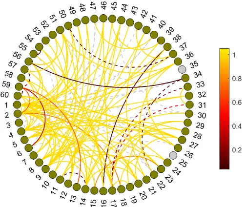
infer-Figure 2: Plot of Simulation 3. The estimated graph based on the marginal inclusion prob-ability for each edge.
ence results are compared with the other three methods in the bottom panel of Table 1. Similar patterns are observed as in Simulation 1. In particular, the proposed functional data graphical model shows a clear advantage in accurately estimating the graph. Estimates of the functions{fij}and their time-domain correlations are provided in the online appendix.
4.3 Simulation 3: Graph Estimation When p is Greater than n
To further investigate the performance of the proposed approach when the number of nodesp is greater than the sample sizen, we design another simulation study with p= 60 and n = 55. The true graph contains 60 nodes, among which 2 are singletons and 58 are connected with edges. The total number of edges in the true graph is 121. Smooth functional data are simulated following the procedure described in Section 4.1. With the simulated data, we apply the PACE algorithm to estimate{ci}and determine the truncation parameters using the FVE criterion with a 95% threshod. We then apply Algorithm 1 and set prior parameters δ and U following Simulation 1. Posterior samples of the graph are obtained for 30,000 MCMC iterations after removing 10,000 burn-in samples.
simulations, resulting in mean mis-estimation rate 0.02, sensitivity 0.77, and specificity 0.99. Extra simulation runs show that the sensitivity level is improved when we increase the sample size n.
5. Analysis of Event-related Potential Data in an Alcoholism Study
We apply the proposed method to event-related potential data from an alcoholism study. Data were initially obtained from 64 electrodes placed on subjects’ scalps that captured EEG signals at 256 Hz during a one-second period. The measurements were taken from 122 subjects, of which 77 belonged to the alcoholism group and 45 to the control group. Each subject completed 120 trials. During each trial, the subject was exposed to either a single stimulus (a single picture) or two stimuli (a pair of pictures) shown on a computer monitor. We band-pass filtered the EEG signals to extract the α frequency band in the range of 8–12.5 Hz. The filtering was performed by applying the eegfilt function in the EEGLAB toolbox of Matlab. Theα-band signal is known to be associated with inhibitory control (Knyazev, 2007). Research has shown that, relative to control subjects, alcoholic subjects demonstrate unstable or poor rhythm and lower signal power in the α-band signal (Porjesz et al., 2005; Finn and Justus, 1999), indicating decreased inhibitory control (Sher et al., 2005). Moreover, regional asymmetric patterns have been found in alcoholics— alcoholics exhibit lower left α-band activities in anterior regions relative to right (Hayden et al., 2006). In this study, we aim to estimate the conditional independence relationships of α-band signals from different locations of the scalp, and expect to find evidence that reflects differences in brain connectivity and asymmetric pattern between the two groups.
Since multiple trials were measured over time for each subject, the EEG measurements may not be treated as independent due to the time dependence of the trials. Furthermore, since the measurements were taken under different stimuli, the signals could be influenced by different stimulus effects. To remove the potential dependence between the measurements and the influence of different stimulus types, for each subject, we averaged the band-filtered EEG signals across all trials under the single stimulus, resulting in one Event-related po-tential (ERP) curve per electrode per subject. ERP is a type of electrophysiological signal generated by averaging EEG segments recorded under repeated applications of a stimu-lus, with the averaging serving to reduce biological noise levels and enhance the stimulus evoked neurological signal (Brandeis and Lehmann, 1986; Bressler, 2002). Based on the preprocessed ERP curves, we further removed subjects with missing nodes, and balanced the sample size across the two groups, producing multivariate functional data with n= 44 andp= 64 for both the alcoholic and the control group. We applied model (4) using coeffi-cients of the eigenbasis expansion. The number of eigenbasis{Mj}was determined through
retaining 90% of the total variation; this resulted in 4–7 coefficients per fj. We collected
30,000 posterior samples using Algorithm 1, in which the first 10,000 were treated as the burn-in period. The model was fitted for both the alcoholic and the control group, and convergence of the MCMC was justified by running multiple chains starting with various initial values.
Figure 3: Summary of posterior inference: the marginal inclusion probabilities for edges in the alcoholic group (a) and the control group (b); the boxplots of connectivity measures: the number of edges connecting with nodes in the frontal and parietal regions (c), and the overall total number of edges (d); the boxplots of asymmetry measures: the number of asymmetric edges for nodes in the frontal and the parietal regions (e), and the overall total number of asymmetric edges (f). In (a) and (b), the edge color indicates the magnitude of the posterior inclusion probability. In (c)–(f), the alcoholic group is abbreviated as “al”, and the control group is abbreviated as “ct”.
To further compare with established results, we calculated two summary statistics for connectivity: the number of edges connected with nodes in a specific region, and the overall total number of edges. We also calculated two additional summary statistics for asymmetry: the number of asymmetric edges for all nodes in a specific region, and the overall total number of asymmetric edges. We summarized these summary statistics across the two groups using boxplots in Figure 3 (c)–(f), and calculated the posterior probability that the alcoholic group is greater than, equal to, or less than the control group for each statistic. Results show that, with probability≈1, the alcoholic group has fewer edges than the control group in the frontal and the parietal region, and has fewer overall total number of edges; with probability 0.95, the alcoholic group has more asymmetric edges than the control group in the frontal region; and with probability≈1, the alcoholic group has higher overall total number of asymmetric edges than the control group. These results indicate that the alcoholic group exhibits decreased regional and overall connectivity, increased asymmetry in the frontal region, and increased overall asymmetry. These observations are consistent with the findings of Hayden et al. (2006), who studied the asymmetric patterns at two frontal electrodes (F3, F4) and two parietal electrodes (P3, P4) using the analysis of variance method based on the resting-state α-band power. In comparison, our analysis provides connectivity and asymmetric pattern of all 64 electrodes simultaneously whereas Hayden et al. (2006) only focuses on the four representative electrodes.
6. Discussion
We have constructed a theoretical framework for graphical models of multivariate func-tional data and proposed a HIWP prior for the special case of Gaussian process graphical models. For practical implementation, we have suggested a posterior inference approach based on a regularization condition, which enables posterior sampling through MCMC al-gorithms.
One concern is whether it is possible to perform exact posterior inference without the regularity condition on approximation, i.e., inferring the graph directly from the joint pos-terior p(G|{ci}) ∝ p({ci}|G)p(G) based on model (4), where p({ci}|G) is the marginal likelihood (with the covariance kernelQC integrated out) andp(G) is the prior distribution
for G. Although the above joint posterior is theoretically well-defined according to Theo-rem 2, exact posterior sampling is difficult due to the fact that the density function for the marginal likelihood can only be calculated on a finite dimensional projection of {ci}.
more complicated because the dimension of the truncated sequences and the size of the covariance matrixQC would change whenever M is updated.
We have demonstrated the application of the proposed approach through an ERP data set. By treating ERPs as functional data, we are estimating the systematic brain connec-tivity that is common across a group of subjects and a time interval. For other modeling purposes, such as estimating the individual level or dynamic brain connectivity, one could use multivariate graphical models described in Carvalho and West (2007) or Bilmes (2010). We have focused on decomposable graphs. In case of non-decomposable graphs, the proposed HIWP prior may still apply if we replace the inverse-Wishart process prior for each clique with that for a prime component of the graph. For a non-complete prime component P, the inverse-Wishart processes prior for QP is subject to extra constraint induced by missing edges.
We have applied the proposed method to graphs of small to moderate size, with number of nodes as large as 60. To deal with larger scale problems (e.g, multivariate functional data with hundreds or thousands of functional components), more efficient large-scale compu-tational techniques such as the fast Cholesky factorization (Li et al., 2012) can be readily combined with our MCMC algorithms. Furthermore, non-MCMC algorithms may be more computationally efficient in case of large graphs. For example, based on the posterior dis-tribution ofGin (8), a fast search algorithm may be developed to search for the maximum a posteriori (MAP) solution following ideas similar to Daum´e III (2007) and Jalali et al. (2011).
Acknowledgments
Appendix A. Definitions
Definitions used in the lemmas, theorems and their proofs are listed as follows: (I)
Projection map. Let R be the real line and T be an index set. Consider the
Carte-sian product space RT×T = Q(α,β)∈T×T R(α,β). For a fixed point (α, β) ∈ T ×T, we
define the projection map π(α,β) : RT×T → R(α,β) as π(α,β) {x(l,m): (l, m)∈T ×T}
= x(α,β). For a subset B ⊂ T ×T, we define the partial projection πB : RT×T → RB as
πB {x(l,m): (l, m)∈T×T}
= {x(s,t) : (s, t) ∈ B}. More generally, for subsets B1, B2,
such that B2 ⊂ B1 ⊂ T ×T, we define the partial sub-projections πB2←B1 : R B1 →
RB2,
by πB2←B1({x(l,m) : (l, m) ∈ B1}) = {x(s,t) : (s, t) ∈ B2}. (II) The pullback of a σ -algebra. Let B(α,β) be a σ-algebra on R(α,β). We can create a σ-algebra on RT×T by
pulling back the B(α,β) using the inverse of the projection map and defineπ∗(α,β)(B(α,β)) =
{π−(α,β)1 (A) : A ∈ B(α,β)}. One can verify that π∗(α,β)(B(α,β)) is a σ-algebra. (III) Prod-uct σ-algebra. We define the product σ-algebra as B(RT×T) = Q(α,β)∈T×T B(α,β), where
Q
(α,β)∈T×T B(α,β) = σ
S
(α,β)∈T×T π∗(α,β)(B(α,β))
. (IV) Pushforward measure. Given a measure µT×T on the product σ-algebra, and a subset B of T ×T, we define the
push-forward measure µB = (πB)∗µT×T on RB as µB(A) = µT×T{πB−1(A)} for all A ∈ BB,
where BB =Q(α,β)∈BB(α,β). (V) Compatibility. Given subsets B1, B2 of T ×T such that
B2 ⊂B1 ⊂T ×T, the pushforward measures µB1 and µB2 are said to obey compatibility
relation if (πB2←B1)∗µB1 =µB2.
Appendix B. Proof of Lemma 1
This proof involves some measure-theoretic arguments. The essential idea is to use disintegration theory Chang and Pollard (1997) to first construct the conditional probability measureP1{· |πA∩B(fA)}onB(L2(TA)), extend this toP{ · |πB(f)}onB(L2(TA∪B)), and
finally construct the joint measure P which satisfies conditions (i)–(iii).
Denote TA = Fj∈ATj. Since P1 is a finite Radon measure and the projection πA∩B :
L2(TA)→L2(TA∩B) is measurable, we invoke the disintegration theorem to obtain measures
P1{· |πA∩B(fA)} on B(L2(TA)) satisfying:
(a.1) P1(X |fA∩B) =P1
X ∩[L2(TA\B)× {πA∩B(fA)}]|πA∩B(fA) for allX ∈ B(L2(TA)),
(b.1) the map fA∩B 7→ (P1)fA∩BH : =
Z
H(fA)dP1(fA |fA∩B) is measurable for all
non-negative measurableH :L2(TA)→R,
(c.1) P1H = ((πA∩B)∗P1)(P1)fA∩BH for all nonnegative measurable H : L 2(T
A) → R,
where (πA∩B)∗P1 is the push-forward measure of P1.
Now, we define the measureP{· |πB(f)}by settingP{A |πB(f)}=P1{πA(A∩[L2(TA\B)×
{πB(f)}]) | πA∩B(f)}. Note that this is well defined for all measurable A ∈ B(L2(TA∪B))
since the sections πA(A ∩[L2(TA\B)× {πB(f)}]) are always measurable, and also that (a)
P{A |πB(f)}=P{A ∩[L2(TA\B)× {πB(f)}]|πB(f)} holds by construction. Now, let M
denote the set of measurable functions from L2(TA∪B) to R satisfying (b) fB 7−→ PfBH
suppose Hn is a sequence of positive measurable functions in M increasing pointwise to
a bounded measurable function H. For each fixed fB in L2(TB), we then have that
Hn is a sequence of positive measurable functions increasing pointwise to H, and hence
the monotone convergence theorem implies PfBHn −→ PfBH in an increasing manner.
Since this holds for each fB, we conclude that PfBH is the point-wise increasing limit of
measurable functions on L2(TB), and hence it is measurable. Moreover, it is simple to
see that PfB1X ×Y = P1(X | fA∩B)1Y(fB\A) is a measurable function on L 2(T
B) for all
X ∈ B(L2(TA)) andY ∈ B(L2(TB\A)), and hence1X ×Y ∈ M. By the Monotone Class
The-orem, we then have that all bounded measurable functions on L2(TA∪B) satisfy (b), and
hence it will hold for all positive measurable functions onL2(TA∪B). Since (b) is satisfied
for all positive measurable functions, we may define the measure P H =P2PfBH. By
con-struction, we have that P1L2(TA\B)×Y =P2P1(L2(TA\B)× {fA∩B} |fA∩B)1Y(fB) =P2(Y)
and P1X ×L2(TB\A) = P2P1(X | fA∩B) = ((πA∩B)∗P2)P1(X | fA∩B) = ((πA∩B)∗P1)P1(X | fA∩B) =P1(X).Thus, we also have that P H = P2PfBH = ((πB)∗P)PπB(f)H for all
mea-surableH, and this is the final property establishing thatP(· |fB) is a disintegration ofP
with respect to the mapπB. By the disintegration theorem, this disintegration is a version
of the regular conditional probability offAgiven fB. Since this version only depends upon fA∩B, we conclude that (iii) holds. Finally, we note that any other measure satisfying these
properties must agree with the measure we have constructed on π-system, and therefore
the uniqueness ofP immediately follows.
Appendix C. Proof of Proposition 1
Proof. The Properties 1 - 4 in Dawid and Lauritzen (1993) are treated as axioms; they are universal properties thus also hold when X, Y, Z are random processes. Since the graphGis undirected and decomposable, the results on graphical theory in Appendix A of Dawid and Lauritzen (1993) continue to hold. Properties 1 - 4 and results in Appendix A imply that results in B1- B7 of Dawid and Lauritzen (1993) continue to hold when P is a Markov distribution constructed in Lemma 1. Theorem 2.6 and Corollary 2.7 of Dawid and Lauritzen (1993) are also implied. These results, combined with the definition of marginal distribution defined by pushforward measure and the definition of conditional probability measure based on disintegration theory, prove that Lemmas 3.1, 3.3, Theorems 3.9 - 3.10 as well as Propositions 3.11, 3.13, 3.15, 3.16, 3.18 from Dawid and Lauritzen (1993) hold.
Appendix D. Lemma 2 and Proof
Lemma 2 Let N be the set of positive integers and I an arbitrary finite subset of it.
Suppose that δ > 4 is a positive integer and that u :N×N → R is a symmetric positive
semidefinite and trace class kernel so that the matrix UI×I formed by {u(i, j), i, j ∈ I}
is symmetric positive semidefinite. Then there exists a unique probability measure µ on (RN×N,B(RN×N)) satisfying
i. (πI×I)∗µ=µI×I, whereµI×I is the law of IW(δ,UI×I) defined in Dawid (1981);
ii. if B ={(αi, βi)}ni=1 ⊂N×N and g ={αi}ni=1∪ {βi}ni=1, then (πB)∗µ=µB, where
Setting µ=IWP(δ,U) so that (U)ij =u(i, j), we further have that if Q∼IWP(δ,U) and
δ >4, the countably infinite arrayQis a positive semidefinite trace class operator on`2(N)
almost surely.
Proof. Let UI×I be a matrix with the law µI×I. We will prove following Tao (2011,
Theorem 2.4.3) as follows: (1) we verify the compatibility ofµB for all finite B ⊂N×N.
There are two successive cases we shall consider. Case 1: Suppose I2 ⊂ I1 are two finite
subsets of N, then QI2×I2 is the sub-matrix of QI1×I1 obtained by deleting the rows and
columns with indices in I1 \I2. If QI1×I1 has law µI1×I1 = IW(δ,UI1×I1), then QI2×I2
has law IW(δ,UI2×I2) due to the consistency property of the inverse-Wishart distribution
(Dawid and Lauritzen, 1993, Lemma 7.4). Consequently, (πI2×I2←I1×I1)∗µI1×I1 =µI2×I2.
Case 2: Let B1 = {(αi, βi)}ni=1 ⊂ N×N and suppose B2 = {(αei,βei)}
m
i=1 ⊂ B1. Set
g1 ={αi}ni=1∪ {βi}ni=1 and g2={αei}
m
i=1∪ {βei}mi=1 so that g2×g2 ⊂g1×g1. It is clear that πB2←B1 ◦πB1←g1×g1 =πB2←g1×g1 =πB2←g2×g2 ◦πg2×g2←g1×g1.Thus,
(πB2←B1)∗µB1 = (πB2←B1)∗(πB1←g1×g1)∗µg1×g1 = (πB2←B1◦πB1←g1×g1)∗µg1×g1
= (πB2←g2×g2◦πg2×g2←g1×g1)∗µg1×g1 = (πB2←g2×g2)∗(πg2×g2←g1×g1)∗µg1×g1
= (πB2←g2×g2)∗µg2×g2 =µB2,
where the second to last equality holds because of our demonstration in Case 1. (2) Second, we claim that the finite dimensional measure µI×I =IW(δ,UI×I) is an inner regular
prob-ability measure on the product σ-algebra BI×I. We will show that µI×I is a finite Borel
measure on a Polish space, which then implies thatµI×I is regular, hence inner regular by
Bauer (2001, Lemma 26.2). This is done through (a)–(c) as follows: (a) For finite I,QI×I
takes values in the space of symmetric and positive semidefinite matrices, denoted by Ψ|I|
where |N|denotes the number of elements in I. Since the subset of symmetric matrices is closed inRI×I, it is Polish. Furthermore, the space of symmetric positive semidefinite
ma-trices is an open convex cone in the space of symmetric mama-trices, hence it is Polish as well. Therefore the space Ψ|I| is Polish. (b) Since µI×I, the law of QI×I ∼IW(δ, UI×I), has an
almost everywhere continuous density function,µI×I is a measure defined by Lebesgue
inte-gration against an almost everywhere continuous function. ThereforeµI×I is Borel on Ψ|I|.
As Ψ|I|⊂RI×I, we may extend the measureµI×I from Ψ|I| toRI×I via the Carath´eodory
theorem (Tao, 2011, Theorem 1.7.3). In particular, define µeI×I(A) = µI×I(A∩Ψ|I|) for
A ∈ B(RI×I). With extension, µI×I is Borel on RI×I, and the σ-algebra associated is
B(RI×I) =BI×I =Q(α,β)∈I×IB(α,β). (c) The measureµI×I is certainly finite since it is a
probability measure.
The compatibility and regularity conditions in (1) and (2) ensure that the Kolmogorov extension theorem holds. Therefore there exists a unique probability measure µ on the productσ-algebra B(RN×N) that satisfies (i) and (ii).
We now prove that if Q ∼ IWP(δ,U), then the countably infinite array Q is a well-defined positive semidefinite trace class operator on`2(N) almost surely. First, we note that
the spectral theorem ensures the existence of an orthonormal basis of`2(N) that diagonalizes
U. Thus, without loss of generality, we may assume thatQis drawn fromIWP(δ,U) where
U is a diagonal positive semidefinite trace class operator on`2(N).
First, we show each row of Qx is finite almost surely hence is well-defined for all x ∈
qii qij
qij qjj
∼IW
δ,
uii 0
0 ujj
and hence using the moments of finite dimensional
inverse-Wishart,E(q2ii) =u2ii(δ−2)−1(δ−4)−1, E(q2ij) =uiiujj(δ−1)−1(δ−2)−1(δ−4)−1,
for δ > 4. By Tonelli’s theorem, we have that EP
jq2ij =
P
jEq2ij ≤ C
P
juiiujj =
CuiiPjujj, whereC is the maximum of the above constants. Thus
E[|(Qx)i|]≤ kxk
s EX
j
q2 ij <∞.
Because there are only countably many rows, we have thatQxis finite almost surely for all rows simultaneously. Consequently, we have thatQx is well-defined for allx∈`2(N). Now
we show that Qx ∈ `2(
N) almost surely. By similar considerations, let qi = (Qx)i, then
E(P
ikqik2)≤C(
P
iuii) 2
<∞andkQxk2 ≤Ckxk2P
ikqik2; this implies thatkQxk<∞
almost surely hence Qx ∈`2(N) almost surely, and it also implies that the operator norm
kQkop is finite almost surely.
By construction, we must have that Q is positive semidefinite almost surely since
hQx,xi = limn→∞hQnx,xi ≥ 0, where Qn is the restriction of Q to its n by n leading
principal minor. Finally, Q is trace class almost surely since E[|tr(Q)|] = P
iE(qii) =
(δ−2)−1P
iuii<∞.
Appendix E. Proof of Theorem 1
Proof. Based on Lemma 2, we can define a sequence of inverse-Wishart process prior for
QC, denoted by QC ∼ IWP(δ,UC), C ∈ C. These sequences are pairwise consistent due to the consistency of inverse-Wishart processes and the fact thatUC is a common collection of
kernels. Therefore, we can construct a unique hyper Markov law forQCfollowing procedure
(12) - (13) of Dawid and Lauritzen (1993). And Theorem 3.9 of Dawid and Lauritzen (1993)
guarantees that the constructed hyper Markov law is unique.
Appendix F. Proof of Proposition 2
Proof. Note that an operator drawn from a hyper-inverse-Wishart process with the parameter U satisfies rank(uij) <∞ fori, j ∈V will have finite-rank almost surely. This
follows by noting that if Q ∼ HIWP(δ,U) and W is a fixed unitary transformation on `2, then WTQW ∼ HIWP(δ,WTU W). Thus, choosing W so that the block representation
WTU W =
U 0
0 0
holds (here, U is a finite matrix and 0’s represent infinite arrays of
zeros), we see that the block representation WTQW =
Q 0
0 0
holds almost surely, and
that Q∼IW(δ, U). Consequently, we have reduced to the finite-dimensional setting where
the result is well-known.
Appendix G. Proof of Theorem 2
Proof. By the result of Proposition 1, the HIWPG prior is a strong hyper Markov law.
hyper Markov law specified by the marginal posterior laws at each clique. In other words, we just need to find the posterior law for the model: ci,C ∼ dMGP(c0,C,QC) with prior
QC ∼IWP(δ,UC) for eachQC, and use them to construct the posterior law ofQC following
(12) - (13) of Dawid and Lauritzen (1993). As in the last proof, choosing an appropriate transformation reduces this to the finite-dimensional case which is well-known. Finally, by Proposition 5.6 of Dawid and Lauritzen (1993), the marginal distribution of {ci} given
G,c0, δ,UeC is again Markov over G.
Online Appendix
The online appendix contains more detailed derivations, discussions, and simulation results.
References
A. Anandkumar, V. Y. F. Tan, F. Huang, and A. S. Willsky. High-dimensional structure estimation in Ising models: local separation criterion. Ann. Statist., 40(3):1346–1375, 06 2012.
H. Bauer. Measure and Integration Theory. De Gruyter Studies in Mathematics. W. de Gruyter, 2001.
J. Bilmes. Dynamic graphical models.IEEE Signal Processing Magazine, 27(6):29–42, 2010.
D. Brandeis and D. Lehmann. Event-related potentials of the brain and cognitive processes: approaches and applications. Neuropsychologia, pages 151–168, 1986.
S. L. Bressler. Event-related potentials. In M.A. Arbib, editor, The Handbook of Brain Theory and Neural Networks, pages 412–415. MIT Press, Cambridge MA, 2002.
T. Cai, W. Liu, and X. Luo. A constrained l1 minimization approach to sparse precision matrix estimation. J. Amer. Statist. Assoc., 106(494):594–607, 2011.
C. M. Carvalho and J. G. Scott. Objective Bayesian model selection in Gaussian graphical models. Biometrika, 96(3):497–512, 2009.
C. M. Carvalho and M. West. Dynamic matrix-variate graphical models. Bayesian Anal., 2(1):69–98, 2007.
J. T. Chang and D. Pollard. Conditioning as disintegration. Statistica Neerlandica, 51(3): 287–317, 1997.
H. Daum´e III. Fast search for dirichlet process mixture models. In Eleventh International Conference on Artificial Intelligence and Statistics (AIStats), 2007.
A. P. Dawid. Some matrix-variate distribution theory: Notational considerations and a Bayesian application. Biometrika, 68(1):265–274, 1981.
C. De Boor. A Practical Guide to Splines. Applied Mathematical Sciences. Springer, Berlin, 2001.
A. P. Dempster. Covariance selection. Biometrics, 28:157–175, 1972.
P. R. Finn and A. Justus. Reduced EEG alpha power in the male and female offspring of alcoholics. Alcohol. Clin. Exp. Res., 23:256–262, 1999.
J. Friedman, T. Hastie, and R. Tibshirani. Sparse inverse covariance estimation with the graphical lasso. Biostatistics, 9(3):432–441, 2008.
P. Giudici. Learning in graphical Gaussian models. Bayesian Statistics 5, pages 621–628, 1996.
P. Giudici and P. J. Green. Decomposable graphical Gaussian model determination.
Biometrika, 86(4):785–801, 1999.
Y. Guan and S. M. Krone. Small-world MCMC and convergence to multi-modal distribu-tions: From slow mixing to fast mixing. Ann. Appl. Prob., 17:284–304, 2007.
Y. Guan, R. Fleissner, P. Joyce, and S. M. Krone. Markov chain Monte Carlo in small worlds. Stat. Comput., 16:193–202, 2006.
E. P. Hayden, R. E. Wiegand, E. T. Meyer, L. O. Bauer, S. J. O’Connor, J. I. Nurnberger, D. B. Chorlian, B. Porjesz, and H. Begleiter. Patterns of regional brain activity in alcohol-dependent subjects. Alcohol. Clin. Exp. Res., 30(12):1986 – 1991, 2006.
H. H¨ofling and R. Tibshirani. Estimation of sparse binary pairwise Markov networks using pseudo-likelihoods. J. Mach. Learn. Res., 10:883–906, 2009.
A. Jalali, C. C. Johnson, and P. K. Ravikumar. On learning discrete graphical models using greedy methods. In J. Shawe-taylor, R.s. Zemel, P. Bartlett, F.c.n. Pereira, and K.q. Weinberger, editors, Advances in Neural Information Processing Systems 24, pages 1935–1943. 2011.
M. Jansen and P. J. Oonincx. Second Generation Wavelets and Applications. Springer-Verlag, London, 2015.
B. Jones, C. Carvalho, A. Dobra, C. Hans, C. Carter, and M. West. Experiments in stochastic computation for high-dimensional graphical models. Statist. Sci., 20(4):388– 400, 2005.
Gennady G. Knyazev. Motivation, emotion, and their inhibitory control mirrored in brain oscillations. Neurosci. Biobehav. Rev., 31(3):377 – 395, 2007.
M. Kolar and E. Xing. On time varying undirected graphs. J. Mach. Learn. Res., 15: 407–415, 2011.
S. L. Lauritzen. Graphical Models. Clarendon Press, Oxford, 1996.
E. Lei, F. Yao, N. Heckman, and K. Meyer. Functional data model for genetically related individuals with application to cow growth. J. Comp. and Graph. Stat., 2014.
S. Li, M. Gu, C. J. Wu, and J. Xia. New efficient and robust HSS Cholesky factorization of SPD matrices. SIAM J. Matrix Anal. Appl., pages 886–904, 2012.
P-L. Loh and M. J. Wainwright. Structure estimation for discrete graphical models: Gen-eralized covariance matrices and their inverses. Ann. Statist., 41(6):3022–3049, 12 2013.
P. Ma, C. I. Castillo-Davis, W. Zhong, and J. S. Liu. A data-driven clustering method for time course gene expression data. Nucleic Acids Res., 34(4):1261–1269, 2006.
R. Mazumder and T. Hastie. The graphical lasso: New insights and alternatives. Electron. J. Statist., 6:2125–2149, 2012a.
R. Mazumder and T. Hastie. Exact covariance thresholding into connected components for large-scale graphical lasso. J. Mach. Learn. Res., 13:781–794, 2012b.
N. Meinshausen and P. B¨uhlmann. High dimensional graphs and variable selection with the Lasso. Ann. Statist., 34(3):1436–1462, 2006.
H. G. M¨uller and F. Yao. Functional additive models.J. Am. Statist. Assoc., 103:1534–1544, 2008.
B. Porjesz, M. Rangaswamy, C. Kamarajan, K. A. Jones, A. Padmanabhapillai, and H. Be-gleiter. The utility of neurophysiological markers in the study of alcoholism. Clin. Neu-rophysiol., 116(5):993 – 1018, 2005.
G. D. Prato. An Introduction to Infinite-Dimensional Analysis. Springer, New York, 2006.
X. Qiao, G. James, and J. Lv. Functional graphical models. Technical report, University of Southern California, 2015.
J. O. Ramsay and B. W. Silverman. Functional Data Analysis, Section Edition. Springer, New York, 2005.
P. Ravikumar, M. J. Wainwright, and J. D. Lafferty. High-dimensional Ising model selection using l1-regularized logistic regression. Ann. Statist., 38(3):1287–1319, 06 2010.
J. A. Rice and B. W. Silverman. Estimating the mean and covariance structure nonpara-metrically when the data are curves. J. R. Stat. Soc., Series B, 53:233–243, 1991.
A. Roverato. Hyper inverse Wishart distribution for non-decomposable graphs and its application to Bayesian inference for Gaussian graphical models. Scand. J. Stat., 29: 391–411, 2002.
J. G. Scott and C. M. Carvalho. Feature-inclusion stochastic search for Gaussian graphical models. J. Comput. Graph. Statist., 17(4):790–808, 2008.
K. J. Sher, E.R. Grekin, and N. A. Williams. The development of alcohol use disorders.
Annu. Rev. Clin. Psychol., 1:493–523, 2005.
T. Tao. An Introduction to Measure Theory. Graduate Studies in Mathematics. Amer. Math. Soc., 2011.
H. Wang and M. West. Bayesian analysis of matrix normal graphical models. Biometrika, 96(4):821–834, 2009.
D. M. Witten, J. H. Friedman, and N. Simon. New insights and faster computations for the graphical Lasso. J. Comp. Graph. Stat., 20(4):892–900, 2011.
E. Yang, G. Allen, Z. Liu, and P. K. Ravikumar. Graphical models via generalized linear models. In F. Pereira, C.J.C. Burges, L. Bottou, and K.Q. Weinberger, editors,Advances in Neural Information Processing Systems 25, pages 1358–1366. Curran Associates, Inc., 2012.
F. Yao, H. G. M¨uller, and J. L. Wang. Functional data analysis for sparse longitudinal data. J. Am. Statist. Assoc., 100:577–590, 2005.
M. Yuan and Y. Lin. Model selection and estimation in the Gaussian graphical model.
Biometrika, 94:19–35, 2007.