Generalized Conditional Gradient for Sparse Estimation
Yaoliang Yu [email protected]
School of Computer Science University of Waterloo
Waterloo, ON, N2L 3G1, Canada
Xinhua Zhang [email protected]
Department of Computer Science University of Illinois at Chicago Chicago, IL 60607
Dale Schuurmans [email protected]
Department of Computing Science University of Alberta
Edmonton, Alberta T6G 2E8, Canada
Editor:Koby Crammer
Abstract
Sparsity is an important modeling tool that expands the applicability of convex formula-tions for data analysis, however it also creates significant challenges for efficient algorithm design. In this paper we investigate the generalized conditional gradient (GCG) algorithm for solving sparse optimization problems—demonstrating that, with some enhancements, it can provide a more efficient alternative to current state of the art approaches. After study-ing the convergence properties of GCG for general convex composite problems, we develop efficient methods for evaluating polar operators, a subroutine that is required in each GCG iteration. In particular, we show how the polar operator can be efficiently evaluated in learning low-rank matrices, instantiated with detailed examples on matrix completion and dictionary learning. A further improvement is achieved by interleaving GCG with fixed-rank local subspace optimization. A series of experiments on matrix completion, multi-class classification, and multi-view dictionary learning shows that the proposed method can sig-nificantly reduce the training cost of current alternatives.
Keywords: generalized conditional gradient, frank-wolfe, dictionary learning, matrix completion, multi-view learning, sparse estimation
1. Introduction
Sparsity is an important concept in high-dimensional statistics (B¨uhlmann and van de Geer, 2011) and signal processing (Eldar and Kutyniok, 2012), which has led to important application successes by reducing model complexity and improving interpretability of the results. Although it is common to promote sparsity by adding appropriate regularizers, such as the l1 norm, sparsity can also present itself in more sophisticated forms, such as group
sparsity (Yuan and Lin, 2006), graph sparsity (Kim and Xing, 2009; Jacob et al., 2009), matrix rank sparsity (Cand`es and Recht, 2009), and other combinatorial sparsity patterns (Obozinski and Bach, 2012). These recent notions ofstructured sparsity (Bach et al., 2012;
c
Micchelli et al., 2013) have greatly enhanced the ability to model structural relationships in data; however, they also create significant computational challenges.
A currently popular optimization scheme for training sparse models isaccelerated prox-imal gradient (APG) (Beck and Teboulle, 2009; Nesterov, 2013), which enjoys an optimal rate of convergence among black-box first-order procedures (Nesterov, 2013). An advan-tage of APG is that each iteration consists solely of computing a proximal update (PU), which for simple regularizers can have a very low complexity. For example, underl1 norm regularization each iterate of APG reduces to a soft-shrinkage operator that can be com-puted in linear time, which partly explains its popularity for such problems. Unfortunately, for matrix low-rank regularizers the PU soon becomes a computational bottleneck. For example, the trace norm is often used to promote low rank solutions in matrix variable problems such as matrix completion (Cand`es and Recht, 2009); but here the associated PU requires afull singular value decomposition (SVD) of the gradient matrix on each iteration, which prevents APG from being applied to large problems. Not only does the PU require nontrivial computation for matrix regularizers, it also yields dense intermediate iterates.
To address the primary shortcomings with APG, we investigate the generalized condi-tional gradient (GCG) strategy for sparse optimization, which has been motivated by the promise of recent sparse approximation methods (Hazan, 2008; Clarkson, 2010). A special case of GCG, known as the conditional gradient (CG), was originally proposed by Frank and Wolfe (1956) and has received significant renewed interest (Bach, 2015; Clarkson, 2010; Fre-und and Grigas, 2016; Hazan, 2008; Jaggi and Sulovsky, 2010; Jaggi, 2013; Shalev-Shwartz et al., 2010; Tewari et al., 2011; Yuan and Yan, 2013). The key advantage of GCG for sparse estimation is that it need only compute thepolar of the regularizer in each iteration, which sometimes admits a much more efficient update than the PU in APG. For example, under trace norm regularization, GCG only requires the spectral norm of the gradient to be computed in each iteration, which is an order of magnitude cheaper than evaluating the full SVD as required by APG. Furthermore, the greedy nature of GCG affords explicit control over the sparsity of intermediate iterates, which is not available in APG. Although existing work on GCG has generally been restricted to constrained optimization (i.e. en-forcing an upper bound on the sparsity-inducing regularizer), in this paper we consider the more general regularized version of the problem. Despite their theoretical equivalence, the regularized form allows more efficient local optimization to be interleaved with the primary update, which provides a significant acceleration in practice.
This paper is divided into two major parts: first we present a general treatment of GCG and establish its convergence properties for convex optimization in Section 3, with a special focus on convex gauge regularizers; then we apply the method to important case studies to demonstrate its effectiveness on large-scale, sparse estimation problems in Section 4, with experiments presented in Section 5.
algorithms demonstrate alternative trade-offs between the number of iterations required and the per-step complexity. As shown in our experiments, GCG can be significantly faster than APG in terms ofoverall computation time for large problems. The results in Section 3 are new.
Equipped with the technical results of GCG on convex optimization, the second part of the paper then applies the algorithm to the important application of low rank learning (Section 4). Since imposing a hard bound on matrix rank generally leads to an intractable problem, in Section 4.2 we first present a generic relaxation strategy based on convex gauges (Chandrasekaran et al., 2012; Tewari et al., 2011) that yields a convex program (Bach et al., 2008; Bradley and Bagnell, 2009; Zhang et al., 2012). Conveniently, the resulting problem can be easily optimized using the GCG algorithm from Section 3.2. To further reduce com-putation time, we introduce in Section 4.3 an auxiliary fixed rank subspace optimization within each iteration of GCG. Although similar hybrid approaches have been previously suggested (Burer and Monteiro, 2005; Laue, 2012; Mishra et al., 2013), we propose an effi-cient new alternative that, instead of locally optimizing a constrained fixed rank problem, optimizes anunconstrained surrogate objective based on a variational representation of ma-trix norms. This alternative strategy allows a far more efficient local optimization without compromising GCG’s convergence properties. In Section 4.4 we show that the approach can be applied to dictionary learning and matrix completion problems, as well as a non-trivial multi-view form of dictionary learning (White et al., 2012).
Finally, in Section 5 we provide an extensive experimental evaluation that compares the performance of GCG (augmented with interleaved local search) to state-of-the-art op-timization strategies, across a range of problems, including matrix completion, multi-class classification, and multi-view dictionary learning.
1.1 Extensions over Previously Published Work
Some of the results in this article have appeared in a preliminary form in two conference papers (Zhang et al., 2012; White et al., 2012); however, several specific extensions have been added in this paper, including:
• A more extensive and unified treatment of GCG in general Banach spaces.
• A more refined analysis of the convergence properties of GCG.
• A new application of GCG to multi-view dictionary learning.
• New experimental evaluations on larger data sets, including new results for matrix completion and image multi-class classification.
• Open source Matlab code released at https://www.cs.uic.edu/~zhangx/GCG.
2. Preliminaries
2.1 Notation and Definitions
Throughout this paper we assume that the underlying space, unless otherwise stated, is a real Banach space B with norm k·k; for example, B could be the Euclidean space Rd with any norm. The dual space (the set of all real-valued continuous linear functions on B) is denoted B∗ and is equipped with the dual normkgk◦ = sup{g(w) :kwk ≤ 1}. Note that for a differentiable function f :B → R:= R∪ {∞}, its (Frech´et) derivative ∇f is in the dual spaceB∗.
We use bold lowercase letters to denote vectors, where the i-th component of a vector wis denotedwi, whilewtdenotes some other vector. We use the shorthandhw,gi:=g(w)
for any g ∈ B∗ and w ∈ B. We call a function f : B → R σ-strongly convex (w.r.t. the norm k·k) if there exists some σ≥0 such that for all 0≤λ≤1 and w,z∈ B,
f(λw+ (1−λ)z) +12σλ(1−λ)kw−zk2≤λf(w) + (1−λ)f(z). (1) In the case where σ = 0 we simply say f is convex. A setC ⊆ B is called convex if for all w,z∈C =⇒ λw+ (1−λ)z∈C for all 0≤λ≤1. It follows from the definition that the domain of a convex function f, denoted as domf :={w:f(w)<∞}, is a convex set. The functionf is called proper if domf 6=∅, and closed if all sublevel sets {w:f(w)≤α} are closed for allα∈R. The subdifferential of a convex functionf :B →Ratwis defined as the set ∂f(w) ={g∈ B∗:f(z)≥f(w) +hz−w,gi,∀z∈ B}.
Key to our subsequent development is two particular functions associated with a nonempty set in B: the indicator function
ιC(w) = (
0, ifw∈C
∞, otherwise, (2)
and the gauge function
κ(w) =κA(w) := inf{ρ≥0 :w∈ρA}, (3)
where ρA := {ρw : w ∈ A}, and the infimum is taken to be infinity over an empty set (i.e. when the condition w ∈ ρA is not satisfied for any ρ ≥ 0). Intuitively, κ(w) is the smallest rescaling of the set A to “barely” contain w; see Figure 1. Note that we always haveκ(0) = 0, and the gauge function is always positive homogeneous (i.e.,κ(tw) =tκ(w) for allt≥0). LetB=Bκ:={w:κ(w)≤1}denote the “unit ball” ofκ, and thenκB=κA. Bκ is obviously intrinsic to κ, while different choices of A may yield the same gauge κA.
Clearly, the indicator function ιC is convex iff C is convex, while the gauge function κ is
convex iff its unit ball is convex. Moreover, the gauge κ is a semi-norm iff its unit ball
B is convex and symmetric (i.e. B = −B). Specifically, all semi-norms are convex gauge functions.
In practice, it is natural to engineer κA from a general “atomic set” A, which does not
have to be convex (and can even be discrete) or contain the origin. Examples include the set of permutation matrices (Chandrasekaran et al., 2012), and the set of xx> withkxk2 = 1 andxi ≥0 for low-rank nonnegative matrix factorization (x>is the transpose ofx). In this
0
C
w
ρ
Figure 1: Defining a convex gauge via the Minkowski functional of a convex set C.
made by many textbooks). For practical flexibility, we intentionally avoid making the latter assumptions in the first place, and the resulting technical complication is minimal.
A related function that underpins our algorithm is the polar of a gauge function κA,
defined for allg∈ B∗ as
κ◦(g) =κ◦A(g) := inf{µ≥0 :hw,gi ≤µκ(w), ∀w∈ B} (4) = sup
w∈Bκ
hw,gi= sup
w∈A∪{0}h
w,gi. (5)
As the notation suggests, the polar of a norm (a bona fide convex gauge) is its dual norm. Lastly, a differential function`:B →R is said to be L-smooth (w.r.t. the norm k·k) if for all w,z∈ B,
`(w)≤`˜L(w;z) :=`(z) +hw−z,∇`(z)i+L2 kw−zk2, (6)
i.e., `is upper bounded by the quadratic approximation around z. It is well-known that if the gradient∇`isL-Lipschitz continuous, i.e.,k∇`(w)− ∇`(z)k◦≤Lkw−zkfor all w,z, then ` is L-smooth. The converse is also true if ` is additionally convex. We will make repeated use of this quadratic upper bound in our analysis below.
2.2 Composite Minimization Problem
Many machine learning problems, particularly those formulated in terms of regularized risk minimization, can be formulated as:
inf
w∈BF(w), such that F(w) :=`(w) +f(w), (7)
wheref is convex and`is convex and continuously differentiable. Typically,`is a loss func-tion andf is a regularizer although their roles can be reversed in some common examples, such as support vector machines and Lasso.
Due to the importance of this problem in machine learning, significant effort has been devoted to designing efficient algorithms for solving (7). Standard methods are generally based on computing an update sequence {wt} that converges to a global minimizer of F
example is the mirror descent (MD) algorithm (Beck and Teboulle, 2003), which takes an arbitrary subgradientgt∈∂F(wt) and successively updates by
wt+1 = arg min
w
hw,gti+
1 2ηt
D(w,wt)
(8)
with a suitable step size ηt ≥ 0; here D(w,z) := d(w)−d(z)− hw−z,∇d(z)i denotes a
Bregman divergence induced by some differentiable 1-strongly convex function d:B →R. Under mild assumptions, MD converges (in terms of the function value) at a rate ofO(1/√t) (Beck and Teboulle, 2003). However, this algorithm ignores the composite structure in (7) and can be impractically slow for many applications.
Another widely used algorithm is the proximal gradient (PG) (e.g. Fukushima and Mine, 1981), also known as the forward-backward splitting procedure, which iteratively performs the proximal update (PU)
wt+1= arg min
w
hw,∇`(wt)i+f(w) +
1 2ηt
D(w,wt)
. (9)
PU differs from MD updates in that it does not linearize the regularizerf. The downside is that (9) is usually harder to solve than (8) for each iteration, with an upside that a faster
O(1/t) rate of convergence can be achieved (Tseng, 2010). This rate can be further improved to O(1/t2) with the extrapolation variant known as accelerated proximal gradient (APG) (Beck and Teboulle, 2009; Nesterov, 2013). In particular, suppose B = Rd, D(w,z) =
1
2kw−zk 2
2, and f(w) = kwk1, where the lp norm is defined as kwkp := (
Pd i=1|wi|
p
)1/p forp≥1. Then PU recovers the soft-shrinkage operator, which plays an important role in sparse estimation:
zt=wt−ηt∇`(wt), and wt+1 = (1−ηt/|zt|)+ zt. (10)
Here the algebraic operations in the latter formula are performed componentwise. Sim-ilarly, when B = Rm×n, D(W, Z) = 12kW −Zk2F (Frobenius norm) and f(W) = kWktr
(trace norm, i.e. sum of singular values), one recovers the matrix analogue of soft-shrinkage used for matrix completion (Cand`es and Recht, 2009): here the same gradient update of zt in (10) is applied, but the shrinkage operator on wt+1 in (10) is applied to the
singu-lar values of Zt while keeping the singular vectors intact. Unfortunately, such a PU can
become prohibitively expensive for large matrices, since it requires a full singular value decomposition (SVD) at each iteration, at a cubic time cost. We will see in Section 3.2 that an alternative algorithm only requires computing the dual of the trace norm (namely the spectral norm k·ksp, i.e. the greatest singular value), which requires only quadratic time
per iteration.
3. Generalized Conditional Gradient for Convex Optimization
is convex and L-smooth (cf. (6)). In particular, we will refine our algorithms to convex gauge regularized problems where special computational savings can be achieved through its polar. These are clearly among the most important settings in practice, and after some enhancements the algorithm and convergence guarantees we establish in this section will be applied to dictionary learning in Section 4.
3.1 General Setting with Convex and Smooth `
We first develop the framework of the GCG algorithm and its analysis by focusing on general convex functionsf. Formally, we make the following assumption throughout this Section 3.
Assumption 1 ` is convex and L-smooth, and f is convex.
Protocol: To avoid unnecessary pathologies, we tacitly assume all functions considered in this work are proper and closed.
To derive the optimization algorithm, first observe that given the above assumption,
F =`+f is convex and so any w∈ B is globally optimal for (7) if, and only if,
0∈∂F(w) =∇`(w) +∂f(w). (11)
Let f∗(g) := supwhw,gi −f(w) denote the Fenchel conjugate of f, and using the fact thatg ∈∂f(w) iffw∈∂f∗(g) when f is closed (Borwein and Vanderwerff, 2010), one can observe that the necessary and sufficient condition forwto be globally optimal can also be expressed as
(11) ⇐⇒ w∈∂f∗(−∇`(w)) ⇐⇒ w∈(1−η)w+η∂f∗(−∇`(w)), (12)
whereη ∈(0,1). Then, by the definition of f∗, we have
d∈∂f∗(−∇`(w)) ⇐⇒ d∈arg min
d {hd,∇`(w)i+f(d)}. (13)
Thus, the condition for a global minimum can be characterized by the fixed-point inclusion
w∈(1−η)w+ηd for some d∈arg min
d {hd,∇`(w)i+f(d)}. (14)
This particular fixed-point condition immediately suggests an update that provides the foun-dation for the generalized conditional gradient algorithm (GCG) outlined in Algorithm 1. Each iteration of this procedure involves linearizing the smooth loss`, solving the subprob-lem (13), selecting a step size, taking a convex combination, then conducting some form of local improvement. The GCG update based on (14) naturally generalizes the original conditional gradient update, which was first studied by (Frank and Wolfe, 1956) for the case whenf =ιC for a polyhedral setC.
Note that the subproblem (13) shares some similarity with the proximal update (9): both choose to leave the potentially nonsmooth functionf intact, but here the smooth loss
` is replaced by its plain linearization rather than its linearizationplus a (strictly convex) proximal regularizer such as the quadratic upper bound ˜`L(·) in (6). Consequently, there
Algorithm 1 Generalized Conditional Gradient (GCG).
1: Initialize: w0∈domf. 2: fort= 0,1, . . . do
3: Compute dt∈arg mind{hd,gti+f(d)}, wheregt=∇`(wt).
4: Choose step size ηt∈[0,1] and perform update ˜wt+1 = (1−ηt)wt+ηtdt.
5: wt+1 =Improve( ˜wt+1, `, f) . Subroutine, see Definition 1 6: end for
divergence), in which case we will impose extra assumptions to ensure boundedness (details below, especially Assumption 2 and Theorem 2).
An important component of Algorithm 1 is the final step, Improve, in Line 5, which is particularly important in practice: it allows for heuristic local improvement to be conducted on the iterates without sacrificing any theoretical convergence properties of the overall pro-cedure (see Section 4.3). A precursor of Improve appeared in (Meyer, 1974, Algorithm 2). SinceImprovehas access to both`andf it can be very powerful in principle—we will con-sider the following variants that have respective consequences for practice and subsequent analysis.
Definition 1 The subroutine Improve in Algorithm 1 is called Null if for all t, wt+1 =
˜
wt+1; Descent if F(wt+1)≤F( ˜wt+1); Monotone ifF(wt+1)≤F(wt); and Relaxed if F(wt+1)≤`˜L( ˜wt+1;wt) + (1−ηt)f(wt) +ηtf(dt). (15)
Obviously, Relaxed can be easily morphed to further satisfy Descent and/or Monotone
by comparing F(wt+1) with F( ˜wt+1) and/or F(wt), whereas Null and Descent must be
Relaxed (since`is L-smooth).
Our main goal remains to establish that Algorithm 1 indeed converges to a global op-timum under general conditions given in Assumption 1. In order to address the aforemen-tioned issue of boundingdt, we next introduce one more assumption.
Assumption 2 The sequences {dt} and {wt} generated by the algorithm are bounded for any choice of ηt∈[0,1].
Although this assumption is more stringent, it can fortunately be achieved under various conditions, which we summarize as follows. The proof is given in Appendix A.1.
Proposition 2 Let Assumption 1 hold. Then Assumption 2 is satisfied if any of the fol-lowing holds.
(a) The subroutineImprove is Monotone; the sublevel set {w∈domf :F(w)≤F(w0)} is compact; and f is cofinite, i.e., its Fenchel conjugatef∗ has full domain.
(b) The subroutineImprove is Monotone; the sublevel set {w∈domf :F(w)≤F(w0)} is bounded; and f is super-coercive, i.e.,limkwk→∞f(w)/kwk → ∞.
In particular, under any of the conditions in Theorem 2, Line 3 of Algorithm 1 is well-defined. Note that if B=Rd, then condition (a) is in fact equivalent to condition (b). On the other hand, iff is a convex gauge, then none of the three conditions above holds, and we will deal with this in Section 3.2.
Finally, for each w∈ B we define a quantity, referred to as theduality gap, that will be useful in understanding the convergence properties of GCG:
G(w) :=F(w)−inf
d {`(w) +hd−w,∇`(w)i+f(d)} (linearizing`atw) (16)
=hw,∇`(w)i+f(w)−inf
d {hd,∇`(w)i+f(d)}
=hw,∇`(w)i+f(w) +f∗(−∇`(w)). (definition of Fenchel dual) (17)
Sincef and`are convex in Assumption 1, the duality gap provides an upper bound on the suboptimality of any search point, as established in the following proposition.
Proposition 3 Let Assumption 1 hold. Then G(w)≥F(w)−infdF(d)≥0for allw∈ B.
Furthermore, G(w) = 0 iff w is globally optimal, i.e. w satisfies the condition (11).
ProofAs`is convex, (16) impliesG(w)≥F(w)−infd{`(d)+f(d)}=F(w)−infdF(d)≥0.
By the Fenchel-Young inequality, (17) implies G(w) = 0 iff w ∈ ∂f∗(−∇`(w)), i.e. (11) holds.
SinceG(wt) is an upper bound on the suboptimality ofwt, the duality gap gives a natural
stopping criterion for (7) that can be easily computed in each iteration of Algorithm 1. We are now ready for the first convergence result regarding Algorithm 1.
Theorem 4 Let Assumptions 1 and 2 hold. Also assume the subroutine is Relaxed, and the subproblem (13) is solved up to some additive error εt≥0. Then, for any w∈domF and t≥0, Algorithm 1 yields
F(wt+1)≤F(w) +πt(1−η0)(F(w0)−F(w)) + t X
s=0 πt πs
ηs2(εs/ηs+L2 kds−wsk2), (18)
where πt:=Qts=1(1−ηs) with π0 = 1. Furthermore, for all t≥k≥0, the minimal duality gap G˜tk:= mink≤s≤tG(ws) satisfies
˜
Gtk≤ Pt1 s=kηs
"
F(wk)−F(wt+1) + t X
s=k
ηs2εs/ηs+ L2 kds−wsk2
#
. (19)
From Theorem 4 we derive the following concrete rates of convergence.
Corollary 5 Under the same assumptions as Theorem 4, also letηt= 2/(t+ 2), εt≤δηt/2 for some δ ≥ 0, and LF := suptLkdt−wtk2. Then, for all t ≥ 1 and w, Algorithm 1 yields
F(wt)≤F(w) +
2(δ+LF)
t+ 3 , and ˜
Gt1≤ 3(δ+LF)
tln 2 ≤
4.5(δ+LF)
The proofs of Theorem 4 and Theorem 5 can be found in Appendix A.2 and Ap-pendix A.3 respectively. Note that the simple step size rule ηt= 2/(t+ 2) already leads to
anO(1/t) bound on the objective value attained. Of course, it is possible to use other step size rules. For instance, bothηs= 1/(s+ 1) and the constant ruleηs = 1−(t+ 1)1/t lead
to an O(1+logt+1t) rate; see (Freund and Grigas, 2016) for detailed calculations.
We emphasize that GCG with the open-loop step size ruleηt= 2/(t+ 2) requires neither
the Lipschitz constantL nor the normk·kto be known. We can therefore freely adopt the best choices for the problem at hand in the analysis. Note that, even though the rate does not depend on the initial point w0 provided η0 = 1, by letting η0 6= 1 the bound can be
slightly improved (Freund and Grigas, 2016).
Remark 6 The observation that an O(1/t) rate can be obtained by an open-loop step size rule such as ηt=O(1/t) appears to have been first made by Dunn and Harshbarger (1978). The same rate can be achieved by the closed-loop step size rule where ηt is selected to minimize`((1−ηt)wt+ηtdt)or its quadratic upper bound`˜((1−ηt)wt+ηtdt;wt)(Frank and Wolfe, 1956; Levitin and Polyak, 1966; Dem’yanov and Rubinov, 1967). A similar rate on the minimal duality gap was also given in (Clarkson, 2010), and extended by (Jaggi, 2013). However, all these previous works focused on the special case wheref =ιC for some compact set C. Fukushima and Mine (1981) was the first to consider a general convex function f (and possibly a nonconvex `), but they only established convergence for the algorithm. Bredies and Lorenz (2008) proved the O(1/t) rate by using a closed-loop step size rule. More recently, Bach (2015) considered the special case where f is strongly convex, and identified the equivalence between GCG and MD, hence also establishing theO(1/t) rate for this special case.
3.2 Improved Algorithm and Refined Analysis when f is a Convex Gauge
Although the results in Theorem 4 and Theorem 5 hold for general convex functions f, they require{dt} and {wt} to be bounded as in Assumption 2. Some sufficient conditions
were provided by Theorem 2. Unfortunately, these conditions cannot be satisfied by an important class of regularizers in machine learning: norms, semi-norms, and more generally convex gauge functions, cf. Section 2 for the detailed definition. Examples include the `p
norms (p ≥ 1), the total variation semi-norm, the trace norm for matrices, etc. Indeed, the subproblem (13) in Line 3 of Algorithm 1 might diverge to −∞, leaving the update undefined. In this subsection, we develop a specialized form of GCG that circumvents this problem and exploits properties of convex gauges to significantly reduce computational overhead. The resulting GCG formulation, which is one of our main contributions, will be used to achieve efficient algorithms in important case studies in the second part of the paper, such as matrix completion under trace norm regularization (Section 4.2.1 below).
In the literature, two main approaches have been used to bypass the unboundedness in solving (13); unfortunately, both remain unsatisfactory in different ways. First, one obvious way to restore boundedness to (13) is to reformulate the regularized problem (7) in its equivalent constrained form
inf
where it is well-known that a correspondence between (7) and (21) can be achieved if the constantζ is chosen appropriately. In this case, Algorithm 1 can be directly applied as long as (21) has a bounded domain. Much recent work in machine learning has investigated this variant (Hazan, 2008; Jaggi and Sulovsky, 2010; Jaggi, 2013; Shalev-Shwartz et al., 2010; Tewari et al., 2011; Yuan and Yan, 2013). However, finding the appropriate value of ζ is costly in general, and often one cannot avoid considering the penalized formulation (e.g. when it is nested in another problem). Furthermore, the constraints in (21) preclude the application of many efficient localImprovetechniques designed forunconstrained problems. A second, alternative, approach is to square f, which ensures that it becomes super-coercive (Bradley and Bagnell, 2009). However, this modification is somewhat arbitrary, in the sense that super-coerciveness can be achieved by raising the norm to thepth power for any p > 1 (whenB =Rd). Moreover, the insertion of a local Improve step in such an approach requires the regularizer f to be evaluated at all iterates, which is expensive for applications such as matrix completion.
3.2.1 Generalized Convex Gauge Regularization
To address the issue of ensuring well defined iterates, while also reducing their cost, we develop an alternative modification of GCG. The algorithm we develop also allows a mild generalization of convex gauge regularization by introducing a composition with an increas-ing convex function. In particular, letκdenote a convex gauge induced by a convex, closed set C containing the origin (cf. (3)) and leth:R+→R denote an increasing convex func-tion over R+ := [0,∞]. Then regularizing by f(·) = h(κ(·)) yields the particular form of (7) that we will address with this modified approach:
inf
w `(w) +h(κ(w)). (22)
For the structured sparse regularizers typically considered in machine learning, the setC used to construct the gauge functionκvia (3) has additional structure that admits efficient computation (Chandrasekaran et al., 2012). In particular, C is often constructed by taking the convex hull of some compact set of “atoms”Aspecific to the problem; i.e.,C= convA. Such a structured formulation allows one to re-express the gauge as the “l1 norm” over an
appropriate “atomic decomposition.” In details:
κC(w) = inf
( r X
i=1
λi :w= r X
i=1
λiai,ai ∈ A, λi ≥0 )
(23)
κ◦C(g) = sup
w∈A∪{0}h
w,gi. (24)
That is, if we decompose was a conic combination of the “atoms” in A, then κ(w) is the least l1 norm of the decomposition coefficients. Determining the convex gauge κC directly from the set C is not always easy, and the following duality result may come into aid (Rockafellar and Wets, 1998, p. 491):
C is closed convex and0∈ C =⇒ κC = (κ◦C)◦. (25)
an optimization algorithm that circumvents evaluation of κ, by instead using κ◦ which is generally far less expensive to evaluate. This will be the underpinning motivation of our algorithm design.
3.2.2 Modified GCG Algorithm for Generalized Gauge Regularization
The key to the modified algorithm is to avoid the possibly unbounded solution to (13) while also avoiding explicit evaluation of the gauge κ. First, to avoid unboundedness, we adopt the technique of moving the regularizer to the constraint, as in (21), but rather than applying the modification directly to (22) we only use it in the subproblem (13) via:
dt∈arg min
d:h(κ(d))≤ζhd,∇`(wt)i. (26)
Then, to bypass the complication of dealing withhand the unknown boundζ, we decompose dt into its normalized direction at and scale θt (i.e., such thatdt =atθt/ηt), determining
each separately. In particular, from this decomposition, the update from Line 4 of Algo-rithm 1 can be equivalently expressed as
wt+1= (1−ηt)wt+ηtdt= (1−ηt)wt+θtat, (27)
hence the modified algorithm need only work withatand θt directly.
Determining the direction. First, the normalized direction, at, can be recovered via at∈arg min
a:κ(a)≤1ha,∇`(wt)i ⇐⇒ at∈arga∈A∪{min0}ha,∇`(wt)i (by (4)) (28) ⇐⇒ at∈arg max
a∈A∪{0}ha,−∇`(wt)i. (29)
Observe that (29) effectively involves computation of the polar κ◦(−∇`(w)) only, by (4). Since this optimization might still be challenging, we further allow it to be solved only
approximately to within an additive errorεt≥0 and a multiplicative factorαt∈(0,1]; that
is, by relaxing (28) the modified algorithm only requires anat∈ Ato be found that satisfies
hat,∇`(wt)i ≤αt εt+ min
a∈A∪{0}ha,∇`(wt)i
=αt εt−κ◦(−∇`(wt))
. (30)
Intuitively, this formulation computes the normalized direction that has (approximately) the greatest negative “correlation” with the gradient∇`, yielding the steepest local decrease in`. Importantly, this formulation does not require evaluation of the gauge functionκ.
Determining the scale. Next, to choose the scaleθt, it is natural to consider minimizing
a simple upper bound on the objective that is obtained by replacing`(·) with its quadratic upper approximation ˜`L(·;wt) given in (6):
min
θ≥0
˜
`L((1−ηt)wt+θat;wt) +h(κ((1−ηt)wt+θat)). (31)
Unfortunately, κ still participates in (31), so a further approximation is required. Here is where the decomposition ofdt intoatand θt is particularly advantageous. Observe that
h(κ((1−ηt)wt+θat))≤h((1−ηt)κ(wt) +ηtκ(θat/ηt))
Algorithm 2 GCG for positively homogeneous regularizers. Require: The setA whose convex hullC defines the gaugeκ.
1: Initialize w0 and ρ0 ≥κ(w0). 2: fort= 0,1, . . . do
3: Choose normalized direction at that satisfies (30).
4: Choose step size ηt∈[0,1] and set the scaling θt≥0 by (34) 5: w˜t+1 = (1−ηt)wt+θtat, and ˜ρt+1= (1−ηt)ρt+θt
6: (wt+1, ρt+1) =Improve( ˜wt+1,ρ˜t+1, `, f) . Subroutine, see Theorem 8 7: end for
where the first inequality follows from the convexity of κ and the fact thath is increasing, the second inequality follows from the convexity of h, and (33) follows from the fact that
κ(at) ≤ 1 by construction (at ∈ A in (4)). Although κ still participates in (33) we can
now bypass evaluation of κ by maintaining a simple upper boundρt≥κ(wt), yielding the
relaxed update
θt= arg min θ≥0
n
˜
`L((1−ηt)wt+θat;wt) + (1−ηt)h(ρt) +ηth(θ/ηt) o
. (34)
Crucially, the upper bound ρt ≥ κ(wt) can be maintained by the simple update ρt+1 =
(1−ηt)ρt+θt, which is sufficient to ensure that ρt+1 upper bounds κ(wt+1):
ρt+1 = (1−ηt)ρt+θt≥(1−ηt)κ(wt) +θtκ(at)≥κ((1−ηt)wt+θtat)≥κ(wt+1). (35)
From these components we obtain the final modified procedure, Algorithm 2: a variant of GCG (Algorithm 1) that avoids the potential unboundedness of the subproblem (13) by replacing it with (30), while also completely avoiding explicit evaluation of the gauge κ. The Improvesubroutine can be adapted by mirroring Theorem 1.
Definition 7 The subroutine Improve in Algorithm 2 is called Null if for all t, wt+1 =
˜
wt+1 and ρt+1 = ˜ρt+1. Provided that ρt+1 ≥ κ(wt+1), Improve is called Descent if `(wt+1) +h(ρt+1) ≤ `( ˜wt+1) +h( ˜ρt+1); Monotone if `(wt+1) +h(ρt+1) ≤ `(wt) +h(ρt); and Relaxed if
`(wt+1) +h(ρt+1)≤`˜L( ˜wt+1;wt) + (1−ηt)h(ρt) +ηth(θt/ηt). (36)
Similar to Theorem 1, Relaxed can be easily morphed to further satisfy Descent and/or
Monotoneby comparing (wt+1, ρt+1) with ( ˜wt+1,ρ˜t+1) and/or (wt, ρt) over`(w) +h(ρ). As
beforeNull and Descentare specializations of Relaxed.
For problems of the form (22), Algorithm 2 can provide significantly more efficient updates than Algorithm 1. Despite the relaxations introduced in Algorithm 2 to achieve faster iterates, the following theorem establishes that the procedure is still sound, preserving essentially the same convergence guarantees as the more expensive Algorithm 1.
0≤ηt≤1, and the subroutine Improve be Relaxed. Then for any w∈domF and t≥0, we have
F(wt+1)≤F(w) +πt(1−η0) F(w0)−F(w)
+
t X
s=0 πt πs
ηs2
ρεs+h(ρ/αs)−h(ρ)
/ηs+L2
ρ
αsas−ws
2
, (37)
where ρ:=κ(w) and πt:=Qts=1(1−ηs) withπ0 = 1.
The proof is given in Appendix A.4. From this theorem, we obtain the following rate of convergence by pursuing a similar argument as in the proof of Theorem 5.
Corollary 9 Under the same setting as in Theorem 8, let ηt = 2/(t+ 2), εt ≤δηt/2 for some absolute constant δ > 0, αt = α > 0, ρ = κ(w), and LF := L supt
αρat−wt 2
. Then for all t≥1 and w, we have
F(wt)≤F(w) +
2(ρδ+LF)
t+ 3 +h(ρ/α)−h(ρ). (38)
Moreover, if `≥0 andh is the identity map, then
F(wt)≤
1
αF(w) +
2(ρδ+LF)
t+ 3 . (39)
Some remarks concerning this algorithm and its convergence properties are in order.
Remark 10 Whenαt= 1 for allt, and h is the indicator ι[0,ζ] for someζ >0, Theorem 9 implies the same convergence rate for the constrained problem (21), which immediately recovers (some of ) the more specialized results discussed in (Clarkson, 2010; Hazan, 2008; Jaggi, 2013; Shalev-Shwartz et al., 2010; Tewari et al., 2011; Yuan and Yan, 2013). For the special case where h is the identity map, a similar O(1/t) rate achieved by a similar algorithm appeared in Harchaoui et al. (2015), whose workshop version appeared around the same time as our conference version (Zhang et al., 2012). Harchaoui et al. (2015) considered the slightly more restrictive setting where the convex gauge κ is the restriction of a norm into a convex cone and they did not consider (multiplicative) approximate polar computations. Their algorithm also needs to evaluateκexplicitly, while the key advantage of our method is to avoid this expensive computation by an upper bound. On the other hand, Harchaoui et al. (2015) investigated the memory based acceleration in (Holloway, 1974; Meyer, 1974) while we develop in the next section a fixed-rank local improvement step.
Remark 12 The assumption that {wt} is bounded can be satisfied easily, which in turn ensures LF < ∞. The simplest way is to postulate that the sublevel set {w ∈ domF : F(w) ≤ `(w0) +h(ρ0)} is bounded. In this case {wt} is trivially bounded if Monotone is used. WhenRelaxedis used instead (which includesNull andDescent), we can strengthen it into Monotone via the roll-back trick in Theorem 7. At first sight, the algorithm appears to be stuck, but in fact the diminishing step size ηt will eventually lead to progresses as guaranteed by Theorem 9. Computationally, keeping track of`(wt)+h(ρt)does not incur any overhead. We will provide concrete values/bounds of LF for the case studies in Section 4.2 and Section 4.4.
Remark 13 The convergence results in Theorem 8 and Theorem 9 obviously hold when Nullor Descentis employed forImprove, because they are both specializations ofRelaxed. The update for θ in (34) requires knowledge of the Lipschitz constant L and the norm k·k. If the norm k·k is Hilbertian and h is the identity map, we have the formula
θt= Lkat1k2 max{hat, Lηtwt− ∇`(wt)i −1,0}.
However, it is also easy to devise other scaling and step size updates that do not require the knowledge of L or the norm k·k, such as
(η∗t, θt∗)∈arg min
1≥η≥0,θ≥0`((1−η)wt+θat) + (1−η)h(ρt) +ηh(θ/η), (40) followed by the Null step. Note that (40) is jointly convex in η and θ, since ηh(θ/η) is a perspective function. Evidently this update can be treated as a Relaxed subroutine, since for any(ηt, θt) chosen in step 4 of Algorithm 2, it follows that
`(wt+1) +h(ρt+1)≤`((1−η∗t)wt+θ∗tat) + (1−η∗t)h(ρt) +η∗th(θ
∗
t/η
∗
t)
≤`((1−ηt)wt+θtat) + (1−ηt)h(ρt) +ηth(θt/ηt) (by (40)) ≤`˜L( ˜wt+1;wt) + (1−ηt)h(ρt) +ηth(θt/ηt).
The upper bound ρt+1 ≥ κ(wt+1) can be verified in the same way as for (35); hence the update (40) enjoys the same convergence guarantee as in Theorem 9.
Remark 14 An alternative workaround for solving (7) with gauge regularization would be to impose an upper bound ζ ≥ κ(w) and consider minw:κ(w)≤ζ{`(w) +κ(w)}, while dynamically adjusting ζ. A standard GCG approach, similar to (Harchaoui et al., 2015), would then require solving
dt∈arg min
d:κ(d)≤ζ{hd,∇`(wt)i+κ(d)} (41) as a subproblem, which can be as easy to solve as (30). If, however, one wished to include a local improvement step Improve (which is essential in practice), it is not clear how to effi-ciently maintain the constraintκ(w)≤ζ. Moreover, solving (41)up to some multiplicative
3.3 Additional Discussions and Related Work
In this section we discuss some further properties and extensions of the GCG algorithm. Smoothing: The convergence rates we have established require the convex loss`to be
L-smooth. Although this holds for a variety of losses such as the square and logistic loss, it does not hold for the hinge loss used in support vector machines. However, one can always approximate a nonsmooth (Lipschitz) loss by a smooth function (Nesterov, 2005) before applying GCG, at the expense of getting a slowerO(1/√t) rate of convergence.
Totally Corrective: As given, Algorithm 2 adds a single atom in each iteration, with a conic combination between the new atom and the previous aggregate. We will refer to it asvanilla GCG if Improve is further set to Null. If f =ιC for some compact and convex
setC, we simply call itvanilla CG for disambiguation. An even more aggressive scheme is to re-optimize the coefficients of all (or a subset of) existing atoms in each iteration. Such a procedure was first studied in (Meyer, 1974; Holloway, 1974), which is often known as the “totally (or fully) corrective update” in the boosting literature and as the “restricted simplicial decomposition” in optimization. More generally, for the convex gauge κ, each iteration of a totally corrective procedure would involve solving
min
σ≥0 ` X
τ∈At
στbτ !
+ X
τ∈At
στ, (42)
whereAt is a set of atoms accumulated up to thet-th iteration. Whenf =ιC, the totally
corrective CG solves minσ` Pτ∈Atστbτ
over σ ≥ 0 and 10σ = 1. As pointed out by Holloway (1974), as long as {wt,at} ⊆At, the totally corrective CG will converge at least
as fast as the vanilla CG. Much faster convergence is usually observed in practice, although this advantage must be countered by the extra effort spent in solving (42) and alike, which itself need not be trivial. In a finite dimensional setting, provided that the atoms are linearly independent and some restricted strong convexity is present, it is possible to prove that the totally corrective CG converges at a linear rate; see (Shalev-Shwartz et al., 2010; Yuan and Yan, 2013). Recent work of Lacoste-Julien and Jaggi (2015) has further relaxed the requirement of linear independence by making a weaker assumption that the number of atoms is finite (i.e. the feasible region is a polytope).
GCG v.s. PG: The convergence rate established for GCG is on par with PG. When
f =ιC, Canon and Cullum (1968) showed that the rate ofvanillaCG cannot be improved in
general even when`is strongly convex.1 In this sense,vanillaGCG (which subsumesvanilla
CG) is slower than an “optimal” algorithm like APG. GCG’s advantage, however, is that it only needs to solve a linear subproblem (13) in each iteration (i.e., computing the polar
κ◦), whereas APG (or PG) needs to compute the proximal update, which is a quadratic problem for the least square prox-function. The two approaches are complementary in the sense that the polar can be easier to compute in some cases, whereas in other cases the proximal update can be computed analytically. An additional advantage GCG has over APG, however, is its greedy sparse nature: Each iteration of GCG amounts to a single atom, hence the number of atoms never exceeds the total number of iterations for GCG. By contrast, APG can produce a dense update in each iteration, although in later stages the
estimates may become sparser due to the shrinkage effect of the proximal update. Moreover, GCG is “robust” with respect to α-approximate atom selection (cf. (39) in Theorem 9), whereas similar results do not appear to be available for PG or APG when the proximal update is computed up to a multiplicative factor.
Faster Rates: Faster rates of convergence for CG (with a closed-loop step size rule), under the restrictionf =ιC, have been considered by a number of works. Levitin and Polyak
(1966) first showed that ifCis strongly convex and the gradient∇`is bounded away from0, then a linear rate of convergence can be achieved by CG. Gu´elat and Marcotte (1986) showed that if there is a minimizer in the interior ofC, then again a linear rate of convergence can be obtained. Wolfe (1970) proposed an away step modification of CG, and a variant of it designed by Gu´elat and Marcotte (1986) attained linear rate of convergence when C is polyhedral. The analysis was further improved into a global linear rate in (Lacoste-Julien and Jaggi, 2015; Beck and Shtern, 2015). Dunn (1979) proved o(1/t) rate, linear rate and finite convergence for CG, depending on how “continuous” the polar operation is. Lastly, Garber and Hazan (2015) showed that for polytope C, a modification of CG achieves the linear rate if`is of quadratic growth (in particular, strongly convex), and Garber and Hazan (2016) proved theO(1/t2) rate if `is of quadratic growth and C is strongly convex. Note that these faster rates are possible by putting restrictive assumptions on the constraint set C (polyhedral or strongly convex). Interestingly, results on faster rates for general convex functions f are scarce, although establishing it for GCG is conceivably not hard. For example, in (Zhang et al., 2012) we proved a linear rate for the totally corrective GCG when `is strongly convex (in a slightly stronger sense), f is a convex gauge, andB=Rn.
4. Application to Low Rank Learning
4.1 Low Rank Learning Problems
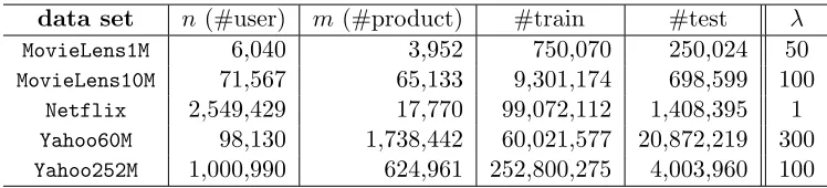
Many machine learning tasks, such as dictionary learning and matrix completion, can be formulated as seeking low rank matrix approximations of a given data matrix. In these problems, one is presented with ann×mmatrixX(perhaps only partially observed) where each column corresponds to a training example and each row corresponds to a feature across examples; the goal is to recover a low rank matrixW that approximates (the observed entries of) X. To achieve this, we assume we are given a convex loss function `(W) :=L(W, X) that measures how wellW approximatesX.2 If we impose a hard bound,t, on the rank of
W, the core training problem can then be expressed as
inf
W:rank(W)≤t `(W) =U∈infRn×tV∈infRt×m `(U V). (43)
Unfortunately, this problem is not convex, and except for special cases (such as SVD) is believed to be intractable.
The two forms of this problem that we will explicitly illustrate in this paper are dictio-nary learning and matrix completion. First, for dictiodictio-nary learning, then×mdata matrix
X is fully observed, then×tmatrixU is interpreted as a “dictionary” consisting oftbasis vectors, and the t×m matrix V is interpreted as the “coefficients” consisting of m code vectors. For this problem, the dictionary and coefficient matrices need to be inferred si-multaneously, in contrast to traditional signal approximation schemes where the dictionary (e.g., the Fourier or a wavelet basis) is fixeda priori. Unfortunately, learning the dictionary with the coefficients creates significant computational challenge since the formulation is no longerjointly convex in the variables U and V, even when the loss`is convex. Indeed, for a fixed dictionary size t, the problem is known to be NP-hard (Vavasis, 2010) except for very special cases (Yu and Schuurmans, 2011).
The second learning problem we illustrate is low rank matrix completion. Here, one observes a small number of entries in X ∈ Rn×m and the task is to infer the remaining entries. In this case, the optimization objective can be expressed as`(W) :=L(P(W−X)), whereL is a reconstruction loss (such as Frobenius norm squared) andP :Rn×m →Rn×m
is a “mask” operator that simply fills the entries corresponding to unobserved indices in
X with zero. Various recommendation problems, such as the Netflix prize,3 can be cast as matrix completion. Due to the ill-posed nature of the problem it is standard to assume that the matrix X can be well approximated by a low rank reconstruction W. Unfortu-nately, the rank function is not convex, hence hard to minimize in general. Conveniently, both the dictionary learning and matrix completion problems are subsumed by the general formulation we consider in (43).
4.2 General Convex Relaxation and Solution via GCG
To develop a convex relaxation of (43), we first consider the factored formulation expressed in terms of U and V on the right hand side. Although it only involves an unconstrained minimization which can be convenient, care is needed to handle the scale invariance intro-duced by the factored form: sinceU can always be scaled andV counter-scaled to preserve
the productU V, some form of penalty or constraint is required to restore well-posedness. A standard strategy is to constrain U, for which a particularly common choice is to constrain its columns to have unit length; i.e.kU:ikc≤1 for alli, whereU:i stands for thei-th column
ofU, andcsimply denotes some norm on the columns. In dictionary learning, for example, this amounts to constraining the basis vectors in the dictionaryU to lie within the unit ball of k·kc. Similar normalization can be used to represent the rows Vi:, with the magnitude
encoded byσi ≥0. In consequence, the unconstrained optimization over`(U V) in (43) can
be reformulated as
min
U∈Rn×t,V∈Rt×m,σ∈Rt `(Udiag(σ)V), s.t. kU:ikc≤1, kVi:kr≤1, and σi≥0. (44)
Here σ := (σ1, σ2, . . . , σt)>, and diag(σ) is a diagonal matrix with the i-th diagonal entry
beingσi. The specific form of the row normk·kr provides additional flexibility in promoting
different structures; for example, the l1 norm leads to sparse solutions, thel2 norm yields
low rank solutions, and block structured norms generate group sparsity. The specific form of the column norm k·kcalso has an effect, as discussed in Section 4.4 below.
Of course the problem remains non-convex. However, it has recently been observed that a simple relaxation of the rank constraint in (43) allows a convex reformulation to be achieved (Argyriou et al., 2008; Bach et al., 2008; Bradley and Bagnell, 2009; Zhang et al., 2011). Observe that replacing the rank constraint with a regularization penalty on the magnitudeσi of each basis pair (U:i, Vi:) yields a relaxed form of (43):
inf
U:kU:ikc≤1
inf
V:kVi:kr≤1
inf
σ:σi≥0
`(Udiag(σ)V) +λkσk1, (45) where the number of columns in U (and also the number of rows in V) is not restricted. Similar to Lasso, thel1 norm on the “singular values” (combination weights)σis used as a
penalty that serves as a convex proxy for rank. By the shrinkage effect of thel1norm, many σi will become zero, implying that the corresponding columns ofU (and rows ofV) can be
dropped. As a result, the rank of the solution—which is indeed unknowna priori—can be chosen adaptively with the trade-off parameter λ≥0.
Importantly, although the problem (45) is still not jointly convex in the factors U, V
and σ, it can be exactly reformulated as a convex optimization as long as `is convex:
(45) = min
W `(W) +λ inf (
X
i
σi :σ≥0, W = X
i
σiU:iVi:,kU:ikc≤1,kVi:kr≤1 )
(46)
= min
W `(W) +λ κ(W), (47)
where the gauge κ is defined by the following setA with uncountably many elements
A:={uv>:u∈Rn,v∈Rm,kukc≤1,kvkr≤1}. (48)
outlined in Section 3.2, yielding an efficient solution method with no additional effort. The reformulation (47) reveals that the relaxed learning problem (45) is essentially considering a rank-one decomposition ofW, which generalizes the singular value decomposition. Further-more it provides a clearer understanding of the computational properties of the regularizer in (47) via its polar:
κ◦(G) = sup
A∈A h
A, Gi= sup
kukc≤1,kvkr≤1
u>Gv (49)
= sup
kvkr≤1
kGvk◦c = sup
kukc≤1
G
> u
◦
r. (50)
Recall that for gauge regularized problems in the form (47), Algorithm 2 only requires approximate computation of the polar (30) in Line 3; hence an efficient method for (ap-proximately) solving (49) immediately yields an efficient implementation. However, this simplicity must be countered by the fact that the polar is not always tractable, since it in-volvesmaximizing a norm subject to a different norm constraint.4 Nevertheless, there exist important cases where the polar can be efficiently evaluated, which we illustrate below.
The polar also allows one to gain insight into the structure of the original gauge regu-larizer, since by duality κ = (κ◦)◦ yields an explicit formula for κ. For example, consider the important special case wherek·kr =k·kc=k·k2. In this case, using (49) one can infer that the polar κ◦(·) = k·ksp is the spectral norm, and therefore the corresponding gauge regularizer κ(·) = k·ktr is the trace norm. In this way, the trace norm regularizer, which
is known to provide a convex relaxation of the matrix rank (Chandrasekaran et al., 2012), can be viewed from the perspective of dictionary learning as an induced norm that arises from a simple 2-norm constraint on the magnitude of the dictionary entriesU:i and a simple
2-norm penalty on the magnitudes of the code vectorsVi:.
This convex relaxation strategy based on convex gauges is quite flexible and has been recently studied for some structured sparse problems (Chandrasekaran et al., 2012; Tewari et al., 2011; Zhang et al., 2012; Bach, 2013). Importantly, the generality of the column and row norms in (45) proffer considerable flexibility to finely characterize the structures sought by low rank learning methods. We will exploit this flexibility in Section 4.4 below to achieve a novel extension of this framework to multi-view dictionary learning (White et al., 2012).
4.2.1 Application to Matrix Completion
We end this subsection with a brief illustration of how the framework can be applied to matrix completion. Recall that in this case one is given a partially observed data matrixX, and the goal is to find a low rank approximatorW that minimizes the reconstruction error on observed entries. In particular, consider the following standard specialization of (47):
min
W∈Rn×m
1
2kPk0 kP(X−W)k
2
F+λkWktr, (51)
where, as noted above,P :Rn×m →Rn×m is the mask operator that fills entries where X
Recht (2009) have proved that, assuming X is (approximately) low-rank, the solution of the convex relaxation (51) will recover the true matrixX with high probability, even when only a smallrandom portion ofX is observed.
Note that, since (51) is a specialization of (47), the modified GCG algorithm, Algo-rithm 2, can be immediately applied. Interestingly, such an approach contrasts with the most popular algorithm favored in the current literature: PG (or its accelerated variant APG; cf. Section 2). The two strategies, GCG versus PG, exhibit an interesting trade-off. Each iteration of PG (or APG) involves solving the PU (9), which in this case requires afull
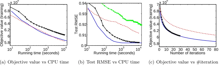
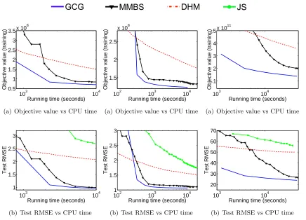
singular value decomposition (SVD) of the current approximant W. The modified GCG method, Algorithm 2, by contrast, only requires the polar of the gradient matrix ∇`(W) to be (approximately) computed in each iteration (i.e. dual of the trace norm; namely, the spectral norm), which is an order of magnitude cheaper to evaluate than a full SVD (cubic versus squared worst case time).5 On the other hand, GCG has a slower theoretical rate than APG,O(1/t) versusO(1/t2), in terms of the number of iterations required to achieve a given accuracy. Once the enhancements in the next section have been incorporated, our experiments in Section 5.1 will demonstrate that GCG is far more efficient than APG for solving the matrix completion problem (51) to tolerances used in practice.
Given the specific objective (51), we may derive a concrete bound onLF used in
Theo-rem 9. Obviously, the smoothness constant is L = 1/kPk0. Suppose we use Monotone
with W0 = 0. So all Wt (and the optimal W) need to satisfy λkWtktr ≤ C, where C=kPXk2F/(2kPk0). Due to the normalization,Ccan be considered a universal constant.
All matricesA∈ Ain (48) satisfy kAkF≤1. Obviously n1kWtk2tr ≤ kWtk2F ≤ kWtk2tr. So
LF ≤2Lsup t
ρ2 α2kAtk
2
F+kWtk 2 F
≤2Lsup
t
ρ2
α2 +kWtk 2 tr
≤ 2
kPk0
1
α2 + 1
C2 λ2. (52)
Ifλneeds to be less than kPk1
0, then the upper bound onLF will beO(kPk0). Notice that under Monotone, the expression of LF in Theorem 5 is on par with the condition number LfD2∗ in (Harchaoui et al., 2015, Theorem 3).
4.3 Fixed-rank Local Optimization
Although the modified GCG algorithm, Algorithm 2, can be readily applied to the refor-mulated low rank learning problem (47), the sublinear rate of convergence established in Theorem 9 is still too slow in practice. Nevertheless, an effective local improvement scheme can be developed that satisfies the properties of a Relaxed subroutine in Algorithm 2, which allows empirical convergence to be greatly accelerated. Recall that in Algorithm 2, the intermediate iterate ˜Wt+1 is determined by a linear combination of the previous
iter-ate Wt and the newly added atom At (we changed the notation from ˜wt+1 to ˜Wt+1 since 5. The per-iteration cost of computing the spectral norm can be further reduced for the sparse matrices occuring naturally in matrix completion, since the gradient matrix in (51) contains at mostk nonzero elements forkequal to the number of observed entries inX. In such cases, anaccurate estimate of the squared spectral norm can be obtained inOklog(√n+m)
the optimization variables are now matrices). We will next demonstrate that ˜Wt+1 can be
further improved by solving a reformulated local problem, and then show how this can still preserve the convergence guarantees of Algorithm 2.
The key reformulation relies on the following fact.
Proposition 15 The convex gauge κ induced by the set A in (48) can be re-expressed as
κ(W) = min
( t X
i=1
kU:ikc kVi:kr:U V =W )
= min
(
1 2
t X
i=1
kU:ik2c+kVi:k2r
:U V =W )
,
for U ∈Rn×t and V ∈Rt×m, as long as t≥mn.
In Appendix B.1 we provide a direct proof that allows us to bound the number of terms involved in the summation. The above lower bound mn ont may not be sharp. For example, if k·kr = k·kc = k·k2, then κ is the trace norm, where
Pt
i=1(kU:ik 2
c+kVi:k 2 r) is
simplykUk2F+kVk2F, the sum of the squared Frobenius norms; that is, Proposition 15 yields the well-known variational form of the trace norm in this case (Srebro et al., 2005). Observe that t in this case can be as low as the rank of W. Theorem 15 also appeared in (Bach et al., 2008; Bach, 2013), although without the explicit boundt≥mn.
Based on Theorem 15, the objective in (47) can then be approximated at iteration tas
Ft+1(U, V) :=`(U V) + λ
2
t+1 X
i=1
kU:ik2c+kVi:k2r
. (53)
Our key intuition is to first factorize ˜Wt+1 into UinitVinit, and then find improvement to
(U, V) with respect to Ft+1 (not the original F). This results inUt+1 and Vt+1 satisfying
Ft+1(Ut+1, Vt+1)≤ Ft+1(Uinit, Vinit). Finally we restore the iterates based on Theorem 15
Wt+1=Ut+1Vt+1 and ρt+1 =
1 2
t+1 X
i=1
k(Ut+1):ik2c+k(Vt+1)i:k2r
. (54)
UsingFt+1 as a surrogate objective for local improvement is particularly advantageous
in computation, because the problem is now unconstrained and the gauge function has been replaced by much simpler forms such askU:ik2c andkVi:k2r. This allows efficient
uncon-strained minimization routines (e.g. L-BFGS) to be applied directly, improving the quality of the current iterate without increasing the size of the dictionary. Note however that (53) is not jointly convex in (U, V) since the size t+ 1 (the iteration counter) is fixed. When
t is sufficiently large, any local minimizer of (53) globally solves the original problem (47) (Burer and Monteiro, 2005)6, but we locally reduce (53) in each iteration even for small t. Once this modification is added to Algorithm 2 we obtain the final variant, Algorithm 3. In this algorithm, Line 3 remains equivalent to before, and Line 4 adopts the slightly more sophisticated update rule in (40), although one can also use (34) with ηt = t+22 . Lines 5
to 8collectively implement theImprovesubroutine: Line 5 splits the iterate into two parts
Algorithm 3 GCG variant for low rank learning. Require: The atomic set A.
1: Initialize W0 =0, ρ0= 0, U0 =V0 = Λ0=∅. 2: fort= 0,1, . . . do
3: (ut,vt)←arg min
uv>∈A
∇`(Wt),uv>
4: (ηt, θt)←arg min
0≤η≤1,θ≥0 `((1−η)Wt+θutv
>
t) +λ((1−η)ρt+θ)
5: Uinit ←(√1−ηtUt,√θtut), Vinit ←(√1−ηtVt>, √
θtvt)>
6: (Ut+1, Vt+1)←Reduce(Ft+1, Uinit, Vinit) s.t. Ft+1(Ut+1, Vt+1)≤ Ft+1(Uinit, Vinit)
e.g. find a local minimum of Ft+1 withU and V initialized toUinit and Vinit resp. 7: Wt+1 ←Ut+1Vt+1 . Nominal as we only maintain (Ut, Vt) in practice 8: ρt+1 ← 12Pit+1=1(k(Ut+1):ik2c+k(Vt+1)i:k2r)
9: end for
Uinit and Vinit, while Line 6 further reduces the reformulated local objective (53) with the
designated initialization (e.g. by finding a local minimum). We referred to it as Reducein order to be distinct fromImprove. The last two steps restore the GCG iterate by (54).
The only major challenge left for inserting a local optimization step in Algorithm 2 is that the Relaxed condition (36) in Theorem 7 must be maintained. This is the condition under which Algorithm 3 retains theO(1/t) rate of convergence established in Theorem 9. Fortunately this holds true as stated in Theorem 16 and its proof is given in Appendix B.2.
Proposition 16 (Uinit, Vinit)in Line 5 is a factorization of the intermediate iterateW˜t+1=
(1−ηt)Wt+θtutv>t . Let(Ut+1, Vt+1) improve upon it in the sense that Ft+1(Ut+1, Vt+1)≤
Ft+1(Uinit, Vinit). Then the Wt+1 and ρt+1 recovered by (54) satisfy theRelaxed condition.
Although the Reduce subroutine is not guaranteed to achieve strict improvement in every iteration, we observe in our experiments in Section 5 below that Algorithm 3 is almost always significantly faster than the Null version of Algorithm 2. In other words, local acceleration appears to make a big difference in practice.
Remark 17 Interleaving local improvement with a globally convergent procedure has been considered by Mishra et al. (2013) and Laue (2012). In particular, Laue (2012) considered the constrained problem (21), which unfortunately leads to considering a constrained min-imization for local improvement that can be less efficient than the unconstrained approach considered in (53). In addition, Laue (2012) used the original objective F directly in local optimization. This leads to significant challenge when the regularizer κ is complicated such as the trace norm, and we avoid this issue by using a smooth surrogate objective Ft+1.
Focusing on trace norm regularization only, Mishra et al. (2013) proposed a trust-region procedure that locally minimizes the originalobjective on the Stiefel manifold and the positive semidefinite cone, which unfortunately also requires constrained minimization and dynamic maintenance of the singular value decomposition of a small matrix. The rate of convergence of this procedure has not been analyzed.
considered by the standard fixed rank approach to matrix factorization, the overall perfor-mance of Algorithm 3 can be substantially improved by leveraging the techniques that have been developed for this specific objective. These improvements include system level opti-mizations such as stochastic solvers on distributed, parallel and asynchronous infrastruc-tures (Zhuang et al., 2013; Yun et al., 2014). In the experiments conducted in Section 5 below, we merely solve (54) using a generic L-BFGS solver to highlight the efficiency of the GCG framework itself. Nevertheless, such a study leaves significant room for further straightforward acceleration.
Remark 19 Much of our development in this section was inspired by the work of Bach et al. (2008), who first demonstrated, although in a slightly less clear way, that the convex relaxation in (47)is possible, but did not observe the computational connection to GCG. Our contribution here is to present this result succinctly using the notion of convex gauges, con-nect it naturally to the GCG algorithm we developed in Section 3, and propose an efficient fixed-rank local improvement subroutine Reducethat does not affect theoretical convergence guarantees. After our conference version (Zhang et al., 2012), Bach (2013) also indepen-dently extended the previous work (Bach et al., 2008) using convex gauges, and discussed a multiplicative approximate GCG variant similar to our Algorithm 2. However, the pos-sibility to intervene fixed-rank local subroutines based on Theorem 15 with GCG, and its practical computational consequences, were not observed in (Bach, 2013).
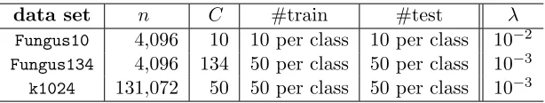
4.4 Multi-view Dictionary Learning
Finally, in this section we show how low rank learning can be generalized to a multi-view setting where, once again, the modified GCG algorithm can efficiently provide optimal solutions. The key challenge in this case is to develop column and row norms that can capture the more complex problem structure.
Consider a two-view learning task where one is given m paired observations
nhxj
yj
io
consisting of an x-view and a y-view with lengths n1 and n2 respectively. The goal is to
infer a set of latent representations, hj (of dimension t <min(n1, n2)), and reconstruction
models parameterized by the matrices A and B, such that Ahj ≈ xj and Bhj ≈ yj for
all j. In particular, let X denote then1×m matrix of x-view observations,Y then2×m
matrix ofy-view observations, and Z =
h X Y i
the concatenated (n1+n2)×m matrix. The problem can then be expressed as recovering an (n1+n2)×tmatrix of model parameters, C=
h A B i
, and at×m matrix of latent representations, H, such thatZ ≈CH.
The key assumption behind multi-view learning is that each of the two views,xj andyj,
is conditionally independent given the shared latent representation, hj. Although
multi-view data can always be concatenated hence treated as a single multi-view, explicitly representing multiple views enables more accurate identification of the latent representation (as we will see), when the conditional independence assumption holds. To better motivate this model, it is enlightening to first reinterpret the classical formulation of multi-view dictionary learn-ing, which is given by canonical correlation analysis (CCA). Typically, it is expressed as the problem of projecting two views so that the correlation between them is maximized. Assuming the data is centered (i.e. X1 = 0 and Y1 = 0), the sample covariance of X
optimization over matrix variables
max
U,V tr(U
>XY>V) s.t. U>XX>U =V>Y Y>V =I (55)
forU ∈Rn1×t, V ∈Rn2×t (De Bie et al., 2005). HereI is the identity matrix whose size is clear from the context. Although this classical formulation (55) does not make the shared latent representation explicit, CCA can be expressed by a generative model: given a latent representation, hj, the observationsxj =Ahj+j and yj =Bhj+νj are generated by a
linear mapping plus independent zero mean Gaussian noise, ∼ N(0,Σx), ν ∼ N(0,Σy)
(Bach and Jordan, 2006). Interestingly, one can show that the classical CCA problem (55) is equivalent to the following multi-view dictionary learning problem.
Proposition 20 (White et al. 2012, Proposition 1) Fix t, let
(A, B, H) = arg min
A:kA:ik2≤1 min
B:kB:ik2≤1 min H
(XX>)−1/2X
(Y Y>)−1/2Y − A B H 2 F . (56)
Then U= (XX>)−21A and V= (Y Y>)− 1
2B provide an optimal solution to (55).
Proposition 20 demonstrates how formulation (56) respects the conditional independence of the separate views: given a latent representationhj, the reconstruction losses on the two
views, xj and yj, cannot influence each other, since the reconstruction models A and B
are individually constrained. By contrast, in single-view dictionary learning (i.e. principal component analysis) A and B are concatenated in the larger variable C =
h A B i
, where C
as a whole is constrained butA and B are not. A and B must then compete against each other to acquire magnitude to explain their respective “views” given hj (i.e. conditional
independence is not enforced). Such sharing can be detrimental if the two views really are conditionally independent givenhj.
This matrix factorization viewpoint has recently allowed dictionary learning to be ex-tended from the single-view setting to the multi-view setting (Jia et al., 2010). However, despite its elegance, the computational tractability of CCA hinges on its restriction to squared loss under a particular normalization, precluding other important losses. To com-bat these limitations, we apply the same convex relaxation principle as in Section 4.2. In particular, we reformulate (56) by first incorporating an arbitrary loss function ` that is convex in its first argument, and then relaxing the rank constraint by replacing it with thel1 norm of the “singular values”. This amounts to the following training problem that
extends (Jia et al., 2010):
min
A,B,H,σ`
A B
diag(σ)H;Z
+λkσk1, s.t. kHi:k2≤1, σi ≥0,
A:i B:i
∈ D ∀i,
where D:=
a b
:kak2 ≤β, kbk2 ≤γ
. (57)