Smoothing Multivariate Performance Measures

Smoothing Multivariate Performance Measures

Xinhua Zhang∗ [email protected]

Department of Computing Science University of Alberta

Alberta Innovates Center for Machine Learning Edmonton, Alberta T6G 2E8, Canada

Ankan Saha [email protected]

Department of Computer Science University of Chicago

Chicago, IL 60637, USA

S.V.N. Vishwanathan [email protected]

Departments of Statistics and Computer Science Purdue University

West Lafayette, IN 47907-2066, USA

Editor:Sathiya Keerthi

Abstract

Optimizing multivariate performance measure is an important task in Machine Learning. Joachims (2005) introduced a Support Vector Method whose underlying optimization problem is commonly

solved by cutting plane methods (CPM_{s) such as}SVM-Perf_andBMRM_{. It can be shown that}CPM_s

converge to anεaccurate solution inO _λε1iterations, whereλis the trade-off parameter between

the regularizer and the loss function. Motivated by the impressive convergence rate ofCPM_on

a number of practical problems, it was conjectured that these rates can be further improved. We disprove this conjecture in this paper by constructing counter examples. However, surprisingly, we further discover that these problems are not inherently hard, and we develop a novel smoothing

strategy, which in conjunction with Nesterov’s accelerated gradient method, can find anε

accu-rate solution inO∗minn1_ε,_√1

λε o

iterations. Computationally, our smoothing technique is also particularly advantageous for optimizing multivariate performance scores such as precision/recall

break-even point andROCArea_{; the cost per iteration remains the same as that of}CPM_s.

Empiri-cal evaluation on some of the largest publicly available data sets shows that our method converges

significantly faster thanCPM_{s without sacrificing generalization ability.}

Keywords: non-smooth optimization, max-margin methods, multivariate performance measures, Support Vector Machines, smoothing

1. Introduction

Recently there has been an explosion of interest in applying machine learning techniques to a num-ber of application domains, much of which has been fueled by the phenomenal success of binary Support Vector Machines (SVMs). At the heart of SVMs is the following regularized risk

mization problem:

min

w J(w) =

λ

2kwk 2

+Remp(w). (1)

HereRemp is the so-called empirical risk (see below), 1₂kwk2 is the regularizer, λ>0 is a scalar which trades off the importance of the empirical risk and the regularizer. Given a training set with

nexamples

X

:=_{(xi,yi)}ni=1wherexi∈Rpandyi∈ {±1}, the empirical riskRempminimized by SVMs is the average of the hinge loss:

Remp(w):= 1

n n

∑

i=1

max(0,1₋yihw,xii), (2)

where_h·,_·idenotes the Euclidean dot product.

Binary SVMs optimize classification accuracy, while many application areas such as Natural Language Processing (NLP) frequently use more involved multivariate performance measures such as precision/recall break-even point (PRBEP_{) and area under the Receiver Operating Characteristic}

curve (ROCArea_{). Joachims (2005) proposed an elegant SVM based formulation for directly}

op-timizing these performance metrics. In his formulation, the empirical riskRempin (1) is replaced by

Remp(w):= max z∈{−1,1}n

"

∆(z,y) +1 n

n

∑

i=1

hw,xii(zi−yi) #

. (3)

Here, ∆(z,y) is the multivariate discrepancy between the correct labels y:= (y1, . . . ,yn)⊤ and a candidate labelingz:= (z1, . . . ,zn)⊤∈ {±1}n. In order to compute the multivariate discrepancy for

PRBEP_{we need the false negative and false positive rates, which are defined as}

b=

_∑

i∈P

δ(zi=−1) and c=

∑

j∈N

δ(zj=1), respectively.

Hereδ(x) =1 ifxis true and 0 otherwise, while

P

and

N

denote the set of indices with positive (yi= +1) and negative (yi=−1) labels respectively. Furthermore, letn+=|

P

|,n−=

N

. With this notation in place,∆(zzz,yyy)forPRBEP_{is defined as}

∆(zzz,yyy) = (

b/n+ ifb=c

−∞ otherwise. (4)

ROCArea_{, on the other hand, measures how many pairs of examples are mis-ordered. Denote}

m=n+n−. Joachims (2005) proposed using the following empirical risk,Remp, to directly optimize

theROCArea_:1

Remp(w) = 1

mz∈{max0,1}m

"

∑

i∈P j

∑

∈N

zi j h

1₋w⊤(xi−xj) i#

. (5)

We will call the regularized risk minimization problem with thePRBEP_{loss (3) as the}PRBEP

-problem and with the ROCArea _{loss (5) as the} ROCArea_{-problem respectively. As is obvious,}

both these problems entail minimizing a non-smooth objective function which isnotadditive over the data points. Fortunately, cutting plane methods (CPM_{s) such as} SVM-Perf _{(Joachims, 2006)}

and BMRM_{(Teo et al., 2010) can be used for this task. At each iteration these algorithms only}

require a sub-gradient ofRemp, which can be efficiently computed by aseparationalgorithm with

O(nlogn)effort for both (3) and (5) (Joachims, 2005). In this paper, we will work withBMRM_as

our prototypicalCPM_{, which, as Teo et al. (2010) point out, includes}SVM-Perf_{as a special case.} CPM_{s are popular in Machine Learning because they come with strong convergence guarantees.}

The tightest upper bound on the convergence speed ofBMRM_{, which we are aware of, is due to Teo}

et al. (2010). Theorem 5 of Teo et al. (2010) asserts thatBMRM_{can find anε-accurate solution of}

the regularized risk minimization problem (1) with non-smooth empirical risk functions such as (3) and (5) after computingO(_λε1)subgradients. This upper bound is built upon the following standard assumption:

Assumption 1 (A1) The subgradient of Remp is bounded, that is, at any point w, there exists a

subgradient ggg∈∂Remp(w)such thatkgggk ≤G<∞.

In practice the observed rate of convergence ofBMRM_{is significantly faster than predicted by}

the-ory. Therefore, it was conjectured that perhaps a more refined analysis might yield a tighter upper bound (Teo et al., 2010). Our first contribution in this paper is to disprove this conjecture under assumptionA1. We carefully constructPRBEP_andROCArea_{problems on which}BMRM_requires

at least Ω(1/ε) iterations to converge for a fixed λ. It is worthwhile emphasizing here that due to the specialized form of the objective function in (1), lower bounds forgeneralconvex function classes such as those studied by Nesterov (2003) and Nemirovski and Yudin (1983) do not apply. In addition, our examples stick to binary classification and are substantially different from the one in Joachims et al. (2009) which requires an increasing number of classes.

This result leads to the following natural question: do the lower bounds hold because thePRBEP

andROCArea_{problems are fundamentally hard, or is it an inherent limitation of} CPM_{? In other}

words, does there exist a solver which solves thePRBEP_andROCArea_{problems by invoking the}

separation algorithm for fewer than O(_λε1) times?2 We provide partial answers. To understand our results one needs to understand another standard assumption that is often made when proving convergence rates:

Assumption 2 (A2) Eachxilies inside an L2(Euclidean) ball of radius R, that is,kxik ≤R.

Clearly assumption A2is more restrictive than A1, because _kxxxik ≤Rimplies that for all www, any

subgradient of RemphasL2 norm at most 2R in both (3) and (5). Our second contribution in this paper is to show that theO(_λε1)barrier can be broken under assumptionA2, while making a similar claim just under assumptionA1remains an open problem. In a nutshell, our algorithm approximates (1) by a smooth function, which in turn can be efficiently minimized by using either accelerated gradient descent (Nesterov, 1983, 2005, 2007) or a quasi-Newton method (Nocedal and Wright, 2006). This technique for non-smooth optimization was pioneered by Nesterov (2005). However, applying it to multivariate performance measures requires special care. We now describe some relevant details and point out technical difficulties that one encounters along the way.

1.1 Nesterov’s Formulation

LetAbe a linear transform and assume that we can find a smooth functiong⋆_µ(A⊤w)with a Lipschitz continuous gradient such thatRemp(w)−g⋆µ(A⊤w)

≤µfor allw. It is easy to see that

Jµ(w):=λ

2kwk 2

+g⋆_µ(A⊤w) (6)

satisfies Jµ(w)−J(w)

≤µ for all w. In particular, if we set µ=ε/2 and find a w′ such that

Jµ(w′)_≤minwJµ(w) +ε/2, then it follows thatJ(w′)_≤minwJ(w) +ε. In other words, w′ is anε

accurate solution for (1).

By applying Nesterov’s accelerated gradient method toJµ(w)one can find anε-accurate solution

of the original nonsmooth problem (1) after querying the gradient ofg⋆_µ(A⊤w)at most

O∗ _√

D_kA_kmin

1

ε,

1 √

λε

(7)

number of times (Nesterov, 1983, 2005).3 Here _kA_k is the matrix norm of A, which is defined as_kA_k=max_uuu,vvv:kuuuk=kvvvk=1uuu⊤Avvv=

p

λmax(A⊤A), withλmax denoting the maximum eigenvalue of

A, when the norm considered is the Euclidean norm. Furthermore, Dis a geometric constant that depends solely ongµand is independent ofε,λ, orA. Compared with theO(_λε1)rates ofCPMs, the

1

√

λε part in (7) is already superior. Furthermore, many applications requireλ≪εand in this case the 1_ε part of the rate is even better. Note thatCPM_{s rely on} λ

2kwk

2_{to stabilize each update, and it} has been empirically observed that they converge slowly whenλis small (see, e.g., Do et al., 2009). Although the above scheme is conceptually simple, the smoothing of the objective function in (1) has to be performed very carefully in order to avoid dependence onn, the size of the training set. The main difficulties are two-fold. First, one needs to obtain a smooth approximationg⋆_µ(A⊤w)to

Remp(w)such that √

D_kA_kis small (ideally a constant). Second, we need to show that computing the gradient ofg⋆_µ(A⊤w) is no harder than computing a subgradient ofRemp(w). In the sequel we will demonstrate how both the above difficulties can be overcome. Before describing our scheme in detail we would like to place our work in context by discussing some relevant related work.

1.2 Related Work

Training large SV models by using variants of stochastic gradient descent has recently become increasingly popular (Bottou, 2008; Shalev-Shwartz et al., 2007). While the dependence onεandλ

is stillΩ(1

λε)or worse (Agarwal et al., 2009), one gets bounds on the computational cost independent ofn. However, stochastic gradient descent can only be applied when the empirical risk isadditively decomposable, that is, it can be written as the average loss over individual data points like in (2). Since the non-linear multivariate scores such as the ones that we consider in this paper are not additively decomposable, this rules out the application of online algorithms to these problems.

Traditionally, batch optimizers such as the popular Sequential Minimal Optimization (SMO) worked in the dual (Platt, 1998). However, as List and Simon (2009) show, for the empirical risk (2) based on hinge loss, if the matrix which contains the dot products of all training instances

(also known as the kernel matrix) is not strictly positive definite, then SMO requiresO(n/ε) iter-ations with each iteration costingO(np)effort. However, when the kernel matrix is strictly posi-tive definite, then one can obtain anO(n2log(1/ε))bound on the number of iterations, which has better dependence on ε, but is prohibitively expensive for large n. Even better dependence onε

can be achieved by using interior point methods (Ferris and Munson, 2002) which require only

O(log(log(1/ε))iterations, but the time complexity per iteration isO(min_{n2p,p2n_}).

Recently, there has been significant research interest in optimizers which directly optimize (1) because there are some distinct advantages (Teo et al., 2010). Chapelle (2007) observed that to find awwhich generalizes well, one only needs to solve the primal problem to very low accuracy (e.g., ε_≈0.001). In fact, to the best of our knowledge, Chapelle (2007) introduced the idea of smoothing the objective function to the Machine Learning community. Specifically, he proposed to approximate the binary hinge loss by a smooth Huber’s loss and used the Newton’s method to solve this smoothed problem. This approach yielded the best overall performance in the Wild Competition Track of Sonnenburg et al. (2008) for training binary linear SVMs on large data sets. A similar smoothing approach is proposed by Zhou et al. (2010), but it is also only for hinge loss.

However, the smoothing proposed by Chapelle (2007) for the binary hinge loss is rather ad-hoc, and does not easily generalize to (3) and (5). Moreover, a function can be smoothed in many different ways and Chapelle (2007) did not explicitly relate the influence of smoothing on the rates of convergence of the solver. In contrast, we propose principled approaches to overcome these problems.

Of course, other smoothing techniques have also been explored in the literature. A popular approach is to replace the nonsmooth max term by a smooth log-sum-exp approximation (Boyd and Vandenberghe, 2004). In the case of binary classification this approximation is closely related to logistic regression (Bartlett et al., 2006; Zhang, 2004), and is equivalent to using an entropy regularizer in the dual. However, as we discuss in Section 3.1.2 this technique yields exorbitantly large√D_kA_kin the bound (7) when applied to optimize multivariate performance measures.

1.3 Notation And Paper Outline

We assume a standard setup as in Nesterov (2005). Lower bold case letters (e.g., w, µµµ) denote vectors,wi denotes thei-th component ofw,0 refers to the vector with all zero components,eeei is

thei-th coordinate vector (all 0’s except 1 at thei-th coordinate) and∆krefers to thekdimensional

simplex. Unless specified otherwise,_k·krefers to the Euclidean norm_kw_k:=p_hwww,www_i. We denote

R:=R∪ {∞_}, and[t]:=_{1, . . . ,t_}.g⋆stands for the Fenchel dual of a functiong, and∂g(www)is the subdifferential ofgatwww(the set of all subgradients ofgatwww).

In Section 2, we first establish the lower bounds on the rates of convergence of CPM_{s when}

used to optimize the regularized risk of PRBEP _and ROCArea_{. To break this lower bound, our}

1.4 Improvement On Earlier Versions Of This Paper

This paper is based on two prior publications of the same authors: Zhang et al. (2011a) at NIPS 2010 and Zhang et al. (2011b) at UAI 2011, together with a technical report (Zhang et al., 2010). Major improvements have been made on them, which include:

• New lower bounds forPRBEP_andROCArea_{losses (see Sections 2.2 and 2.3 respectively).}

• Significantly simplified algorithms for computing the gradient of smoothed objectives for

bothPRBEP_andROCArea_{losses (See Sections 4.1 and 4.2 respectively).}

• Empirical evaluation on some of the largest publicly available data sets including those from the Pascal Large Scale Learning Workshop in Section 5 (Sonnenburg et al., 2008)

• Open source code based on PETSc (Balay et al., 2011) and TAO (Benson et al., 2010) pack-ages made available for download from Zhang et al. (2012).

2. Lower Bounds For Cutting Plane Methods

BMRM_{(Teo et al., 2010) is a state-of-the-art cutting plane method for optimizing multivariate}

per-formance scores which directly minimizes the non-smooth objective functionJ(www). At every itera-tion,BMRM_{replacesRempby a piecewise linear lower boundR}cp

k and obtains the next iteratewk by

optimizing

wk:=argmin w w w

Jk(w):= λ

2kwk 2_+Rcp

k (w), where R

cp

k (w):=max

i∈[k]hw,aii+bi. (8)

Here ai∈∂Remp(wi₋1) denotes an arbitrarysubgradient ofRemp at wi₋1 andbi =Remp(wi₋1)− hwi−1,aii. The piecewise linear lower bound is successively tightened until the gap

εk:= min

0≤t≤kJ(wt)−Jk(wk) (9)

falls below a predefined toleranceε.

SinceJkin (8) is a convex objective function, the optimalwwwkcan be obtained by solving its dual

problem, which is a quadratic programming problem with simplex constraints. We refer the reader to Teo et al. (2010) for more details. The overall procedure ofBMRM_{is summarized in Algorithm}

1. Under AssumptionA1, Teo et al. (2010) showed thatBMRM_{converges atO(}1

λε)rates:

Theorem 3 Suppose Assumption 1 holds. Then for anyε<4G2/λ,BMRM_{converges to anε}

accu-rate solution of (1)as measured by(9)after at most the following number of steps:

log₂λJ(0)

G2 + 8G2

λε −1.

2.1 Lower Bound Preliminaries

Algorithm 1:BMRM_.

Input: A tolerance level of function valueε.

1 Initialize:www0to arbitrary value, for example,0. Letk=1.

2 while TRUE do

3 Pick arbitrary subgradient ofRempatwk−1:ak∈∂Remp(wk−1). 4 Letb_k=Remp(wk−1)− hwk−1,aki.

5 Solvew_k=argmin_wJ_k(w) =argmin_w

n λ 2kwk

2_+max

i∈[k]{hw,aii+bi} o

.

6 ifmin0_≤t≤kJ(wt)−Jk(wk)<εthen returnwwwk. elsek=k+1.

minimizing the objective functionJ(w)defined in (1), if we minimize a scaled versioncJ(w)this scales the approximation gap (9) byc. AssumptionA1fixes this degree of freedom by bounding the scale of the objective function.

Given a function f_∈

F

and an optimization algorithmA, suppose_{wk}are the iterates produced

by some algorithmAwhen minimizing some function f. DefineT(ε;f,A)as the first step indexk

whenwk becomes anεaccurate solution:4

T(ε;f,A) =min_{k: f(wk)−minwwwf(www)≤ε}.

Upper and lower bounds are both properties for a pair of

F

andA. A functionκ(ε) is called an

upper bound of(

F

,A)if for all functions f _∈

F

and allε>0, it takesat mostorderκ(ε)steps for

Ato reduce the gap to less thanε, that is,

(UB) _∀ε>0,_∀ f _∈

F

,T(ε;f,A)_≤κ(ε).

On the other hand, we define lower bounds as follows. κ(ε)is calledalower bound of(

F

,A)if for anyε>0, there exists a function fε∈

F

depending onε, such that it takesat leastκ(ε)steps forA to find anεaccurate solution of fε:

(LB) _∀ε>0,_∃ fε∈

F

,s.t. T(ε;fε,A)≥κ(ε).

Clearly, this lower bound is sufficient to refute upper bounds or to establish their tightness. The size of the function class

F

affects the upper and lower bounds in opposite ways. Suppose

F

′_⊂

F

. Proving upper (resp. lower) bounds on (

F

′_{,A)is usually easier (resp. harder) than proving upper}

(resp. lower) bounds for(

F

,A). Since the lower bounds studied by Nesterov (2003) and Nemirovski and Yudin (1983) are constructed by usinggeneralconvex functions, they do not apply here to our specialized regularized risk objectives.

We are interested in bounding theprimal gapof the iterateswk:J(wk)−minwwwJ(www). Data sets

will be constructed explicitly whose resulting objectiveJ(w)will be shown to satisfy Assumption

A1and attain the lower bound ofBMRM_{. We will focus on theRempfor both the}PRBEP_{loss in (3)}

and theROCArea_{loss in (5).}

4. The initial point also matters, as in the best case one can just start from the optimal solution. Thus the quantity of interest is actuallyT(ε;f,A):=maxw0min{k:f(wk)−minwwwf(www)≤ε, starting point beingw0}. However, without

2.2 Construction Of Lower Bound ForPRBEP_Problem

Given ε>0, let n=_⌈1/ε_⌉+1 and construct a data set _{(xxxi,yi)}ni=1 as follows. Setc=

√

2 4 , and let eeei denote the i-th coordinate vector in Rn+2 (p=n+2). Let the first example be the only

positive example: y1= +1 andxxx1=cneee2. The restn−1 examples are all negative: yi=−1 and xxxi=−cneee3−cneeei+2fori∈[2,n]. This data set concretizes theRempin (3) as follows:

Remp(www) = max

zzz∈{−1,1}n

"

∆(zzz,yyy) +1

nhwww,xxx1i(z1−1) +

1

n n

∑

i=2

hwww,xxxii(zi+1)

| {z }

:=ϒ(zzz)

#

.

Setting λ=1, we obtain the overall objective J(www)in (1). Now we have the following lower bound on the rates of convergence ofBMRM_.

Theorem 4 Let www0=eee1+2ceee2+2ceee3. Suppose runningBMRMon the above constructed objective

J(www)produces iteratesw1, . . . ,wk, . . .. Then it takesBMRMat least ₁

5ε

steps to find anεaccurate solution. Formally,

min

i∈[k]J(wi)−minwww J(www)≥

1 4

1

k−

1

n₋1

for allk_∈[n₋1],

hence min

i∈[k]J(wi)−minwww J(www)>εfor allk<

1 5ε.

Proof The crux of our proof is to show

wwwk=2ceee2+2ceee3+ 2c

k k+3

∑

i=4

eeei, for allk∈[n−1]. (10)

We prove it by induction. Initially atk=1, we note

1

nhwww0,xxx1i=2c

2₌1 4, and

1

nhwww0,xxxii=−2c

2₌

−1₄, _∀i_∈[2,n]. (11)

Since there is only one positive example,zzzcan only have two cases. Ifzzz=yyy(i.e., correct labeling withb=0), thenϒ(zzz) =ϒ(yyy) =0. Ifzzzmisclassifies the only positive example into negative (i.e.,

b=1), then∆(zzz,yyy) =_nb₊ =1. SincePRBEP_{forcesc=b=1, there must be one negative example}

misclassified into positive by zzz. By (11), all i∈[2,n]play the same role in ϒ(zzz). Without loss of generality, assume the misclassified negative example isi=2, that is, zzz= (₋1,1,₋1,₋1, . . .). It is easy to check thatϒ(zzz) =1+2

n[−hwww0,xxx1i+hwww0,xxx2i] =0=ϒ(yyy), which means suchzzzis a

maximizer ofϒ(zzz). Using thiszzz, we can derive a subgradient ofRemp(www0):

a aa1=

2

n(−xxx1+xxx2) =−2ceee2−2ceee3−2ceee4andb1=0− haaa1,www0i=4c

2_+4c2_=1,

www1=argmin

www

1 2kwwwk

2₊

haaa1,wwwi+b1

=2ceee2+2ceee3+2ceee4.

Next assume (10) holds for steps 1, . . . ,k(k_∈[n₋2]). Then at stepk+1 we have

1

nhwwwk,xxx1i=2c

2₌ 1 4, and

1

nhwwwk,xxxii= (

−2c2₋2_kc2 =₋1 4−

1

Again consider two cases ofzzz. If zzz=yyythenϒ(zzz) =ϒ(yyy) =0. Ifzzzmisclassifies the only positive example into negative, then∆(zzz,yyy) =1. Ifzzz misclassifies any ofi_∈[2,k+1]into positive, then

ϒ(zzz) =1+2

n[−hwwwk,xxx1i+hwwwk,xxxii] =−

1

2k <ϒ(yyy). So suchzzzcannot be a maximizer ofϒ(zzz). But

ifzzzmisclassifies any ofi≥k+2 into positive, thenϒ(zzz) =1+2

n[−hwwwk,xxx1i+hwwwk,xxxii] =0=ϒ(yyy).

So suchzzzis a maximizer. Picki=k+2 and we can derive from thiszzza subgradient ofRemp(wwwk):

a a ak+1=

2

n(−xxx1+xxxk+2) =−2ceee2−2ceee3−2ceeek+4, bk+1=0− haaak+1,wwwki=4c

2_+4c2_=1,

w

wwk+1=argmin

w w w

Jk+1(www) =argmin

w w w

1 2kwwwk

2

+max

i∈[k+1]{haaai,wwwi+bi}

=2ceee2+2ceee3+ 2c k+1

k+4

∑

i=4

eeei.

To verify the last step, note_haaai,wwwk+1i+bi=_2(k+−1₁₎for alli∈[k+1], and so∂Jk+1(wwwk+1) ={wwwk+1+

∑k+_i=11αiaaai:ααα∈∆k+1} ∋0(just set allαi=_k+1₁). So (10) holds for stepk+1. (End of induction.)

All that remains is to observeJ(wwwk) =1₄(2+1_k)while minwwwJ(www)≤J(wwwn−1) =1₄(2+_n−1₁), from which it follows thatJ(wwwk)₋minwwwJ(www)≥1₄(1_k−_n−1₁).

Note in the above run ofBMRM_{, all subgradientsaaak have norm}

q

3

2 which satisfies Assumption 1.

2.3 Construction Of Lower Bound ForROCArea_Problem

Next we consider the case ofROCArea_{. Givenε>0, define n=⌊1/ε⌋and construct a data set}

{(xxxi,yi)}n+i=11withn+1 examples as follows. Leteeeibe thei-th coordinate vector inRn+2(p=n+2).

The first example is the only positive example withy1= +1 andxxx1=√neee2. The restnexamples are all negative, withyi=−1 andxxxi=−neeei+1fori∈[2,n+1]. Then the corresponding empirical risk forROCArea_{loss is}

Remp(www) = 1

n n+1

∑

i=2

max_{0,1_{− h}www,xxx1−xxxii}=

1

n n+1

∑

i=2

max_{0,1_{− h}www,√neee2+neeei+1

| {z }

:=uuui

i}.

By further setting λ=1, we obtain the overall objective J(www) in (1). It is easy to see that

the minimizer ofJ(www) isw∗= 1₂√1_neee2+1_n∑n+_i=32eeei

andJ(w∗) = ₄1_n. In fact, simply check that hw∗,uuuii=1 for alli, so∂J(w∗) =

n

w∗₋∑ni=1αi

1

√_neee2+eeei+2

:αi∈[0,1] o

, and setting allαi=₂1_n

yields the subgradient0. Then we have the following lower bound on the rates of convergence for

BMRM_.

Theorem 5 Letw0=eee1+√1_neee2. Suppose runningBMRMon the above constructed objective J(www)

produces iterates w1, . . . ,wk, . . .. Then it takes BMRM at least ₂

3ε

steps to find an ε accurate solution. Formally,

min

i∈[k]J(wi)−J(w ∗_{) =} 1

2k+

1

4n for allk∈[n],hence mini∈[k]J(wi)−J(w

∗_{)>εfor allk<} 2

3ε.

Proof The crux of the proof is to show that

w w wk=

1 √

neee2+

1

k k+2

∑

i=3

We prove (12) by induction. Initially atk=1, we note that_hwww0,uuuii=1 for alli∈[2,n+1]. Hence

we can derive a subgradient andwww1:

a aa1=−

1

nuuu2=−

1 √

neee2−eee3, b1=−haaa1,www0i=

1

n,

w

ww1=argmin

w ww

1 2kwwwk

2

+_haaa1,wwwi+b1

=₋aaa1= 1 √

neee2+eee3.

So (12) holds fork=1. Now suppose it hold for steps 1, . . . ,k(k_∈[n₋1]). Then for stepk+1 we note

hwwwk,uuuii= (

1+n_k ifi_≤k

1 ifi_≥k+1.

Therefore we can derive a subgradient and computewwwk+1:

a

aak+1=− 1

nuuuk+2=−

1 √

neee2−eeek+3, bk+1=−haaak+1,wwwki=

1

n,

wwwk+1=argmin

w ww

n₁

2kwwwk

2_{+ max}

i∈[k+1]{haaai,wwwi+bi}

| {z }

:=Jk+1(www)

o

=₋ 1 k+1

k+1

∑

i=1

a aai=

1 √_neee2+

1

k+1

k+3

∑

i=3

eeei.

This minimizer can be verified by noting that _hwwwk+1,aaaii+bi=−_k+1₁ for all i∈[k+1], and so ∂Jk+1(wwwk+1) ={wwwk+1+∑k+i=11αiaaai:ααα∈∆k+1} ∋0 (just set allαi= _k+1₁). So (12) holds for step k+1. (End of induction.)

All that remains is to observeJ(wwwk) =₂1(1_n+1_k).

As before, in the above run of BMRM_{, all subgradients aaak have norm (1+}1

n)

1/2 _{which satisfies} Assumption 1.

3. Reformulating The Empirical Risk

In order to bypass the lower bound of CPM_{s and show that the multivariate score problems can}

be optimized at faster rates, we propose a smoothing strategy as described in Section 1.1. In this section, we will focus on the design of smooth surrogate functions, with emphasis on the consequent rates of convergence when optimized by Nesterov’s accelerated gradient methods (Nesterov, 2005). The computational issues will be tackled in Section 4.

In order to approximate Remp by g⋆µ we will start by writing Remp(w) asg∗(A⊤w) for an ap-propriate linear transformAand convex functiong. Let the domain ofgbeQandd be a strongly convex function with modulus 1 defined onQ. Furthermore, assume minααα∈Qd(ααα) =0 and denote D=maxααα∈Qd(ααα). In optimization parlancedis called aprox-function. Set

g⋆_µ= (g+µd)⋆.

Then by the analysis in Appendix A, we can conclude that g⋆_µ(A⊤w) has a Lipschitz continuous gradient with constant at most 1_µkA_k2. In addition,

g⋆µ(A⊤w)−Remp(w)

Choosingµ=ε/D, we can guarantee the approximation is uniformly upper bounded byε.

There are indeed many different ways of expressing Remp(w) as g⋆(A⊤w), but the next two sections will demonstrate the advantage of our design.

3.1 Contingency Table Based Loss

Letting

S

k_{denote thekdimensional probability simplex, we can rewrite (3) as:}

Remp(w) = max

zzz∈{−1,1}n "

∆(zzz,yyy) +1 n

n

∑

i=1

hw,xxxii(zi−yi) #

(14)

= max α

αα∈S2n

∑

zzz∈{−1,1}n

αzzz ∆(zzz,yyy) +

1

n n

∑

i=1

hw,xxxii(zi−yi) !

(15)

= max α

αα∈S2n

∑

zzz∈{−1,1}n

αzzz∆(zzz,yyy)−

2

n n

∑

i=1

yihw,xxxii

∑

zzz:zi=−yi

αzzz !

.

Note from (14) to (15), we defined 0_·(₋∞) =0 since ∆(zzz,yyy) can be ₋∞as in (4). Introduce

βi=∑zzz:zi=−yiαzzz. Thenβi∈[0,1]and one can rewrite the above equation in terms ofβββ:

Remp(w) = max β β β∈[0,1]n

( −2

n n

∑

i=1

yihw,xxxiiβi−g(βββ) )

(16)

where g(βββ):=₋ max α α

α∈A(βββ)_zzz

∑

∈{−1,1}n

αzzz∆(zzz,yyy). (17)

Here

A

(βββ) is a subset of

S

2n

defined via

A

(βββ) =αααs.t. ∑zzz:zi=−yiαzzz=βi for alli . Indeed, this rewriting only requires that the mapping fromααα_∈

S

2n _{toβββ∈Q:= [0,1]}n_{is surjective. This is clear}

because for anyβββ_∈[0,1]n_{, a pre-imageαααcan be constructed by setting:}

αzzz= n

∏

i=1

γi, where γi= (

βi ifzi=−yi

1₋βi ifzi=yi .

Proposition 6 g(βββ)defined by(17)is convex onβββ_∈[0,1]n_.

Proof Clearly

A

(βββ)is closed for anyβββ_∈Q. So without loss of generality assume that for anyβββ

andβββ′in[0,1]n_{, the maximum in (17) is attained atαααandααα}′ _{respectively. So∑}

zzz:zi=−yiαzzz=βiand

∑zzz:zi=−yiα′zzz=β′i. For anyρ∈[0,1], considerβββ ρ

:=ρβββ+ (1₋ρ)βββ′. Defineαααρ:=ρααα+ (1₋ρ)ααα′. Then clearlyαααρ_satisfies

∑

zzz:zi=−yi

αρzzz =ρβi+ (1−ρ)β′i=β ρ i.

Thereforeαααρis admissible in the definition ofg(βββρ)(17), and

g(βββρ)_{≤ −}

_∑

zzz

αρzzz∆(zzz,yyy) =−ρ

∑

zzz

αzzz∆(zzz,yyy)−(1−ρ)

∑

zzz

α′_zzz∆(zzz,yyy)

=ρg(βββ) + (1₋ρ)g(βββ′).

which establishes the convexity ofg.

3.1.1 √DkAkFOROURDESIGN

Let us choose the prox-function d(βββ) as 1_2kβββ_k2. Then D=max_{βββ∈[0,1]}nd(βββ) = n₂. Define A=

−2

n (y1xxx1, . . . ,ynxxxn)andMbe an-by-nmatrix withMi j=yiyj

xxxi,xxxj

. Clearly,A⊤A=_n42M. Because we assumed that_kxxxik ≤R, it follows that |Mi j| ≤R2. The norm of Acan be upper bounded as

follows:

kA_k2=λmax(A⊤A) = 4

n2λmax(M)≤ 4

n2tr(M)≤ 4

n2·nR 2₌4R2

n . (18)

Hence

√

D_kA_{k ≤} r

n

2 2R

√

n =

√ 2R.

This constant upper bound is highly desirable because it implies that the rate of convergence in (7) is independent of the size of the data set (norp). However, the cost per iteration still depends onn

andp.

3.1.2 ALTERNATIVES

It is illuminating to see how naive choices for smoothingRempcan lead to excessively large values of√D_kA_k. For instance, using (14),Remp(w)can be rewritten as

Remp(w) = max

zzz_∈{−1,1_}n 1

n "

n∆(zzz,yyy) + n

∑

i=1

hw,xxxii(zi−yi) #

=max α α

α∈Q

∑

zzz∈{−1,1}n

αzzz n∆(zzz,yyy) + n

∑

i=1

hw,xxxii(zi−yi) !

.

whereQrefers to the 2n_{dimensional simplex scaled by} 1

n:Q=

ααα:αz∈[0,n−1]and∑zzzαzzz= 1_n .

DefiningAas a p-by-2nmatrix whosezzz-th column is given by∑ni=1xxxi(zi−yi)and writing h(ααα) =

(

−n∑zzz∈{−1,1}n∆(zzz,yyy)α_zzz ifααα∈Q

+∞ otherwise ,

we can expressRempas

Remp(w) =max α α α∈Q

hD

A⊤w,αααE₋h(ααα)i=h⋆(A⊤w). (19)

Now let us investigate the value of√D_kA_k. AsQ is a scaled simplex, a natural choice of prox-function is

d(ααα) =

_∑

zzz

αzzzlogαzzz+

1

nlogn+log 2.

Clearly,d(ααα)is a strongly convex function inQwith modulus of strong convexity 1 under theL1 norm (see, e.g., Beck and Teboulle, 2003, Proposition 5.1). In addition,d(ααα)is minimized whenααα

is uniform, that is,αzzz=_n1₂n for allzzz, and so min

α α

α_∈Qd(ααα) =2 n 1

n2nlog

1

n2n+

1

Therefore d(ααα) satisfies all the prerequisites of being a prox-function. Furthermore, d(ααα) is maximized on the corner of the scaled simplex, for example,αyyy=1_n andαzzz=0 for allzzz6=yyy. So

D=max α α

α∈Qd(ααα) =

1

nlog

1

n+

1

nlogn+log 2=log 2. (20)

Finally, denoting thez-th column ofAasA:zzz, we can computekAkas kA_k= max

u:kuk=1,v:∑zzz|vzzz|=1

u⊤Av= max

v:∑zzz|vzzz|=1

kAv_k=max z kA:zk

=max z

n

∑

i=1

xxxi(zi−yi) ≤

2

n

∑

i=1

kxxxik ≤2nR. (21)

Note this bound is tight because_kA_k=2nRcan be attained by settingxxxi=Reee1 for alli, in which case the maximizingzzzis simply₋yyy. Eventually combining (20) and (21), we arrive at

√

DkAk ≤2nRplog 2.

Thus if we re-expressRempby using this alternative form as in (19), √

D_kA_kwill scale asΘ(nR)

which grows linearly withn, the number of training examples.

3.2 ROCArea_Loss

We rewriteRemp(w)from (5) as: 1

mzi jmax∈{0,1}_i

∑

_{∈P j}

∑

_∈N

zi j[1₋w⊤(xi−xj)] =

1

mβββ∈max[0,1]m

∑

i∈Pj

∑

∈N

βi j h

1₋www⊤(xxxi−xxxj) i

. (22)

The above empirical risk can be identified withg⋆(A⊤w)by setting

g(βββ) = (

−1

m∑i,jβi j ifβββ∈[0,1]m +∞ elsewhere ,

and lettingAbe a p-by-mmatrix whose(i j)-th column is_−m1(xxxi−xxxj). Thisgis a linear function

defined over a convex domain, and hence clearly convex.

3.2.1 √D_kA_kFOROURDESIGN

Choose prox-functiond(βββ) = 1

2∑i,jβ2i j. By a simple calculation,D=maxβββd(βββ) = m2. As before, defineAto be a matrix such that its(i j)-th columnAi j =−_m1(xxxi−xxxj)andMbe am-by-mmatrix

withM_{(i j)(i}′_j′₎=xxxi−xxxj,xxxi′−xxx_j′. Clearly, A⊤A= 1

m2M. Because we assumed thatkxxxik ≤R, it

follows that_|Mi j| ≤4R2. The norm ofAcan be upper bounded as follows: kA_k2=λmax(A⊤A) =

1

m2λmax(M)≤ 1

m2tr(M)≤ 1

m2·4mR 2₌4R2

m .

Therefore

√

D_kA_{k ≤} r

m

2 · 2R

√

m=

√

2R. (23)

3.2.2 ALTERNATIVES

The advantage of our above design of g⋆(A⊤www) can be seen by comparing it with an alternative design. In (22), let us introduce

γi=

∑

j∈N

βi j,i∈

P

, and γj=

∑

i∈P

βi j, j∈

N

.

Then clearly γγγ_∈

B

:=_{γi∈[0,n₋],γj ∈[0,n+]}. However this map fromβββ∈[0,1]m toγγγ∈

B

is

obviouslynotsurjective, because the imageγγγshould at least satisfy∑i∈Pγi=∑j∈N γj.5 So let us

denote the real range of the mapping as

A

and

A

_⊆

B

. Now rewrite (22) in terms ofγγγ:

Remp(www) = 1

mmaxγγγ∈A

(

∑

i∈P

γiwww⊤(−xxxi) +

∑

j∈N

γjwww⊤xxxj+

∑

i∈P

γi+

∑

j∈N

γj )

=g⋆(A⊤www), where g(γγγ) = (

−1

m∑i∈Pγi+_m1∑j_∈N γj ifγγγ∈

A

+∞ elsewhere,

andAis ap-by-nmatrix whosei-th column is_−m1xxxi(i∈

P

) and j-th column is _m1xxxj (j∈

N

).

Choose a prox-function d(γγγ) = 1_2kγγγ_k2. Then we can bound_kA_kby _mR√nsimilar to (18) and boundDby

D=max

γγγ∈A d(γγγ)≤maxγγγ∈Bd(γγγ) =

1 2 n

2

+n−+n+n2₋.

Note that the_≤here is actually an equality because they have a common maximizer: γi=n−

for alli_∈

P

andγj=n+for all j∈

N

(which is mapped from allβi j=1). Now we have

√

D_kA_{k ≤√}1

2

q n2

+n−+n+n2₋ R m

√

n=_√R

2

s

(n++n−)2 n+n−

.

This bound depends on the ratio between positive and negative examples. If the class is balanced and there exist constantsc+,c− ∈(0,1)such thatn+≥c+nandn−≥c−n, then we easily derive √

DkAk ≤ _√ R

2c+c− which is a constant. However, if we fixn−=1 andn+=n−1, then √

DkAkwill scale asΘ(√n). In contrast, the bound in (23) is always a constant.

4. Efficient Evaluation Of The Smoothed Objective And Its Gradient

The last building block required to make our smoothing scheme work is an efficient algorithm to compute the smoothed empirical riskg⋆_µ(A⊤w) and its gradient. By the chain rule and Corollary X.1.4.4 of Hiriart-Urruty and Lemar´echal (1996), we have

∂ ∂wg

⋆

µ(A⊤w) =Aβββˆ where βββˆ =argmax β ββ∈Q

D βββ,A⊤w

E

−g(βββ)₋µd(βββ). (24)

Sincegis convex anddis strongly convex, the optimal ˆβββmust be unique. Two major difficulties arise in computing the above gradient: the optimal ˆβββ can be hard to solve (e.g., in the case of contingency table based loss), and the matrix vector product in (24) can be costly (e.g., O(n2p)

forROCArea_{). Below we show how these difficulties can be overcome to compute the gradient in}

O(nlogn)time.

4.1 Contingency Table Based Loss

SinceAis a p×ndimensional matrix and ˆβββis andimensional vector, the matrix vector product in (24) can be computed inO(np)time. Below we focus on solving ˆβββin (24).

To take into account the constraints in the definition ofg(βββ), we introduce Lagrangian multipli-ersθiand the optimization in (24) becomes

g⋆_µ(A⊤w) = max βββ_∈[0,1]n

( −2

n n

∑

i=1

yihw,xxxiiβi− µ

2

n

∑

i=1

β2_i (25)

+max α α α∈S2n

"

∑

zzz

αzzz∆(zzz,yyy) +min θ θθ∈Rn

n

∑

i=1

θi

∑

zzz:zi=−yi

αzzz−βi !#)

⇔ min θθθ∈Rn

(

max α α α∈S2n

∑

zzz αzzz

"

∆(zzz,yyy) +

_∑

i

θiδ(zi=−yi) #

+ max βββ∈[0,1]n

n

∑

i=1

−µ

2 β 2

i −

2

nyihw,xxxii+θi

βi )

⇔ min θθθ∈Rn

(

max

zzz "

∆(zzz,yyy) +

_∑

i

θiδ(zi=−yi) #

| {z }

:=q(zzz,θθθ)

+ n

∑

i=1 max βi∈[0,1]

−µ

2 β 2

i −

2

nyihw,xxxii+θi

βi

| {z }

:=hi(θi)

)

. (26)

The last step is because allβiare decoupled and can be optimized independently. Let

D(θθθ):=max

zzz q(zzz,θθθ) + n

∑

i=1

hi(θi),

and ˆθθθbe a minimizer ofD(θθθ): ˆθθθ_∈argmin_θθθD(θθθ). Given ˆθθθand denoting

ai=−

2

n yihw,xxxii, (27)

we can recover the optimalβ(θˆi)from the definition ofhi(θˆi)as follows:

ˆ

βi=βi(θˆi) =   

 

0 if ˆθi≥ai

1 if ˆθi≤ai−µ

1

µ(ai−θˆi) if ˆθi∈[ai−µ,ai] .

So, the main challenge that remains is to compute ˆθθθ. Towards this end, first note that:

∇θihi(θi) =−βi(θi) and ∂θθθq(zzz,θθθ) =co

δzzz:zzz∈argmax zzz

q(zzz,θθθ)

.

Hereδzzz:= (δ(z1=−y1), . . . ,δ(zn=−yn))⊤and co(·)denotes the convex hull of a set. By the first

order optimality conditions0_∈∂D(θθθˆ), which implies that

ˆ

βββ_∈co

δzzz:zzz∈argmax zzz

q(zzz,θθθ)

We will henceforth restrict our attention toPRBEP_{as a special case of contingency table based}

loss∆. A major contribution of this paper is a characterization of the optimal solution of (26), based on which we propose anO(nlogn)complexity algorithm for finding ˆθθθexactly. To state the result, our notation needs to be refined. We will always useito index positive examples (i∈

P

) and jto index negative examples (j_∈

N

). Let the positive examples be associated withxxx+_i ,y+_i (=1), a+_i ,

ˆ

θ+_i , ˆβ+_i , andh+_i (_·), and the negative examples be associated withxxx−_j, y−_j(=₋1), a−_j, ˆθ−_j , ˆβ−_j, and

h−_j(_·). Given two arbitrary scalarsθ+_andθ−_{, let us defineθθθ=θθθ(θ}+_,θ−_{)by settingθ}+

i =θ+for all i_∈

P

andθ−_j =θ−_{for all j∈}

_N

_{. Finally define f :R7→Ras follows}

f(θ) =

_∑

i∈P

h+_i (θ) +

_∑

j_∈N

h−_j

−1

n+ − θ

.

Then f is differentiable and convex inθ. Now our result can be stated as

Theorem 7 The problem(26)must have an optimal solution which takes the formθθθ(θ+_,θ−_)with

θ++θ−= −_n1

+. Conversely, supposeθ

+_+θ−₌−1

n+, thenθθθ(θ

+_,θ−_{) is an optimal solution if, and}

only if,∇f(θ+_{) =0.}

Remark 8 Although the optimalθθθto the problem (26) may be not unique, the optimal βββ to the

problem(25)must be unique as we commented below(24).

4.1.1 PROOFOFTHEOREM7

We start with the first sentence of Theorem 7. Our idea is as follows: given any optimal solution ˆθθθ, we will constructθ+andθ−which satisfyθ++θ−=−1

n+ andD(θθθ(θ

+_,θ−_{))≤D(θθθ}ˆ_).

First ˆθθθmust be inRnbecauseD(θθθ)tends to∞when any component ofθθθapproaches∞or₋∞. Without loss of generality, assumen+≤n−, ˆθ1+≥θˆ+2 ≥. . ., and ˆθ−1 ≥θˆ−2 ≥. . .. Define ˆθ+0 =θˆ−0 =0, and consider the phase transition point

k:=max

0_≤i_≤n+: ˆθ+i +θˆ−i +

1

n+ >0

,

based on which we have three cases:k=0, 1_≤k_≤n+−1, andk=n+.

Case 1: 1_≤k_≤n+−1. Then there must existθ+∈[θˆ+_k+1,θˆ+k]andθ− ∈[θˆ−k+1,θˆ−k]such that θ+_+θ−₌−1

n+. Denoteθθθ

′_:=θθθ(θ+_,θ−_{)and it suffices to showD(θθθ}′_)≤D(θθθˆ_{). Sinceθ}+_+θ−₌−1

n+,

it is easy to see maxzzzq(zzz,θθθ′) =0, and so

D(θθθ′) =

_∑

i∈P

h+_i (θ+) +

_∑

j_∈N

h−_j(θ−).

To get a lower bound ofD(θθθˆ), consider a specificzzzwherez+_i =₋1 for 1_≤i_≤k,z+_i =1 fori>k,

z−_j =1 for 1_≤j_≤k, andz−_j =₋1 for j>k. Then we have

D(θθθˆ)_≥ k n+

+ k

∑

i=1

θ+_i + k

∑

j=1

θ−_j +

_∑

i∈P

h+_i (θ+_i ) +

_∑

j∈N

Usingθ+_+θ−₌−1

n+, we can compare:

D(θθθˆ)₋D(θθθ′)_≥ k

∑

i=1

h+_i (θ+_i )₋h+_i (θ+) +θ+_{i −}θ++ k

∑

j=1

h

h−_j (θ−_j)₋h−_j(θ−) +θ−_{j −}θ−i

+ n+

∑

i=k+1

h+_i (θ+_i )₋h+_i (θ+)+ n−

∑

j=k+1

h

h−_j(θ−_j)₋h−_j(θ−)i. (29)

It is not hard to show all terms in the square bracket are non-negative. For i_≤k and j_≤k, by definition ofθ+ _andθ−_{, we haveθ}+

i ≥θ+ andθ−j ≥θ−. Since the gradient ofh+i andh−j lies in [₋1,0], so by Rolle’s mean value theorem we have

h+_i (θ+_i )₋h+_i (θ+) +θ+_{i −}θ+_≥(₋1)(θ+_{i −}θ+) +θ+_{i −}θ+=0,

h−_j(θ−_j )₋h−_j (θ−) +θ−_{j −}θ−_≥(₋1)(θ−_{j −}θ−) +θ−_{j −}θ−=0.

For i_≥k and j_≥k, by definition we haveθ+_{i ≤}θ+ andθ−_{j ≤}θ−, and soh+_i (θ+_i )_≥h+_i (θ+)and

h−_j(θ−_j)_≥h−_j (θ−). By (29) we concludeD(θθθˆ)_≥D(θθθ′).

Case 2: k=n+. Then defineθ−=θ−n+ andθ +₌−1

n+ −θ

−_{. Sincek=n}

+soθ+<θ+n+. The rest

of the proof forD(θθθˆ)_≥D(θθθ(θ+,θ−))is exactly the same as Case 1.

Case 3: k=0. This meansθ+_i +θ−_i + 1

n+ ≤0 for all 1≤i≤n+. Then defineθ +_=θ+

1 and

θ−₌ −1

n+ −θ

+_{. Clearly,θ}−_≥θ−

1. The rest of the proof forD(θθθˆ)≥D(θθθ(θ+,θ−))is exactly the same as Case 1 withkset to 0.

Next we prove the second sentence of Theorem 7. We first show necessity. Denote θθθ′ := θ

θθ(θ+_,θ−_{), and}

_Y

_:=argmax

zzzq(zzz,θθθ′). By the definition ofPRBEP, anyzzz∈

Y

must satisfy

∑

i∈P

δ(z+_i =₋1) =

_∑

j_∈N

δ(z−_j =1). (30)

Sinceθθθ′is an optimizer ofD(θθθ), so0_∈∂D(θθθ′). Hence by (28), there must exist a distribution

α(zzz)overzzz_∈

Y

such that

∇h+_i (θ+) =₋

_∑

zzz∈Y:z+i =−1

α(zzz), _∀i_∈

P

and ∇h−_j (θ−) =₋

_∑

zzz∈Y:z−j=1

α(zzz),_∀j_∈

N

.

Therefore

∑

i_∈P

∇h+_i (θ+) =₋

_∑

i_∈Pzzz∈Y

∑

:z+_i =−1

α(zzz) =₋

_∑

zzz∈Y

α(zzz)

_∑

i_∈P

δ(z+_i =₋1)

by (30)

= ₋

_∑

zzz∈Y

α(zzz)

_∑

j∈N

δ(z−_j =1) =₋

_∑

j∈Nzzz∈Y

∑

:z−j=1

α(zzz) =

_∑

j∈N

∇h−_j(θ−).

Finally, we prove sufficiency. By the necessity, we know there is an optimal solution ˆθθθ= θ

θθ(θ+,θ−) which satisfiesθ++θ−= −1

n+ and∇f(θ

+_{) =0. Now suppose there is another pairη}+

andη− which also satisfyη++η−= −1

n+ and∇f(η

+_{) =0. Lettingθθθ}′ _=θθθ(η+_,η−_{), it suffices to}

show thatD(θθθ′) =D(θθθˆ). Sinceθ+_+θ−_=η+_+η−₌−1

n+, so

max

zzz q(zzz,

ˆ

θ

θθ) =max

zzz q(zzz,θθθ

′_{) =0. (31)}

4.1.2 ANO(nlogn)COMPLEXITYALGORITHMFORSOLVING(26)UNDERPRBEP

We now design anO(nlogn)complexity algorithm which, given_{ai}from (27), finds an optimal

solution ˆθθθexactly. By Theorem 7, it suffices to find a root of the gradient of f:

∇f(θ) =g+(θ)₋g−

−1

n+ − θ

where g+(θ):=

_∑

i∈P

∇h+_i (θ) and g−(θ):=

_∑

j∈N

∇h−_j(θ).

Clearly,g+andg− are piecewise linear.g+only has 2n+kink points:{a+i ,a+i −µ:i∈

P

}and

we assume they are sorted decreasingly asτ+_{1 ≥}. . ._≥τ+_2n

−. Similarly,g

−_{only has 2n}

−kink points: {a−_j,a−_{j −}µ: j_∈

N

_}and we assume they are sorted decreasingly asτ−_{1 ≥}. . ._≥τ−_2n

−. Further define

τ+₀ =τ−₀ =∞andτ+_2n++1=τ−_2n

−+1=−∞.

Our main idea is to finda+,b+,a−,b−which satisfy i)g+is linear in[a+,b+]andg−is linear in

[a−,b−]; and ii) there existsθ+_∈[a+,b+]andθ−_∈[a−,b−]such thatθ++θ−=−1

n+ andg

+_(θ+_{) =}

g−(θ−). Once this is done, we can findθ+andθ− by solving a linear system

θ++θ−= −1 n+ ,

g+(a+) +g

+_(a+_)−g+_(b+₎

a+_−b+ (θ +

−a+) =g−(a−) +g−(a−)−g−(b−)

a−_−b− (θ−−a−). (32)

The idea of findinga+,b+,a−,b− is to detect the sign switch of “some” function. Our frame-work can be divided into two stages:

• First, we find a sign switching interval[τ+_i ,τ+_i−1]such that ∇f(τ+_i )_≤0 and ∇f(τ+_i−1)_≥0. Formally, since f(τ+_2n++1) =limθ→−∞∇f(θ) =−n+and f(τ+0) =limθ→∞∇f(θ) =n−, there must be a cross pointi∈ {1, . . . ,1+2n+} such that∇f(τ+i )≤0 and∇f(τ+i₋1)≥0. We set

a+=τ+_i andb+=τ+_i−1.

• Second, within [a+,b+]where c:= −1

n+ −τ +

i−1 andd := −n+1−τ +

i , we find a sign switching

interval[τ−_j,τ−_j−1]such that ∇f(−1

n+ −τ −

j)≥0 and ∇f(−n+1−τ −

j−1)≤0. Formally, suppose

τ−

p ≥. . .≥τ−q are in [c,d]. Define a decreasing array by χ−0 =d, χ−1 =τ−q, . . . , χ−m =τ−r, χ−_m+1=c. Since∇f(−1

n+ −χ −

0) =∇f(τ+i )≤0 and∇f(−n+1−χ −

m+1) =∇f(τ+i−1)≥0, there must be a cross point j_{∈ {}1, . . . ,m+1_}such that∇f(−1

n+−χ −

j)≥0 and∇f(−n+1−χ −

j−1)≤0. We seta−=χ−_j andb−=χ−_j−1.

Thena+,b+,a−,b−are guaranteed to have the desired property. We formalize the idea in Algorithm 2. Since∇f(τ+₀) =n₋, it simply finds the smallesti_≥1 such that ∇f(τ+_i )_≤0. Similarly, since

∇f(−_n+1₋χ−₀)_≤0, it just finds the smallest j_≥1 such that∇f(−_n+1₋χ−_j)_≥0.

Algorithm 2 requires an efficient way to evaluateg+andg−. To this end, we design Algorithm 3 for computingg+, while the case forg− can be handled in sheer analogy. One key observation made from Algorithm 2 is that the location whereg+ is evaluated grows monotonically in the first and second stage. Therefore, our algorithm only needs to ensure that thetotalcost of evaluatingg+

in both stages isO(n+).

Algorithm 2:Finda+,b+,a−,b−to facilitate findingθ+andθ−via solving (32).

Input: Arrays_{τ+_i : 0_≤i_≤2n++1}and{τ−j : 0≤j≤2n−+1}.

Output: a+,b+,a−,b−which satisfy the desired conditions. 1 fori=1, . . . ,1+2n+do

2 g+_i =g+(τ+_i ),g−_i =g−

−1

n+−τ + i

;

3 ifg+_i −g−_i ≤0thenbreak;

4 Letc=−_n1

+ −τ +

i−1,d=− 1

n+ −τ +

i . Supposeτ−q ≥. . .≥τ−r are in[c,d];

5 Define a decreasing arrayχ−₀ =d,χ−₁ =τ−_q, . . . ,χ−_m=τ−_r,χ−_m+1=c(m=r−q+1). 6 for j=1, . . . ,m+1do

7 g+_j =g+

−1

n+ −χ − j

,g−_j =g−(χ−_j);

8 ifg+_j −g−_j ≥0thenbreak;

9 returna+=τ+_i ,b+=τ+_i−1,a−=χ−_j,b−=χ−_j−1;

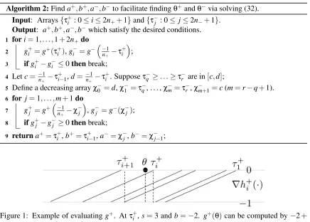
Figure 1: Example of evaluatingg+. Atτ+_i ,s=3 andb=₋2. g+(θ)can be computed by₋2+

3(θ₋τ+_i ). Atτ+_i+1,s=2 andb=₋3.

to the largest possible value such thatθ_∈(τ+_i+1,τ+_i ]and computeg+(θ)byb+s(θ₋τ+_i ). In other words, whenθ>τ+_i , we need to decrementi; and whenθ_≤τ+_i+1 we incrementi. An example is given in Figure 1.

The key operation here is how to update s and b when sliding i. We say iis a head if τ+_i

corresponds to somea+_k (rather thana+_{k −}µ). Otherwise we sayiis a tail. We initialize by setting

i=1,s=1 andb=0. Then the update rule falls in four cases:

• Incrementiandi′=i+1 is a head: update bys′=s+1, andb′=b+s_·1_µ(τ+_i′ −τ+i ). • Incrementiandi′=i+1 is a tail: update bys′=s₋1 andb′=b+s_·1_µ(τ+_i′ −τ+_i ). • Decrementitoi′=i₋1, andiis a head: update bys′=s₋1 andb′=b₋s′_·1_µ(τ+_{i −}τ+_i′). • Decrementitoi′=i₋1, andiis a tail: update bys′=s+1 andb′=b₋s′_·1_µ(τ+_{i −}τ+_i′). Since the query point grows monotonically, the anchor pointionly needs to slide monotonically too. Hence the total computational cost in each stage isO(n+). It is also not hard to see thatican be

initialized toi=2n+, withs=0 andb=−n+. Finally, suppose we store{a+i ,a+i −µ}by an array

Algorithm 3:Computeg+(θ).

Input: A query pointθ.

Output: g+(θ).

1 Initialize:i=1,s=1,b=0. Given{ai}, do this only once at the first call of this function.

Other initializations are also fine, for example,i=2n+, withs=0 andb=−n+.

2 while TRUE do

3 ifτ+_i ≥θthen

4 ifτ+_i+1<θthen returnb+s·1_µ(θ−τ+_i );

5 else

6 b=b+s·1_µ(τ_i++₁−τ+_i ),i=i+1;

7 ifiis a headthens=s+1;elses=s−1;

8 else

9 ifi==1then return0;

10 ifiis a headthens=s−1;elses=s+1;

11 i=i−1,b=b−s·1_µ(τ+_i+1−τ+_i );

4.2 ROCArea_Loss

For theROCArea_{loss, given the optimal ˆβββin (24) one can compute}

∂ ∂wg

⋆

µ(A⊤w) =

1

m

∑

_i,j

ˆ

βi j(xxxj−xxxi) =−

1

m "

∑

i∈P

xxxi

∑

j_∈N

ˆ

βi j !

| {z }

:=γi

−

∑

j_∈N

xxxj

∑

i∈P

ˆ

βi j !

| {z }

:=γj

#

.

If we can efficiently compute allγi andγj, then the gradient can be computed in O(np) time.

Given ˆβi j, a brute-force approach to computeγi andγj takes O(m)time. We exploit the structure

of the problem to reduce this cost to O(nlogn), thus matching the complexity of the separation algorithm in Joachims (2005). Towards this end, we specialize (24) toROCArea_{and write}

g⋆_µ(A⊤w) =max β ββ

1

m

∑

_i,jβi jw ⊤_(xxx

j−xxxi) +

1

m

∑

_i,jβi j− µ

2

∑

_i,jβ 2

i j !

. (33)

Since allβi jare decoupled, their optimal value can be easily found:

ˆ

βi j=median(1,aj−ai,0)

where ai=

1

µm

w⊤xxxi−

1 2

,andaj=

1

µm

w⊤xxxj+

1 2

. (34)

Below we give a high level description of how γi fori∈

P

can be computed; the scheme for

computingγjfor j∈

N

is identical. We omit the details for brevity.

For a giveni, suppose we can divide

N

into three sets

M

_i+,

M

_i, and

M

_i−such that

Algorithm 4:Computeγi,si,tifor alli∈

P

.

Input: Two arrays_{ai:i∈

P

}and

aj: j∈

N

sorted increasingly:ai≤ai+1and

aj≤aj+1.

Output: _{γi,si,ti:i∈

P

}.

1 Initialize:s=t=0,k= j=0 2 foriin 1 ton₊do

3 while j<n₋ ANDaj+1<aido

4 j= j+1;s=s−aj;t=t−a2j

5 whilek<n₋ANDa_k+1≤a_i+1do

6 k=k+1;s=s+ak;t=t+a2_k

7 s_i=s,t_i=t,γ_i= (n₋−1−k)−(k−j)a_i+s

• j_∈

M

_i =_⇒ aj−ai∈[0,1], hence ˆβi j=aj−ai.

• j∈

M

_i− =_⇒ aj−ai<0, hence ˆβi j=0.

Letsi=∑j∈Miaj. Then, clearly

γi=

∑

j∈N

ˆ

βi j=|

M

i+|+

∑

j∈Mi

aj− |

M

i|ai=|

M

i+|+si− |

M

i|ai.

Plugging the optimal ˆβi j into (33) and using (34), we can computeg⋆µ(A⊤w)as

g⋆_µ(A⊤w) =µ

∑

i j

ˆ

βi j(aj−ai)− µ

2

∑

_{i j} ˆ

β2

i j=µ

∑

j∈N

ajγj−

∑

i_∈P

aiγi !

−µ₂

∑

i j

ˆ

β2

i j.

If we defineti:=∑j∈Mia 2

j, then∑i jβˆ2i j can be efficiently computed via

∑

j

ˆ

β2_{i j}=

M

_i++

_∑

j∈Mi

(aj−ai)2=

M

_i++

M

_ia_i2₋2aisi+ti, ∀i∈

P

.

In order to identify the sets

M

_i+,

M

_i,

M

_i−, and computesiandti, we first sort both{ai:i∈

P

}

andaj: j∈

N

. We then walk down the sorted lists to identify for eachithe first and last indices j such that aj−ai ∈[0,1]. This is very similar to the algorithm used to merge two sorted lists,

and takesO(n₋+n+) =O(n)time and space. The rest of the operations for computingγi can be

performed inO(1)time with some straightforward book-keeping. The whole algorithm is presented in Algorithm 4 and its overall complexity is dominated by the complexity of sorting the two lists, which isO(nlogn).

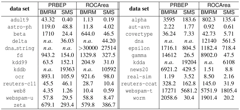
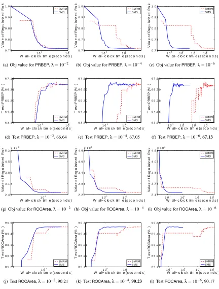
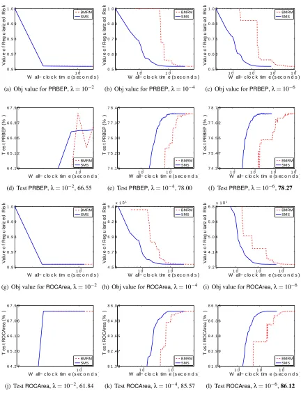
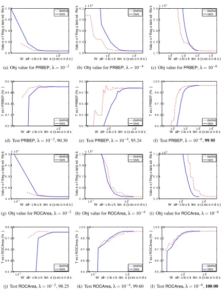
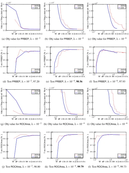
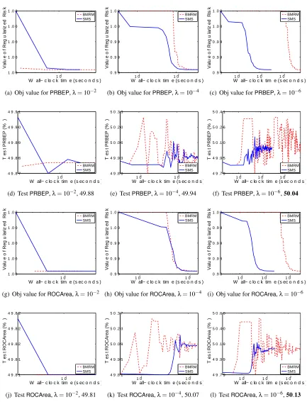
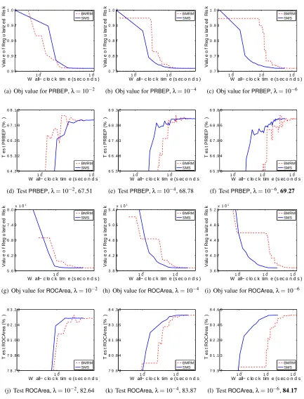
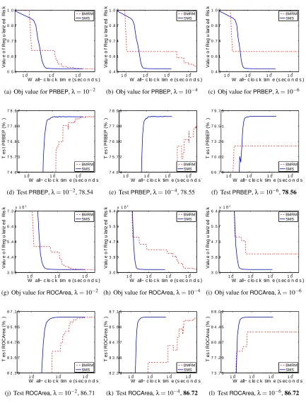
5. Empirical Evaluation

Therefore, what we are specifically interested in is the rate at which the objective function and generalization performance decreases. We will refer to our algorithm as SMS_{, for Smoothing}

for MultivariateScores. As our comparator we use BMRM_{. We downloaded}BMRM _fromhttp:

//users.rsise.anu.edu.au/˜chteo/BMRM.html, and used the default settings in all our experi-ments.

5.1 Data Sets

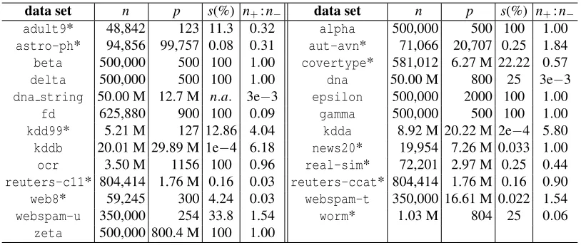
Table 1 summarizes the data sets used in our experiments.adult9,astro-ph,news20,real-sim,

reuters-c11,reuters-ccatare from the same source as in Hsieh et al. (2008). aut-avnis from Andrew McCallum’s home page,6 covertype is from the UCI repository (Frank and Asuncion, 2010), wormis from Franc and Sonnenburg (2008),kdd99is from KDD Cup 1999,7 while web8,

webspam-u, webspam-t,8 as well as the kdda and kddb9 are from the LibSVM binary data col-lection.10 The alpha, beta, delta, dna, epsilon, fd,gamma, ocr, and zeta data sets were all obtained from the Pascal Large Scale Learning Workshop website (Sonnenburg et al., 2008). Since the features ofdnaare suboptimal compared with the string kernels used by Sonnenburg and Franc (2010), we downloaded their original DNA sequence (dna string).11 In particular, we used a weighted degree kernel and two weighted spectrum kernels (one at position 1-59 and one at 62-141, corresponding to the left and right of the splice site respectively), all with degree 8. Following Son-nenburg and Franc (2010), we used the dense explicit feature representations of the kernels, which amounted to 12,670,100 features.

For dna stringand the data sets which were also used by Teo et al. (2010) (indicated by an asterisk in Table 1), we used the training test split provided by them. For the remaining data sets we used 80% of the labeled data for training and the remaining 20% for testing. In all cases, we added a constant feature as a bias.

5.2 Optimization Algorithms

Optimizing the smooth objective functionJµ(w) using the optimization scheme described in

Nes-terov (2005) requires estimating the Lipschitz constant of the gradient of theg⋆_µ(A⊤w). Although it can be automatically tuned by, for example, Beck and Teboulle (2009), extra cost is incurred which slows down the optimization empirically. Therefore, we chose to optimize our smooth ob-jective function using L-BFGS, a widely used quasi-Newton solver (Nocedal and Wright, 1999). We implemented our smoothed loss using PETSc12 and TAO,13 which allow theefficient use of large-scale parallel linear algebra. We used the Limited Memory Variable Metric (lmvm) variant of

6. The data set can be found athttp://www.cs.umass.edu/˜mccallum/data/sraa.tar.gz. 7. The data set can be found athttp://kdd.ics.uci.edu/databases/kddcup99/kddcup99.html.

8.webspam-uis the webspam-unigram andwebspam-tis the webspam-trigram data set. Original data set can be found

athttp://www.cc.gatech.edu/projects/doi/WebbSpamCorpus.html.

9. These data sets were derived from KDD CUP 2010. kddais the first problem algebra 2008 2009 andkddbis the second problem bridge to algebra 2008 2009.

10. The data set can be found athttp://www.csie.ntu.edu.tw/˜cjlin/libsvmtools/datasets/binary.html. 11. The data set can be found athttp://sonnenburgs.de/soeren/projects/coffin/splice_data.tar.xz. 12. The software can be found at http://www.mcs.anl.gov/petsc/petsc-2/index.html. We compiled an

opti-mized version of PETSc (--with-debugging=0) and enabled 64-bit index to run for large data sets such asdnaand

ocr.

data set n p s(%) n+:n− data set n p s(%) n+:n−

adult9* 48,842 123 11.3 0.32 alpha 500,000 500 100 1.00

astro-ph* 94,856 99,757 0.08 0.31 aut-avn* 71,066 20,707 0.25 1.84

beta 500,000 500 100 1.00 covertype* 581,012 6.27 M 22.22 0.57

delta 500,000 500 100 1.00 dna 50.00 M 800 25 3e₋3

dna string 50.00 M 12.7 M n.a. 3e−3 epsilon 500,000 2000 100 1.00

fd 625,880 900 100 0.09 gamma 500,000 500 100 1.00

kdd99* 5.21 M 127 12.86 4.04 kdda 8.92 M 20.22 M 2e−4 5.80

kddb 20.01 M 29.89 M 1e−4 6.18 news20* 19,954 7.26 M 0.033 1.00

ocr 3.50 M 1156 100 0.96 real-sim* 72,201 2.97 M 0.25 0.44

reuters-c11* 804,414 1.76 M 0.16 0.03 reuters-ccat* 804,414 1.76 M 0.16 0.90

web8* 59,245 300 4.24 0.03 webspam-t 350,000 16.61 M 0.022 1.54

webspam-u 350,000 254 33.8 1.54 worm* 1.03 M 804 25 0.06

zeta 500,000 800.4 M 100 1.00

Table 1: Summary of the data sets used in our experiments. nis the total number of examples, p

is the number of features,s is the feature density (% of features that are non-zero), and

n+:n−is the ratio of the number of positive vs negative examples. M denotes a million. A

data set is marked with an asterisk if it is also used by Teo et al. (2010).

L-BFGS which is implemented in TAO. Open-source code, as well as all the scripts used to run our experiments are available for download from Zhang et al. (2012).

5.3 Implementation And Hardware

BothBMRM_andSMS_{are implemented in C++. Sincednaandocrrequire more memory than was}

available on a single machine, we ran bothBMRM_andSMS_{with 16 cores spread across 16 machines}

for these two data sets. Asdna stringemploys a large number of dense features, it would cost a prohibitively large amount of memory. So following Sonnenburg and Franc (2010), we (repeatedly) computed the explicit features whenever it is multiplied with the weight vector www. This entails demanding cost in computation, and therefore we used 32 cores. The other data sets were trained with a single core. All experiments were conducted on theRossmanncomputing cluster at Purdue University,14where each node has two 2.1 GHz 12-core AMD 6172 processors with 48 GB physical memory per node.

5.4 Experimental Setup

We usedλ_∈10−2,10−4,10−6 to test the performance of BMRM_andSMS _{under a reasonably}

wide range ofλ. In line with Chapelle (2007), we observed that solutions with higher accuracy do not improve the generalization performance, and setting ε=0.001 was often sufficient. Accord-ingly, we could setµ=ε/Das suggested by the uniform deviation bound (13). However, this esti-mate is very conservative because in (13) we usedDas an upper bound on the prox-function, while in practice the quality of the approximation depends on the value of the prox-functionaround the optimum. On the other hand, a larger value ofµproffers more strong convexity ingµ, which makes