Maximum Relative Margin and Data-Dependent Regularization
Pannagadatta K. Shivaswamy [email protected]
Tony Jebara [email protected]
Department of Computer Science Columbia University
New York NY 10027 USA
Editor: John Shawe-Taylor
Abstract
Leading classification methods such as support vector machines (SVMs) and their counterparts achieve strong generalization performance by maximizing the margin of separation between data classes. While the maximum margin approach has achieved promising performance, this article identifies its sensitivity to affine transformations of the data and to directions with large data spread. Maximum margin solutions may be misled by the spread of data and preferentially separate classes along large spread directions. This article corrects these weaknesses by measuring margin not in the absolute sense but rather only relative to the spread of data in any projection direction. Maxi-mum relative margin corresponds to a data-dependent regularization on the classification function while maximum absolute margin corresponds to anℓ2norm constraint on the classification func-tion. Interestingly, the proposed improvements only require simple extensions to existing maximum margin formulations and preserve the computational efficiency of SVMs. Through the maximiza-tion of relative margin, surprising performance gains are achieved on real-world problems such as digit, text classification and on several other benchmark data sets. In addition, risk bounds are derived for the new formulation based on Rademacher averages.
Keywords: support vector machines, kernel methods, large margin, Rademacher complexity
1. Introduction
In classification problems, the aim is to learn a classifier that generalizes well on future data from a limited number of training examples. Support vector machines (SVMs) and maximum margin classifiers (Vapnik, 1995; Sch¨olkopf and Smola, 2002; Shawe-Taylor and Cristianini, 2004) have been a particularly successful approach both in theory and in practice. Given a labeled training set, these return a predictor that accurately labels previously unseen test examples. For simple bi-nary classification in Euclidean spaces, this predictor is a function f :Rm→ {±1}estimated from observed training data(xi,yi)ni=1consisting of inputs xi∈Rmand outputs yi∈ {±1}. A linear
func-tion1 f(x):=sign(w⊤x+b)where w∈Rm,b∈Rserves as the decision rule throughout this article. The parameters of the hyperplane(w,b)are estimated by maximizing the margin (e.g., the distance between the hyperplanes defined by w⊤x+b=1 and w⊤x+b=−1) while minimizing a weighted upper bound on the misclassification rate on training data (via so-called slack variables). In practice, the margin is maximized by minimizing 12w⊤w plus an upper bound on the misclassification rate.
1. In this article the dot product w⊤x is used with the understanding that it can be replaced with a generalized inner
While maximum margin classification works well in practice, its solution can easily be perturbed by an (invertible) affine or scaling transformation of the input space. For instance, by transforming all training and testing inputs by an invertible linear transformation, the SVM solution and its re-sulting classification performance can be significantly varied. This is worrisome since an adversary could directly exploit this shortcoming and transform the data to drive performance down; a syn-thetic example showing this effect will be presented in Section 5. Moreover, this phenomenon is not limited to an explicit adversarial setting; it can naturally occur in many real world classification problems, especially in high dimensions. This article will explore such shortcomings in maximum margin solutions (or equivalently, SVMs in the context of this article) which exclusively measure margin by the points near the classification boundary regardless of how spread the remaining data is away from the separating hyperplane. An alternative approach will be followed based on controlling the spread while maximizing the margin. This helps overcome this bias and produces a formulation that is affine invariant. The key is to recover a large margin solution while normalizing the margin by the spread of the data. Thus, margin is measured in a relative sense rather than in the absolute sense. In addition, theoretical results using Rademacher averages support this intuition. The re-sulting classifier will be referred to as the relative margin machine (RMM) and was first introduced by Shivaswamy and Jebara (2009a) with this longer article serving to provide more details, more thorough empirical evaluation and more theoretical support.
Traditionally, controlling spread has been an important theme in classification problems. For in-stance, classical linear discriminant analysis (LDA) (Duda et al., 2000) finds projections of the data so that the inter-class separation is large while within-class scatter is small. However, the spread (or scatter in this context) is estimated by LDA using only simple first and the second order statistics of the data. While this is appropriate if class-conditional densities are Gaussian, second-order statis-tics are inappropriate for many real-world data sets and thus, the classification performance of LDA is typically weaker than that of SVMs. The estimation of spread should not make second-order assumptions about the data and should be tied to the margin criterion (Vapnik, 1995). A similar line of reasoning has been proposed to perform feature selection. Weston et al. (2000) showed that second order tests and filtering methods on features perform poorly compared to wrapper methods on SVMs which more reliably remove features that have low discriminative value. In this prior work, a feature’s contribution to margin is compared to its effect on the radius of the data by com-puting bounding hyper-spheres rather than simple second-order statistics. Unfortunately, there, only axis-aligned feature selection was considered. Similarly, ellipsoidal kernel machines (Shivaswamy and Jebara, 2007) were proposed to normalize data in feature space by estimating bounding hyper-ellipsoids while avoiding second-order assumptions. Similarly, the radius-margin bound has been used as a criterion to tune the hyper-parameters of the SVM (Keerthi, 2002). Another criterion based jointly on ideas from the SVM method as well as Linear Discriminant Analysis has been studied by Zhang et al. (2005). This technique involves first solving the SVM and then solving an LDA problem based on the support vectors that were obtained. While these previous methods showed performance improvements, they relied on multiple-step locally optimal algorithms for interleaving spread information with margin estimation.
is the second order perceptron framework (Cesa-Bianchi et al., 2005) which parallels some of the intuitions underlying the RMM. In an on-line setting, the second order perceptron maintains both a decision rule and a covariance matrix to whiten the data. The mistake bounds it inherits were shown to be better than those of the classical perceptron algorithm. Alternatively, one may consider distributions over classifier solutions which provide a different estimate than the maximum margin setting and have also shown empirical improvements over SVMs (Jaakkola et al., 1999; Herbrich et al., 2001). In recent papers, Dredze et al. (2008) and Crammer et al. (2009a) consider a distribu-tion on the perceptron hyperplane. These distribudistribu-tion assumpdistribu-tions permit update rules that resemble whitening of the data, thus alleviating adversarial affine transformations and producing changes to the basic maximum margin formulation that are similar in spirit to those the RMM provides. In addition, recently, a new batch algorithm called the Gaussian margin machine (GMM) (Crammer et al., 2009b) has been proposed. The GMM maintains a Gaussian distribution over weight vectors for binary classification and seeks the least informative distribution that correctly classifies train-ing data. While the GMM is well motivated from a PAC-Bayesian perspective, the optimization problem itself is expensive involving a log-determinant optimization.
Another alternative route for improving SVM performance includes the use of additional exam-ples. For instance, unlabeled or test examples may be available in semi-supervised or transductive formulations of the SVM (Joachims, 1999; Belkin et al., 2005). Alternatively, additional data that does not belong to any of the classification classes of interest may be available as in the so-called Universum approach (Weston et al., 2006; Sinz et al., 2008). In principle, these methods also change the way margin is measured and the way regularization is applied to the learning problem. While additional data can be helpful in overcoming limitations for many classifiers, this article will be interested in only the simple binary classification setting. The argument is that, without any ad-ditional assumptions beyond the simple classification problem, maximizing margin in the absolute sense may be suboptimal and that maximizing relative margin is a promising alternative.
Further, large margin methods have been successfully applied to a variety of tasks such as pars-ing (Collins and Roark, 2004; Taskar et al., 2004), matrix factorization (Srebro et al., 2005), struc-tured prediction (Tsochantaridis et al., 2005), etc.; in fact, the RMM approach could be readily adapted to such problems. For instance, RMM has been successfully extended to structured predic-tion problems (Shivaswamy and Jebara, 2009b).
The organization of this article is as follows. Motivation from various perspectives are given in Section 2. The relative margin machine formulation is detailed in Section 3 and several variants and implementations are proposed. Generalization bounds for the various function classes are studied in Section 4. Experimental results are provided in Section 5. Finally, conclusions are presented in Section 6. Some proofs and otherwise standard results are provided in the Appendix.
1.1 Notation
Throughout this article, boldface letters indicate vectors/matrices. For two vectors u∈Rm and v∈Rm, u≤v indicates that u
i≤vi for all i from 1 to m. 1, 0 and I denote the vectors of all ones,
2. Motivation
This section provides three different (an intuitive, a probabilistic and an affine transformation based) motivations for maximizing the margin relative to the data spread.
2.1 Intuitive Motivation with a Two Dimensional Example
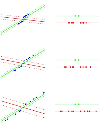
Consider the simple two dimensional data set in Figure 1 where the goal is to separate the two classes of points: triangles and squares. The figure depicts three scaled versions of the two dimensional problem to illustrate potential problems with the large margin solution.
In the topmost plot in the left column of Figure 1, two possible linear decision boundaries separating the classes are shown. The red (or dark shade) solution is the SVM estimate while the green (or light shade) solution is the proposed maximum relative margin alternative. Clearly, the SVM solution achieves the largest margin possible while separating both classes, yet is this necessarily the best solution?
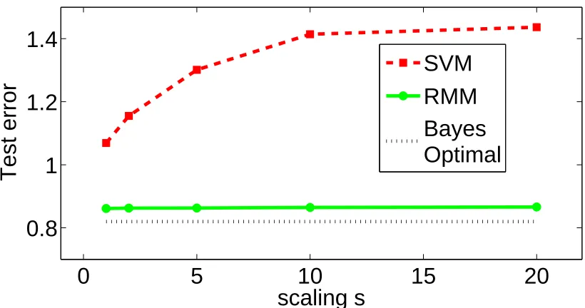
Next, consider the same set of points after a scaling transformation in the second and the third row of Figure 1. Note that all these three problems correspond to the same discrimination problem up to a scaling factor. With progressive scaling, the SVM increasingly deviates from the maximum relative margin solution (green), clearly indicating that the SVM decision boundary is sensitive to affine transformations of the data. Essentially, the SVM produces a family of different solutions as a result of the scaling. This sensitivity to scaling and affine transformations is worrisome. If the SVM solution and its generalization accuracy vary with scaling, an adversary may exploit such scaling to ensure that the SVM performs poorly. Meanwhile, an algorithm producing the maximum relative margin (green) decision boundary could remain resilient to adversarial scaling.
In the previous example, a direction with a small spread in the data produced a good and affine-invariant discriminator which maximized relative margin. Unlike the maximum margin solution, this solution accounts for the spread of the data in various directions. This permits it to recover a solution which has a large margin relative to the spread in that direction. Such a solution would otherwise be overlooked by a maximum margin criterion. A small margin in a correspondingly smaller spread of the data might be better than a large absolute margin with correspondingly larger data spread. This particular weakness in large margin estimation has only received limited attention in previous work.
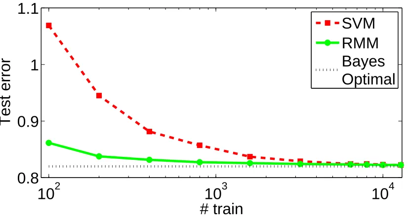
It is helpful to consider the generative model for the above motivating example. Therein, each class was generated from a one dimensional line distribution with the two classes on two parallel lines. In this case, the maximum relative margin (green) decision boundary should obtain zero test error even if it is estimated from a finite number of examples. However, for finite training data, the SVM solution will make errors and will do so increasingly as the data is scaled further. While it is possible to anticipate these problems and choose kernels or nonlinear mappings to correct for them in advance, this is not necessarily practical. The right mapping or kernel is never provided in advance in realistic settings. Instead, one has to estimate kernels and nonlinear mappings, a difficult endeavor which can often exacerbate the learning problem. Similarly, simple data preprocessing (affine whitening to make the data set zero-mean and unit-covariance or scaling to place the data into a zero-one box) can also fail, possibly because of estimation problems in recovering the correct transformation (this will be shown in real-world experiments).
balanced with the goal of simultaneously minimizing the spread of the projected data, for instance, by bounding the spread |w⊤x+b|. This will allow the linear classifier to recover large margin solutions not in the absolute sense but rather relative to the spread of the data in that projection direction.
In the case of a kernel such as the RBF kernel, the points are first mapped to a space so that all the input examples are unit vectors (i.e., hφ(x),φ(x)i=1). Note that the intuitive motivation proposed here still applies in such cases. No matter how they are mapped initially, a large margin solution still projects these points to the real line where the margin of separation is maximized. However, the spread of the projection can still vary significantly among the different projection directions. Given the above motivation, it is important to achieve a large margin relative to the spread of the projections even in such situations. Furthermore, experiments will support this intuition with dramatic improvements on many real problems and with a variety of kernels (including radial basis function and polynomial kernels).
2.2 Probabilistic Motivation
In this subsection, an informal motivation is provided to illustrate why maximizing relative margin may be helpful. Suppose(xi,yi)ni=1are drawn independently and identically (iid) from a distribution
D
. A classifier w∈Rmis sought which will produce low error on future unseen examples according to the decision rule ˆy=sign(w⊤x). An alternative criterion is that the classifier should produce a large value ofηaccording to the following expression:Pr
(x,y)∼D h
yw⊤x≥0 i
≥η,
where w∈Rm is the classifier. One way to ensure the above constraint is by requiring that the following inequality hold:
ED[yw⊤x]≥
r η
1−η q
VD[yw⊤x]. (1)
A proof of the above claim for a general distribution can be found in Shivaswamy et al. (2006). In fact, Gaussian margin machines (Crammer et al., 2009b) start with a similar motivation but assume a Gaussian distribution on the classifier.
According to (1), achieving a low probability of error requires the projections to have a large mean and a small variance. The mean and variance for the true distribution
D
may be unavailable, however, the empirical counterparts of these quantities are available and known to be concentrated. The above inequality is used as a loose motivation. Instead of precisely finding low variance and high mean projections, this paper implements this intuition by trading off between large margin and small projections of the data while correctly classifying most of the examples with a hinge loss.2.3 Motivation From an Affine Invariance Perspective
ratio of the margin to the radius of the data (Vapnik, 1995). Similarly, Rademacher generalization bounds (Shawe-Taylor and Cristianini, 2004) also consider the ratio of the trace of the kernel matrix to the margin. Here the radius of the data refers to an R such that||x|| ≤R for all x drawn from a distribution.
Instead of learning a classification rule, the optimization problem considered in this section will recover an affine transformation which achieves a large margin from a fixed decision rule while also achieving small radius. Assume the classification hyperplane is given a priori via the decision boundary w⊤0x+b0=0 with the two supporting margin hyperplanes w⊤0x+b0=±ρ. Here, w0∈Rm can be an arbitrary unit vector and b0 is an arbitrary scalar. Consider the problem of mapping all the training points (by an affine transformation x→Ax+b,A∈Rm×m,b∈Rm) so that the mapped
points (i.e., Axi+b) satisfy the classification constraints w⊤0x+b0=±ρwhile producing small radius, √R. The choice of w0 and b0 is arbitrary since the affine transformation can completely compensate for it. For brevity, denote by ˜A= [A b]and ˜x= [x⊤1]⊤. With this notation, the affine transformation learning problem is formalized by the following optimization:
min ˜
A,R,ρ −ρ+ER (2)
yi(w⊤0A˜x˜ i+b0)≥ρ, ∀1≤i≤n
1 2(A˜x˜ i)
⊤(A˜x˜ i)≤R ∀1≤i≤n.
The parameter E trades off between the radius of the affine transformed data and the margin2that will be obtained. The following Lemma shows that this affine transformation learning problem is basically equivalent to learning a large margin solution with a small spread.
Lemma 1 The solution ˜A∗to (2) is a rank one matrix.
Proof Consider the Lagrangian of the above problem with Lagrange multipliersα,λ,≥0:
L
(A˜,ρ,R,α,λ) =−ρ+ER−n
∑
i=1
αi(yi(w⊤0A˜x˜ i+b0)−ρ)
+
n
∑
i=1
λi(
1 2(A˜x˜ i)
⊤(A˜x˜ i)−R).
Differentiating the above Lagrangian with respect to A gives the following expression:
∂
L
(A˜,ρ,R,α,λ)∂A˜ =−
n
∑
i=1
αiyiw0˜x⊤i +A˜ n
∑
i=1
λi˜xi˜x⊤i . (3)
From (3), at optimum,
˜ A∗
n
∑
i=1
λi˜xi˜x⊤i =− n
∑
i=1
αiyiw0˜x⊤i .
It is therefore clear that ˜A∗ can always be chosen to have rank one since the right hand side of the expression is just an outer product of two vectors.
Lemma 1 gives further intuition on why one should limit the spread of the recovered classifier. Learning a transformation matrix ˜A so as to maximize the margin while minimizing the radius given an a priori hyperplane(w0,b0)is no different from learning a classification hyperplane(w,b)with a large margin as well as a small spread. This is because the rank of the affine transformation ˜A∗ is one; thus, ˜A∗merely maps all the points ˜xionto a line achieving a certain marginρbut also
lim-iting the output or spread. This means that finding an affine transformation which achieves a large margin and small radius is equivalent to finding a w and b with a large margin and with projections constrained to remain close to the origin. Thus, the affine transformation learning problem comple-ments the intuitive argucomple-ments in Section 2.1 and also suggests that the learning algorithm should bound the spread of the data.
3. From Absolute Margin to Relative Margin
This section will provide an upgrade path from the maximum margin classifier (or SVM) to a max-imum relative margin formulation. Given independent identically distributed examples(xi,yi)ni=1 where xi∈Rmand yi∈ {±1}are drawn from Pr(x,y), the support vector machine primal
formula-tion is as follows:
min
w,b,ξ 1 2kwk
2+C
∑
ni=1
ξi (4)
s.t. yi(w⊤xi+b)≥1−ξi, ξi≥0 ∀1≤i≤n.
The above is an easily solvable quadratic program (QP) and maximizes the margin by minimizing
kwk2. Since real data is seldom separable, slack variables (ξi) are used to relax the hard
classifi-cation constraints. Thus, the above formulation maximizes the margin while minimizing an upper bound on the number of classification errors. The trade-off between the two quantities is controlled by the parameter C. Equivalently, the following dual of the formulation (4) can be solved:
max
α n
∑
i=1
αi−
1 2
n
∑
i=1
n
∑
j=1
αiαjyiyjx⊤i xj (5)
s.t.
n
∑
i=1
αiyi=0
0≤αi≤C ∀1≤i≤n.
Lemma 2 The formulation in (5) is invariant to a rotation of the inputs.
Proof Replace each xi with Axiwhere A is a rotation matrix such that A∈Rm×mand A⊤A=I. It
is clear that the dual remains the same.
However, the dual is not the same if A is more general than a rotation matrix, for instance, if it is an arbitrary affine transformation.
The above classification framework can also handle non-linear classification readily by making use of Mercer kernels. A kernel function k :Rm×Rm→Rreplaces the dot products x⊤
i xj in (5).
The kernel function k is such that k(xi,xj) =
φ
(xi),φ(xj)
non-linear solution in the input space. In the rest of this article, K∈Rn×ndenotes the Gram matrix whose individual entries are given by Ki j=k(xi,xj). When applying Lemma 2 on a kernel defined
feature space, the affine transformation is onφ(xi)and not on xi.
3.1 The Whitened SVM
One way of limiting sensitivity to affine transformations while recovering a large margin solution is to whiten the data with the covariance matrix prior to estimating the SVM solution. This may also reduce the bias towards regions of large data spread as discussed in Section 2. Denote by
Σ= 1 n
n
∑
i=1 xix⊤i −
1 n2 n
∑
i=1 xi n∑
j=1x⊤j, and µ=1 n
n
∑
i=1 xi,
the sample covariance and sample mean, respectively. Now, consider the following formulation calledΣ-SVM:
min
w,b,ξ 1−D
2 kwk 2+D
2kΣ
1
2wk2+C
n
∑
i=1
ξi (6)
s.t. yi(w⊤(xi−µ) +b)≥1−ξi,ξi≥0 ∀1≤i≤n
where 0≤D≤1 is an additional parameter that trades off between the two regularization terms. When D=0, (6) gives back the usual SVM primal (although on translated data). The dual of (6) can be shown to be:
max
α n
∑
i=1
αi−
1 2
n
∑
i=1
αiyi(xi−µ)⊤((1−D)I+DΣ)−1 n
∑
j=1
αjyj(xj−µ) (7)
s.t.
n
∑
i=1
αiyi=0
0≤αi≤C ∀1≤i≤n.
It is easy to see that the above formulation (7) is translation invariant and tends to an affine invariant solution when D tends to one. However, there are some problems with this formulation. First, the whitening process only considers second order statistics of the input data which may be inappro-priate for non-Gaussian data sets. Furthermore, there are computational difficulties associated with whitening. Consider the following term:
(xi−µ)⊤((1−D)I+DΣ)−1(xj−µ).
When 0<D<1, it can be shown, by using the Woodbury matrix inversion formula, that the above term can be kernelized as
ˆk(xi,xj) =
1
1−D k(xi,xj)− K⊤i 1
n −
K⊤j1
n +
1⊤K1 n2
!
−1 1 −D
Ki−
K1 n ⊤ I n− 11⊤ n2
1−D
D I+K
I n− 11⊤ n2 −1 Kj−
K1 n
where Kiis the ithcolumn of K. This implies that theΣ-SVM can be solved merely by solving (5)
after replacing the kernel with ˆk(xi,xj)as defined above. Note that the above formula involves a
matrix inversion of size n, making the kernel computation alone
O
(n3). Even performing whitening as a preprocessing step in the feature space would involve this matrix inversion which is often computationally prohibitive.3.2 Relative Margin Machines
While the above Σ-SVM does address some of the issues of data spread, it made second order assumptions to recoverΣand involved a cumbersome matrix inversion. A more direct and efficient approach to control the spread is possible and will be proposed next.
The SVM will be modified such that the projections on the training examples remain bounded. A parameter will also be introduced that helps trade off between large margin and small spread of the projection of the data. This formulation will initially be solved by a quadratically constrained quadratic program (QCQP) in this section. The dual of this formulation will also be of interest and yield further geometric intuitions.
Consider the following formulation called the relative margin machine (RMM):
min
w,b
1 2kwk
2+C
∑
ni=1
ξi (8)
s.t. yi(w⊤xi+b)≥1−ξi, ξi≥0 ∀1≤i≤n
1 2(w
⊤x
i+b)2≤
B2
2 ∀1≤i≤n.
This formulation is similar to the SVM primal (4) except for the additional constraints12(w⊤xi+
b)2≤B2
2. The formulation has one extra parameter B in addition to the SVM parameter C. When B is large enough, the above QCQP gives the same solution as the SVM. Also note that only settings of B>1 are meaningful since a value of B less than one would prevent any training examples from clearing the margin, that is, none of the examples could satisfy yi(w⊤xi+b)≥1 otherwise. Let wC
and bCbe the solutions obtained by solving the SVM (4) for a particular value of C. It is clear, then,
that B>maxi|wC⊤xi+bC|, makes the constraint on the second line in the formulation (8) inactive
for each i and the solution obtained is the same as the SVM estimate. This gives an upper threshold for the parameter B so that the RMM solution is not trivially identical to the SVM solution.
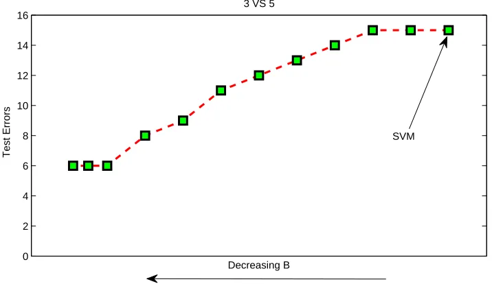
As B is decreased, the RMM solution increasingly differs from the SVM solution. Specifically, with a smaller B, the RMM still finds a large margin solution but with a smaller projection of the training examples. By trying different B values (within the aforementioned thresholds), different large relative margin solutions are explored. It is helpful to next consider the dual of the RMM problem.
The Lagrangian of (8) is given by:
L
(w,b,α,λ,β) =1 2kwk2+C
∑
ni=1
ξi− n
∑
i=1
αi
yi(w⊤xi+b)−1+ξi
−
n
∑
i=1
βiξi
+
n
∑
i=1
λi
1 2(w
⊤x
i+b)2−
1 2B
2
where α,β,λ≥0 are the Lagrange multipliers corresponding to the constraints. Differentiating with respect to the primal variables and equating to zero produces:
(I+
n
∑
i=1
λixix⊤i )w+b n
∑
i=1
λixi= n
∑
i=1
αiyixi,
1 λ⊤1(
n
∑
i=1
αiyi− n
∑
i=1
λiw⊤xi) =b,
αi+βi=C ∀1≤i≤n.
Denoting by
Σλ=
n
∑
i=1
λixix⊤i −
1 λ⊤1
n
∑
i=1
λixi n
∑
j=1
λjx⊤j, and µλ=
1 λ⊤1
n
∑
i=1
λixi,
the dual of (8) can be shown to be:
max
α,λ n
∑
i=1
αi−
1 2
n
∑
i=1
αiyi(xi−µλ)⊤(I+Σλ)−1 n
∑
j=1
αjyj(xj−µλ) +
1 2B
2
∑
ni=1
λi (9)
s.t. 0≤αi≤C λi≥0 ∀1≤i≤n.
Moreover, the optimal w can be shown to be:
w= (I+Σλ)−1 n
∑
i=1
αiyi(xi−µλ).
Note that the above formulation is translation invariant since µλ is subtracted from each xi. Σλ
corresponds to a shape matrix (which is potentially low rank) determined by xi’s that have non-zero
λi. From the Karush-Kuhn-Tucker (KKT) conditions of (8) it is clear thatλi(12(w⊤xi+b)2−B
2
2) = 0. Consequently λi >0 implies (12(w⊤xi+b)2−B
2
2) =0. Notice the similarity in the two dual formulations in (7) and (9); both formulations look similar except for the choice ofµandΣwhich transform the inputs. The RMM in (9) whitens data with the matrix(I+Σλ)while simultaneously solving an SVM-like classification problem. While this is similar in spirit to theΣ-SVM, the matrix
(I+Σλ)is being estimated directly to optimize the margin with a small data spread. TheΣ-SVM
only whitens data as a preprocessing independently of the margin and the labels. TheΣ-SVM is equivalent to the RMM only in the rare situation when allλi=t for some t which makes theµλand
Σλin the RMM andΣ-SVM identical up to a scaling factor.
In practice, the above formulation will not be solved since it is computationally impractical. Solving (9) requires semi-definite programming (SDP) which prevents the method from scaling beyond a few hundred data points. Instead, an equivalent optimization will be used which gives the same solution but only requires quadratic programming. This is achieved by simply replacing the constraint 12(w⊤xi+b)2≤21B2with the two equivalent linear constraints: (w⊤xi+b)≤B and −(w⊤xi+b)≤B. With these linear constraints replacing the quadratic constraint, the problem is
3.3 Fast Implementation
Once the quadratic constraints have been replaced with linear constraints, the RMM is merely a quadratic program which admits many fast implementation schemes. It is now possible to adapt previous fast SVM algorithms in the literature to the RMM. In this section, the SVMlight(Joachims, 1998) approach will be adapted to the following RMM optimization problem
min
w,b
1 2kwk
2+C
∑
ni=1
ξi (10)
s.t. yi(w⊤xi+b)≥1−ξi, ξi≥0 ∀1≤i≤n
w⊤xi+b≤B ∀1≤i≤n
−w⊤xi−b≤B ∀1≤i≤n.
The dual of (10) can be shown to be the following:
max
α,λ,λ∗ −
1
2(α•y−λ+λ
∗)⊤K(α•y−λ+λ∗) +α⊤1−Bλ⊤1−Bλ∗⊤1 (11)
s.t.α⊤y−λ⊤1+λ∗⊤1=0 0≤α≤C1
λ,λ∗≥0,
where the operator•denotes the element-wise product of two vectors.
The QP in (11) is solved in an iterative way. In each step, only a subset of the dual variables are optimized. For instance, in a particular iteration, take q, r and s ( ˜q, ˜r and ˜s) to be indices of the free (fixed) variables inα,λandλ∗ respectively (ensuring that q∪q˜={1,2, . . .n}and q∩q˜= /0and proceeding similarly for the other two indices). The optimization over the free variables in that step can then be expressed as:
max
αq,λr,λ∗
s
−12
αq•yq
λr
λ∗s
⊤
Kqq −Kqr Kqs −Krq Krr −Krs
Ksq −Ksr Kss
αq•yq
λr
λ∗s
(12)
−12
αq•yq
λr
λ∗s
⊤
Kq ˜q −Kq˜r Kq ˜s −Kr ˜q Kr ˜r −Kr ˜s
Ks ˜q −Ks˜r Ks ˜s
αq˜•yq˜ λ˜r λ∗s˜
+α⊤q1−Bλ⊤r1−Bλ∗⊤s 1
s.t.α⊤qyq−λr⊤1+λ∗⊤s 1=−α⊤q˜yq˜+λ⊤˜r1−λ∗⊤s˜ 1, 0≤αq≤C1,
λr,λ∗s≥0.
the current solution (b is determined by the KKT conditions just as with SVMs), then:
∀i s.t. 0<αi<C : b−ε≤yi−( n
∑
j=1
(αjyj−λj+λ∗j)k(xi,xj))≤b+ε
∀i s.t.αi=0 : yi(
n
∑
j=1
(αjyj−λj+λ∗j)k(xi,xj) +b)≥1−ε
∀i s.t.αi=C : yi(
n
∑
j=1
(αjyj−λj+λ∗j)k(xi,xj) +b)≤1+ε
∀i s.t.λi>0 : B−ε≤(
n
∑
j=1
(αjyj−λj+λ∗j)k(xi,xj) +b)≤B+ε
∀i s.t.λi=0 : (
n
∑
j=1
(αjyj−λj+λ∗j)k(xi,xj) +b)≤B−ε
∀i s.t.λ∗i >0 : B−ε≤ −(
n
∑
j=1
(αjyj−λj+λ∗j)k(xi,xj) +b)≤B+ε
∀i s.t.λ∗i =0 : −(
n
∑
j=1
(αjyj−λj+λ∗j)k(xi,xj) +b)≤B−ε.
In each step of the algorithm, a small sub-problem of the structure of (12) is solved. To select the free variables, these conditions are checked to find the worst violating variables both from the top of the violation list and from the bottom. The selected variables are optimized by solving (12) while keeping the other variables fixed. Since only a small QP is solved in each step, the cubic time scaling behavior is circumvented for improved efficiency. A few other book-keeping tricks have also been adapted from SVMlight to yield other minor improvements.
Denote by p the number of elements chosen in each step of the optimization (i.e., p=|q|+
|r|+|s|). The QP in each step takes
O
(p3)and updating the prediction values to compute the KKT violations takesO
(nq)time. Sorting the output values to choose the most violated constraints takesO
(n log(n))time. Thus, the total time taken in each iteration of the algorithm isO
(p3+n log(n) + nq). Empirical running times are provided in Section 5 for a digit classification problem.Many other fast SVM solvers could also be adapted to the RMM. Recent advances such as the cutting plane SVM algorithm (Joachims, 2006), Pegasos (Shalev-Shwartz et al., 2007) and so forth are also applicable and are deferred for future work.
3.4 Variants of the RMM
min
w,b,ξ,t≥1 1 2kwk
2+C
∑
ni=1
ξi+Dt (13)
s.t. yi(w⊤xi+b)≥1−ξi, ξi≥0 ∀1≤i≤n,
+ (w⊤xi+b)≤t ∀1≤i≤n, −(w⊤xi+b)≤t ∀1≤i≤n.
Note that (13) has a parameter D instead of the parameter B in (10). The two optimization problems are equivalent in the sense that for every value of B in (10), it is possible to have a corre-sponding D such that both optimization problems give the same solution.
Further, in some situations, a hard constraint bounding the outputs as in (13) can be detrimental due to outliers. Thus, it might be required to have a relaxation on the bounding constraints as well. This motivates the following relaxed version of (13):
min
w,b,ξ,t≥1 1 2kwk
2+C
∑
ni=1
ξi+D(t+
ν
n
n
∑
i=1
(τi+τ∗i)) (14)
s.t. yi(w⊤xi+b)≥1−ξi, ξi≥0 ∀1≤i≤n,
+ (w⊤xi+b)≤t+τi ∀1≤i≤n, −(w⊤xi+b)≤t+τ∗i ∀1≤i≤n.
In the above formulation,νcontrols the fraction of outliers. It is not hard to derive the dual of the above to express it in kernelized form.
4. Risk Bounds
This section provides generalization guarantees for the classifiers of interest (the SVM, Σ-SVM and RMM) which all produce decision3boundaries of the form w⊤x=0 from a limited number of examples. In the SVM, the decision boundary is found by minimizing a combination of w⊤w and an upper bound on the number of errors. This minimization is equivalent to choosing a function g(x) =w⊤x from a set of linear functions with boundedℓ2norm. Therefore, with a suitable choice of E, the SVM solution chooses the function g(·)from the set{x→w⊤x|12w⊤w≤E}.
By measuring the complexity of the function class being explored, it is possible to derive gen-eralization guarantees and risk bounds. A natural measure of how complex a function class is the Rademacher complexity which has been fruitful in the derivation of generalization bounds. For SVMs, such results can be found in Shawe-Taylor and Cristianini (2004). This section continues in the same spirit and defines the function classes and their corresponding Rademacher complexi-ties for slightly modified versions of the RMM as well as theΣ-SVM. Furthermore, these will be used to provide generalization guarantees for both classifiers. The style and content of this section closely follows that of Shawe-Taylor and Cristianini (2004).
The function classes for the RMM andΣ-SVM will depend on the data. Thus, these both entail so-called data-dependent regularization which is not quite as straightforward as the function classes explored by SVMs. In particular, the data involved in defining data-dependent function classes will
be treated differently and referred to as landmarks to distinguish them from the training data. Land-mark data is used to define the function class while training data is used to select a specific function from the class. This distinction is important for the following theoretical derivations. However, in practical implementations, both theΣ-SVM and the RMM may use the training data to both define the function class and to choose the best function within it. Thus, the distinction between landmark data and training data is merely a formality for deriving generalization bounds which require inde-pendent sets of examples for both stages. Ultimately, however, it will be possible to still provide generalization guarantees that are independent of the particular landmark examples. Details of this argument are provided in Section 4.6. For this section, however, it is assumed that, in parallel with the training data, a separate data set of landmarks is provided to define the function class for the RMM and theΣ-SVM.
4.1 Function Class Definitions
Consider the training data set(xi,yi)ni=1with xi∈Rmand yi∈ {±1}which are drawn independently
and identically distributed (iid) from an unknown underlying distribution P[(x,y)]denoted as
D
. The features of the training examples above are denoted by the set S={x1, . . . ,xn}.Given a choice of the parameter E in the SVM (where E plays the role of the regularization parameter), the set of linear functions the SVM considers is:
Definition 3
F
E :={x→w⊤x|12w⊤w≤E}.The RMM maximizes the margin while also limiting the spread of projections on the training data. It effectively considers the following function class:
Definition 4
H
SE,D:={x→w⊤x|
¯
D
2w⊤w+
D
2(w⊤xi)
2≤E∀1≤i≤n}.
Above, take ¯D :=1−D and 0<D<1 trades off between large margin and small spread on the projections.4Since the above function class depends on the training examples, standard Rademacher analysis, which is straightforward for the SVM, is no longer applicable. Instead, define another function class for the RMM using a distinct set of landmark examples.
A set V={v1, . . . ,vnv} drawn iid from the same distribution P[x], denoted as
D
x, is used asthe landmark examples. With these landmark examples, the modified RMM function class can be written as:
Definition 5
H
VE,D:={x→w⊤x|
¯
D
2w⊤w+
D
2(w⊤vi)2≤E∀1≤i≤nv}.
Finally, function classes that are relevant for theΣ-SVM are considered. These limit the average projection rather than the maximum projection. The data-dependent function class is defined as below:
Definition 6
G
SE,D:={x→w⊤x|
¯
D
2w⊤w+
D
2n∑
n
i=1(w⊤xi)2≤E}.
A different landmark set U={u1, . . . ,un}, again drawn iid from
D
x, is used in defining thecorresponding landmark function class:
Definition 7
G
UB,D:={x→w⊤x|
¯
D
2w⊤w+
D
2n∑
n
i=1(w⊤ui)2≤B}.
Note that the parameter E is fixed in
H
VE,Dbut nv may be different from n. In the case of
G
BU,D,the number of landmarks is the same(n)as the number of training examples but the parameter B is used instead of E. These distinctions are intentional and will be clarified in subsequent sections.
4.2 Rademacher Complexity
In this section the Rademacher complexity of the aforementioned function classes are quantified by bounding the empirical Rademacher complexity. Rademacher complexity measures the richness of a class of real-valued functions with respect to a probability distribution (Bartlett and Mendelson, 2002; Shawe-Taylor and Cristianini, 2004; Bousquet et al., 2004).
Definition 8 For a sample S={x1,x2, . . . ,xn}generated by a distribution on x and a real-valued
function class
F
with domain x, the empirical Rademacher complexity5ofF
isˆ
R(
F
):=Eσ" sup
f∈F 2 n n
∑
i=1σif(xi)
#
where σ={σ1, . . .σn} are independent random variables that take values +1 or −1 with equal
probability. Moreover, the Rademacher complexity of
F
is: R(F
):=ESˆ R(
F
).
A stepping stone for quantifying the true Rademacher complexity is obtained by considering its empirical counterpart.
4.3 Empirical Rademacher Complexity
In this subsection, upper bounds on the empirical Rademacher complexities are derived for the previously defined function classes. These bounds provide insights on the regularization properties of the function classes for the sample S={x1,x2, . . .xn}.
Theorem 9 ˆR(
F
E)≤T0:= 2√ 2E
n
p
tr(K),where tr(K) is the trace of the Gram matrix of the ele-ments in S.
Proof
ˆ
R(
F
E) =Eσ" sup
f∈FE
2 n n
∑
i=1σif(xi)
# =2 nEσ
" max ||w||≤√2E
w⊤ n
∑
i=1σixi
# ≤2 √ 2E
n Eσ
" n
∑
i=1σixi
# =2 √ 2E
n Eσ
n
∑
i=1
σix⊤i n
∑
j=1
σjxj
!12
≤2 √
2E
n Eσ
"
n
∑
i,j=1
σiσjx⊤i xj
#!12
= 2
√
2E n
p tr(K).
The proof uses Jensen’s inequality on the function√·and the fact thatσiandσj are random
vari-ables taking values+1 or −1 with equal probability. Thus, when i6= j, Eσ[σiσjx⊤i xi] =0 and,
otherwise, Eσ[σiσix⊤i xi] =Eσ[x⊤i xi] =x⊤i xi. The result follows from the linearity of the
expecta-tion operator.
Roughly speaking, by keeping E small, the classifier’s ability to fit arbitrary labels is reduced. This is one way to motivate a maximum margin strategy. Note thatptr(K)is a coarse measure of the spread of the data. However, most SVM formulations do not directly optimize this term. This motivates to next consider two new function classes.
Theorem 10 ˆR(
H
VE,D)≤T2(V,S), where for any training set
B
and landmark6setA
, T2(A
,B):=minλ≥0 |B1|∑x∈Bx⊤ DI¯ ∑u∈Aλu+D∑u∈Aλuuu⊤
−1
x+2E|B|∑u∈Aλu.
Proof Start with the definition of the empirical Rademacher complexity:
ˆ
R(
H
EV,D) =Eσ"
sup
w:12(Dw¯ ⊤w+D(w⊤vi)2)≤E
2 n n
∑
i=1σi(w⊤xi)
# .
Consider the supremum inside the expectation. Depending on the sign of the term inside | · |, the above corresponds to either a maximization or a minimization. Without loss of generality, consider the case of maximization. When a minimization is involved, the value of the objective still remains the same. The supremum is recovered by solving the following optimization problem:
max
w w
⊤
∑
ni=1
σixi s.t.
1 2(Dw¯
⊤w+D(w⊤v
i)2)≤E ∀1≤i≤nv. (15)
Using Lagrange multipliersλ1≥0, . . .λnv≥0, the Lagrangian of (15) is:
L
(w,λ) =−w⊤∑n
i=1σixi+
∑nv
i=1λi 12 Dw¯ ⊤w+D(w⊤vi)2
−E.Differentiating this with respect to the primal variable w and equating it to zero gives: w=Σ−1
λ,D∑ n
i=1σixi, whereΣλ,D:=D¯∑ni=v1λiI+D∑ni=v1λiviv⊤i .
Substitut-ing this w in
L
(w,λ)gives the dual of (15):min
λ≥0 1 2
n
∑
i=1
σix⊤i Σ−λ,1D n
∑
j=1
σjxj+E nv
∑
i=1
λi.
This permits the following upper bound on the empirical Rademacher complexity since the primal and the dual objectives are equal at the optimum:
ˆ
R(
H
EV,D) =2 nEσ
" min
λ≥0 1 2
n
∑
i=1
σix⊤i Σ−λ,1D n
∑
j=1
σjxj+E nv
∑
i=1 λi # ≤minλ≥0 2 nEσ
" 1 2 n
∑
i=1σix⊤i Σ−λ,1D n
∑
j=1
σjxj+E nv
∑
i=1 λi # ≤minλ≥0 1 n
n
∑
i=1 x⊤i Σ−1
λ,Dxi+
2 nE
nv
∑
i=1
λi=T2(V,S).
On line one, the expectation is over the minimizers overλ; this is less than first taking the expecta-tion and then minimizing overλin line two. Then, simply recycle the arguments used in Theorem 9 to handle the expectation overσ.
6. T2(A,B)has been defined on generic sets. When an already defined set, such as V (with a known number nvof
Theorem 11 ˆR(
G
UB,D)≤T1(U,S), where for any training set
B
and landmark setA
, T1(A
,B):=2√2B |B|
∑x∈Bx⊤
¯
DI+|AD|∑u∈Auu⊤ −1
x 12
.
Proof The proof is similar to the one for Theorem 10.
Thus, the empirical Rademacher complexities of the function classes of interest are bounded using the functions T0, T1(U,S)and T2(V,S). For both
F
E andG
EU,D, the empirical Rademachercomplexity is bounded by a closed-form expression. For
H
VE,D, optimizing over the Lagrange
multi-pliers (i.e., theλ’s) can further reduce the upper bound on empirical Rademacher complexity. This can yield advantages over both
F
E andG
EU,Din many situations and the overall shape ofΣλ,Dplaysa key role in determining the overall bound; this will be discussed in Section 4.7. Note that the upper bound T2(V,S)is not a closed-form expression in general but can be evaluated in polynomial time using semi-definite programming by invoking Schur’s complement lemma as shown by Boyd and Vandenberghe (2003).
4.4 From Empirical to True Rademacher Complexity
By definition 8, the empirical Rademacher complexity of a function class is dependent on the data sample, S. In many cases, it is not possible to give exact expressions for the Rademacher com-plexity since the underlying distribution over the data is unknown. However, it is possible to give probabilistic upper bounds on the Rademacher complexity. Since the Rademacher complexity is the expectation of its empirical estimate over the data, by a straightforward application of McDiarmid’s inequality (Appendix A), it is possible to show the following:
Lemma 12 Fixδ∈(0,1). With probability at least 1−δover draws of the samples S the following holds for any function class
F
:R(
F
)≤Rˆ(F
) +2 rln(2/δ)
2n (16)
and,
ˆ
R(
F
)≤R(F
) +2 rln(2/δ)
2n . (17)
At this point, the motivation for introducing the landmark sets U and V becomes clear. The in-equalities (16) and (17) do not hold when the function class
F
is dependent on the set S. Specifically, using the sample S instead of the landmarks breaks the required iid assumptions in the derivation of (16) and (17). Thus neither Lemma 12, nor any of the results in Section 4.5 are sound for the function classesG
SB,Dand
H
ES,D.4.5 Generalization Bounds
Theorem 13 Let
F
be a class of functions mapping Z to[0,1]; let{z1, . . . ,zn}be drawn from thedomain Z independently and identically distributed (iid) according to a probability distribution
D
. Then, for any fixedδ∈(0,1), the following bound holds for any f ∈F
with probability at least 1−δover random draws of a set of examples of size n:ED[f(z)]≤Eˆ[f(z)] +Rˆ(
F
) +3 rln(2/δ)
2n . (18)
Similarly, under the same conditions as above, with probability at least 1−δ,
ˆ
E[f(z)]≤ED[f(z)] +Rˆ(
F
) +3 rln(2/δ)
2n . (19)
Inequality (18) can be found in Shawe-Taylor and Cristianini (2004) and inequality (19) is obtained by a simple modification of the proof in Shawe-Taylor and Cristianini (2004). The following theo-rem, found in Shawe-Taylor and Cristianini (2004), gives a probabilistic upper bound on the future error rate based on the empirical error and the function class complexity.
Theorem 14 Fixγ>0. Let
F
be the class of functions fromRm× {±1} →Rgiven by f(x,y) =−yg(x). Let {(x1,y1), . . . ,(xn,yn)} be drawn iid from a probability distribution
D
. Then, withprobability at least 1−δover the samples of size n, the following bound holds:
Pr
D[y6=sign(g(x))]≤ 1 nγ
n
∑
i=1
ξi+
2
γRˆ(
F
) +3r
ln(2/δ)
2n , (20)
whereξi=max(0,1−yig(xi))are the so-called slack variables.
The upper bounds that were derived in Section 4.2, namely: T0, T1(U,S)and T2(V,S)can now be inserted into (20) to give generalization bounds for each class of interest. However, a caveat remains since a separate set of landmark data was necessary to provide such generalization bounds. The next section provides steps to eliminate the landmark data set from the bound.
4.6 Stating Bounds Independently of Landmarks
Note that the original function classes were defined using landmark examples. However, it is pos-sible to eliminate these and state the generalization bounds independent of the landmark examples on function classes defined on the training data. Landmarks are eliminated from the generalization bounds in two steps. First, the empirical Rademacher complexities are shown to be concentrated and, second, the function classes defined using landmarks are shown to be supersets of the original function classes. One mild and standard assumption will be necessary, namely, that all examples from the distribution Pr([x])have a norm bounded above by R with probability one.
4.6.1 CONCENTRATION OFEMPIRICALRADEMACHERCOMPLEXITY
Theorem 15
i) With probability at least 1−δ,
T1(U,S)≤EU[T1(U,S)] +
O
1
√
nptr(K)
! .
ii) With probability at least 1−δ,
T2(V,S)≤EV[T1(V,S)] +
O
1
√n v
p tr(K)
! .
Proof McDiarmid’s inequality from Appendix A can be applied to T1(U,S)since it is possible to compute Lipschitz constants c1,c2, . . . ,cnthat correspond to each input of the function. These
Lips-chitz constants all share the same value c which is derived in Appendix B. With this LipsLips-chitz con-stant, McDiarmid’s inequality (32) is directly applicable and yields: Pr[T1(U,S)−EU[T1(U,S)]≥
ε]≤exp −2ε2/(nc2)
Setting the upper bound on probability toδ, the following inequality holds with probability at least 1−δ:
T1(U,S)≤EU[T1(U,S)] +
2pln(1/δ)E ¯ D√n
s
n
∑
i=1 x⊤i xi −
s
n
∑
i=1 x⊤i xi−
DR2µ
max
n ¯D+DR2 !
. (21)
The second term above is:
2pln(1/δ)E ¯ D√n
s
n
∑
i=1 x⊤i xi−
s
n
∑
i=1 x⊤i xi−
DR2µ
max
n ¯D+DR2 !
= 2
p
ln(1/δ)E ¯ D√n
DR2µmax/(n ¯D+DR2)
q
∑n
i=1x⊤i xi+
q
∑n
i=1x⊤i xi−DR
2µ max
n ¯D+DR2
≤ 2 p
ln(1/δ)E ¯ D√n
DR2µmax/(n ¯D+DR2)
q
∑n i=1x⊤i xi ≤ 2
p
ln(1/δ)E ¯ D√n
DR4n (n ¯D+DR2)
q
∑n i=1x⊤i xi ≤ 2
p
ln(1/δ)E ¯ D√n
DR4n (n ¯D)
q
∑n i=1x⊤i xi
=
O
√ 1nptr(K)
! .
Here, µmax≤nR2is the largest eigenvalue of the Gram matrix K. The big oh notation refers to the
asymptotic behavior in n. Note that tr(K)also grows with n. Thus, asymptotically, the above term is better than
O
(1/√n)which is the behavior of (20). So, from (21), with probability at least 1−δ: T1(U,S)≤EU[T1(U,S)] +O
1/p
n tr(K).