Structure and Majority Classes in Decision Tree Learning
Ray J. Hickey [email protected]
School of Computing and Informating Engineering University of Ulster
Coleraine Co. Londonderry
N. Ireland, UK, BT52 1SA
Editor: Greg Ridgeway
Abstract
To provide good classification accuracy on unseen examples, a decision tree, learned by an algorithm such as ID3, must have sufficient structure and also identify the correct majority class in each of its leaves. If there are inadequacies in respect of either of these, the tree will have a percentage classification rate below that of the maximum possible for the domain, namely (100 - Bayes error rate). An error decomposition is introduced which enables the relative contributions of deficiencies in structure and in incorrect determination of majority class to be isolated and quantified. A sub-decomposition of majority class error permits separation of the sampling error at the leaves from the possible bias introduced by the attribute selection method of the induction algorithm. It is shown that sampling error can extend to 25% when there are more than two classes. Decompositions are obtained from experiments on several data sets. For ID3, the effect of selection bias is shown to vary from being statistically non-significant to being quite substantial, with the latter appearing to be associated with a simple underlying model.
Keywords: decision tree learning, error decomposition, majority classes, sampling error, attribute
selection bias
1
Introduction
The ID3 algorithm (Quinlan, 1986) learns classification rules by inducing a decision tree from classified training examples expressed in an attribute-value description language. A rule is extracted from the tree by associating a path from the root to a leaf (the rule condition) with the majority class at the leaf (the rule conclusion). The majority class is simply that having the greatest frequency in the class distribution of training examples reaching the leaf. The set of such rules, one for each path, is the induced classifier and can be used to classify unseen examples.
Many different trees may adequately fit a training set. The bias of ID3 is that, through use of an information gain heuristic (expected entropy) to select attributes for tree expansion, it will tend to produce small, that is, shallower, trees (Mitchell, 1997).
This causes the two requirements work to against each other: deepening the tree to create the necessary structure reduces the sample sizes in the leaves upon which inferences about majority classes are based. In a real-world domain there may be hundreds of attributes and it would require a massive training set to build a full tree having an adequate number of examples reaching each leaf.
In the literature, building trees has received the most attention. There has been comparatively little investigation into whether the class designated as the majority using the leaf sample distribution will be the true majority class. Frank (2000) provided some analysis, for two classes, of the error in classification arising from a random sample. Weiss and Hirsh (2000) noted that small disjuncts (rules with low coverage extracted from the tree) contribute disproportionately to classification error and that this behaviour is related to noise level. A sister problem, that of estimating probability distributions in the leaves of the grown tree, has been discussed by Provost and Domingos (2003) but this has little direct bearing on the problem faced here.
The classification rate of an induced tree on unseen examples is limited by the Bayes rate,
BCR = (100 - Bayes error rate), which is the probability (expressed as a percentage) that a correct
classification would be obtained if the underlying rules in the domain were used as the classifier. This is 100% in a noise-free domain but decreases accordingly with increasing noise. It is an asymptote in the learning curve of accuracy against training set size.
If the classification rate of an induced tree is CR, then the shortfall in accuracy compared to
the maximum that can be achieved is BCR - CR. Throughout the paper this shortfall will be called
the (total) inductive error of the induced tree. Thus here error is relative to the best performance
possible, which differs from the usual practice that defines classification error as complementary to classification rate, that is, 100 - CR. The intention is to assign blame for inductive error
partially to inadequacies in tree structure and partially to inadequacies in majority class identification.
In this paper, a decomposition of inductive error for decision trees will be introduced. Initially this will separate inductive error into the two components mentioned above. The component for majority class determination will then be further broken down to allow the sampling behaviour at the leaves and the bias introduced by the induction algorithm’s attribute selection competition to be isolated and quantified.
Such a decomposition is reminiscent of the bias-variance decomposition of induced classifier performance that has received considerable attention recently. In the latter, the intention is to account for expected mean square loss for a given loss function defined on the classification process. In part this deviation is due to the classifier being 'off target' (bias) and in part to its variability over learning trials (variance). A major feature of the work of the authors involved has been the pursuit of an appropriate definition of the loss function for the classification problem. James (2003) provides a general framework for bias-variance decomposition and compares the different approaches that have been proposed.
The decomposition of inductive error that will be discussed below differs from bias-variance
decomposition in that there is no term representing variability. Instead, the focus will be solely on average performance as assessed by classification rate. The analysis will require complete knowledge of the probabilistic model of the domain although it is estimable from a sufficiently large data set.
Nevertheless, it may be that aspects of these two different types of decomposition are indirectly related in some way but this will not be investigated further here.
applied to the decomposition. In Section 5, experiments are carried out on data from the well-known LED domain to show the behaviour of the error decompositions along the learning curve. In Section 6, an automatic classification model generator is described and is used to obtain several models. Error decompositions are then obtained from experiments on data generated from these models. The results show how the decomposition is influenced by the major factors in induction, that is, training set size, complexity of the underlying rules, noise level and numbers of irrelevant attributes. In Section 7, the decomposition is applied to a large real data set.
2
The Class Model and its Representation by a Decision Tree
A model for a set of attributes, consisting of description attributes and a class attribute, can be specified by the joint probability distribution of all the attributes. This will be called a domain here. From the domain may be derived the class model, that is, a set of rules specifying the
mapping associating a description attribute vector with a probability distribution over classes (Hickey, 1996). The class model is analogous to a regression model in statistics with the class attribute as the dependent variable and the description attributes as the independent variables. Noise in the relationship is then explicated by the class distributions (analogous to the Normal error distribution is regression). As discussed in Hickey (1996), these distributions account for all physical sources of uncertainty in the relationship between example descriptions and class, namely attribute noise, class noise and inadequacy of attributes. The model may contain pure noise attributes.1 These are irrelevant to the determination of class. Their presence, however,
usually makes learning more difficult.
A class model may be represented in a number of different ways. If all attributes are finite discrete (to which case we limit ourselves here) then a fully extensional representation is a table relating fully instantiated description vectors to class distributions. At the other end of the scale, it may be possible to represent the model using a small number of very general rules. It is an obvious but important point that altering the representation does not alter the model. Finding a representation to satisfy some requirement, for example, that with the smallest number of rules, will usually require a search.
A decision tree2 can be used to represent a class model (Hartmann et al., 1982; Hickey,
1992). Each leaf would contain the class probability distribution conditional on the path to the leaf. Such a distribution is the theoretical analogue of the class frequency distribution in a leaf of a tree induced from training examples. Using the tree as a classifier, where the assigned class is the majority class in the appropriate leaf, will achieve the Bayes classification rate.
Often, only the mapping of description attribute vector to majority class is of interest. This is typically the case in ID3 induction. Recently there has been work on estimating the full class model, that is, including the class distributions, by inducing probability estimation trees (Provost and Domingos, 2003).
To fully represent a class model a tree must have sufficient depth. The notion of the core of a tree is central to the development below.
Definition 1. With regard to the representation of a class model, a decision tree is said to be a core tree if un-expansion of any set of sibling leaves would result in a reduction in expected
1As a property of an attribute, the notion of
pure noise as used by Breiman et al. (1984) and Hickey (1996) corresponds to that of irrelevant as defined by Kohavi and John (1997). Also, the latter's the notion of weakly relevant corresponds to redundant in Hickey (1996).
information3 about class. If, in addition, there is no expansion of the leaves of the core to any
depth that would increase the expected information then the tree is said to be a complete core;
else it is incomplete. The leaf nodes of a core are referred to collectively as its edge.
A complete core, together with the appropriate class distributions in its leaves, adequately represents the class model (and any further expansion is superfluous) whereas an incomplete core under represents it.
Any given tree has a unique core and can be reduced to this by recursively un-expanding its leaves until sibling nodes having different distributions are first encountered. This is analogous to post-pruning of an induced tree but, of course, does not involve statistical inference because all distributions are known. Expansions thus removed may involve attributes, which, while being locally uninformative, are globally informative, and hence appear elsewhere in the tree. Pure noise attributes will also have been removed as they are always locally uninformative.
In addition, the core may also contain internal 'locked-in' pure noise nodes (Liu and White, 1994) and is said to be inflated by them. A core that does not contain internal splits on pure noise
attributes is said to be deflated. A deflated complete core offers an economical tree representation
of a class model: it has no wasteful expansion on pure noise attributes either internal to the core or beyond its edge.
2.1 Deterministic Classifiers and the Reduced Core
Replacing each class distribution in the leaf of a tree with a majority class for that distribution will produce a deterministic classification tree. To achieve the Bayes rate in classification, this
tree must have sufficient structure. Sufficient structure will normally mean a complete core (whether inflated or not); the tree may extend beyond the core. The only exception to this occurs when, near the edge of the core, there is a final internal node, N, all of whose children (leaves of
the core) possess the same true majority class. In this case, it is possible to have a sub-complete tree, with N as a leaf node, which achieves the Bayes rate. Cutting back the core in such a
situation will be called same majority class pruning. A tree thus obtained will be referred to as a reduced core. This lossless pruning applies only to the building of a deterministic classification
tree, not to a probability estimation tree. A reduced core deterministic classification tree which achieves the Bayes rate is called complete.
Since the concern here is with inducing trees for deterministic classification, it will be assumed, in what follows, that all core trees are reduced.
3
A Decomposition of Inductive Error
Insufficient tree structure and inaccurate majority class identification both contribute to inductive error in trees. It is possible to break down the overall inductive error into components that are attributable to these separate sources.
3.1 Tree Structure and Majority Class Errors
Let the classification rate of an induced tree, T, be CR(T). The correct majority classes for any
tree can be determined from the class model. Altering an induced tree to label each leaf with the true majority class, as distinct from the leaf sample estimate of this, produces the corrected majority class version of the tree, T(maj). The classification rate of this tree is called the corrected majority class classification rate. For any tree it follows that
3 This is the usual entropy-based definition applied to domain probabilities; however any strong information measure
CR(T) ≤ CR(T(maj)) ≤BCR.
Recall that inductive error is BCR - CR. Correcting majority classes as indicated above removes
majority class determination as a source of inductive error. Thus, the amount by which
CR(T(maj)) falls short of BCR is solely a measure of inadequacy of the tree structure. This
component of inductive error will be called (tree) structure error so that structure error = BCR - CR(T(maj)) .
The amount by which CR falls short of CR(T(maj)) is then attributable to incorrect determination
of majority classes in the fully-grown tree. This is called majority class error so that majority class error = CR(T(maj)) – CR .
This gives the initial decomposition:
BCR - CR = ( BCR - CR(T(maj)) ) + ( CR(T(maj)) - CR ) . (1)
That is:
inductive error = structure error + majority class error .
Let Tcore be the reduced core of T. This core can also be majority class corrected. From the definition of a core, it is easy to see that the corrected core and the corrected full tree must have the same classification rate, that is:
CR(T(maj)) = CR (Tcore(maj)) .
Structure error can then be re-expressed as:
structure error = BCR - CR(Tcore(maj)) .
Since the core is the essential structural element of the tree, this reinforces the notion of structure error. The completeness of a core can be expressed in terms of structure error: the reduced core of a tree is complete if and only if structure error is zero.
3.2 A Sub-decomposition of Majority Class Error
As noted by Frank (2000), the majority class as determined from the leaf of an induced tree may be the wrong one because it is based on a small sample and also because that sample is obtained as a result of competitions taking place, as the tree is grown, to select which attribute to use to expand the tree. The latter is an example of a multiple comparison problem (MCP) as discussed by Jensen and Cohen (2000). In theory, though, the effect of this could be to improve majority class estimation: the intelligence in the selection procedure might increase the chance that the majority class in the leaf is the correct one.
It is possible to decompose majority class error, as defined above, into two terms that reflect the contribution of each of these factors, namely sampling and (attribute) selection bias.
Ideally, the sample arriving at a leaf should be a random sample from the probability distribution at the leaf as derived from the class model. In the induced tree, the sample in each leaf can be replaced by a new random sample of the same size generated from this distribution. This new tree will be called the corrected sample tree, T(ran).
The classification rate of this tree, CR(T(ran)), depends on the particular random samples
obtained at each of its leaves. Let E( CR(T(ran)) ) be the expectation of CR(T(ran)) over all
possible random samples of the appropriate size at each leaf of T and then over all leaves. If there
is a difference between E( CR(T(ran)) ) and CR(T) then this indicates that the samples reaching
selection bias error = E( CR(T(ran)) ) - CR(T)
and can be positive, negative or zero.
The complementary component of majority class error is then
CR(T(maj)) – E( CR(T(ran)) ) .
This term measures the shortcoming of the random sample in determining the correct majority class and can thus be called sampling error. It must be non-negative since failure to determine
one or more leaf majority classes correctly can only reduce the classification rate. Majority class error can now be decomposed as:
CR(T(maj)) – CR(T) = ( CR(T(maj)) – E( CR(T(ran)) ) ) + ( E( CR(T(ran)) ) – CR(T) ) . (2)
That is:
majority class error = sampling error + selection bias error .
Taken together, the two decompositions in Equations 1 and 2 yield an overall decomposition of inductive error into three components as
inductive error = structure error + sampling error + selection bias error. (3)
4
Identifying Majority Class from a Random Sample and Leaf Sampling Error
The extent of sampling error is dependent on the probability that the majority class in a random sample is the correct one. By 'correct class' is meant a class (or one of several), called a majority class, which has the largest probability of occurrence at that leaf as determined from the model. Bechofer et al. (1959) and Kesten and Morse (1959) investigated the problem of correct selection with a view to determining the least favourable distribution, defined as that which minimizes, subject to constraints, the probability that the correct class will be identified.In a k class problem (k ≥ 2), suppose the probability distribution of the classes at a leaf node
according to the class model is( ,...,p1 pk). Assume throughout this discussion, following Bechofer et al. (1959), that thepiare re-arranged so that pi≤ pi+1for all i. A majority class is then
one having probabilitypk. Given a random sample of n from( ,...,p1 pk)with frequency
distribution F =( ,..., )f1 fk across classes, the usual estimate of majority class based on F is:
maj arg max( )
class = F .
For various n, k and( ,...,p1 pk), the probability, Pcorr, that this selection will be correct can be
calculated from the multinomial distribution as:
( maj )
corr maj
P =P class =class
where classmajis a majority class.
4.1 Properties of Pcorr
Henceforth,pkwill be denotedpmaj. Pcorr≥ pmajand increases with n (unlesspmaj= 1/k in which
case, Pcorr= 1/k for all n). Pcorrhas the same value for n =1 as for n = 2. For k = 2 and odd n, corr
Intuitively, for a given n, Pcorrshould be greater in situations wherepk−1 pmajsince the
majority class has less competition and, conversely, should be small when all thepiare fairly
equal. Based on the work of Kesten and Morse (1959), Marshall and Olkin (1979) used majorisation theory to establish that, for fixed and uniquepmaj,Pcorris Schur-concave in the residual probabilities ( ,...,p1 pk−1). That is, Pcorris non-decreasing under an equalization
operation on these probabilities in the sense of de-majorisation Hickey (1996).
For k = 2, pmajdetermines the complete distribution (1−pmaj,pmaj). For k > 2 and fixedpmaj,
the greatest equalization occurs when all residual probabilities are identical, that is, each is (1− pmaj) /(k−1). This will be referred to as the equal residue distribution and will be
denotedD pe( maj, )k . Thus, Pcorris maximised amongst all distributions on k classes with
givenpmaj byD pe( maj, )k . At the other end of the scale, assumingpmaj >1/ 2, then concentration
of the residue at a single class produces the minimumPcorrfor that n andpk. Note that this latter
situation is identical to that of a two-class problem with distribution (1−pmaj,pmaj). An implication of this is that, forpmaj >0.5 and any given n, Pcorrfor the two class problem provides
a lower bound forPcorrover all distributions on k classes, k > 2.
Bechofer et al. (1959) were concerned with the probability of correct selection when a (unique) majority class had at least a given margin of probability over the next largest, expressed as a multiplicative factor, a. Kesten and Morse (1959) showed that under the constraint
1, 1 maj k
p ≥ap− a> corr
P is minimized by the distribution
1 1
, ,...,
1 1 1
a
a k a k a k
⎛ ⎞
⎜ + − + − + − ⎟
⎝ ⎠.
The proof of this intuitive result is quite complex. An alternative proof was provided by Marshall and Olkin (1979) using the Schur-concavity property ofPcorrfor fixedpmajdiscussed above.
ForD pe( maj, )k , Pcorrincreases with k for fixedpmajand increases withpmajfor fixed k. The
first of these results follows from the Schur-concavity ofPcorrin the residual probabilities for
fixedpmaj because for k < k′, (D pe maj, )k can be viewed as a distribution on k′ classes. The
second follows immediately from the Kesten and Morse theorem stated above because whenpmajis increased it will still satisfy the constraintpmaj ≥apk−1, a>1 for the value of a
applicable before the increase.
The value ofpmajhas considerable impact on the value ofPcorrfor given n. For example, for k
= 2 and n = 10, pmaj= 0.6 producesPcorrof approximately 73% whereas forpmaj= 0.8, Pcorrwill be
98%. When k = 3 and n = 10, pmaj= 0.6 givesD pe( maj,3) = (0.2, 0.2, 0.6) andPcorr= 89%. The
least favourable distribution here is (0, 0.4, 0.6) withPcorr= 73% as noted above.
When k > 2, it is possible thatpmaj< 0.5. In this case, accumulating the residual probabilities
Also, when k > 2, there may be tied majority classes in the leaf class probability distribution.
Any of these when identified from the sample will qualify as a correct selection. Thus it is possible for pmajto be very small and yetPcorrbe large.
Bechofer et al. (1959) provide tables of Pcorrfor various values of the multiplicative factor a
in the Kesten and Morse theorem and offer a large sample approximation forPcorr. Frank (2000)
also considered the problem for k = 2 and graphs 1-Pcorragainstpmaj.
4.2 Leaf Classification Rate and Leaf Sampling Error
The sampling error of an induced tree is contributed to by the individual classifications taking place at each leaf of the tree. Inability to determine the correct majority class at a leaf impairs the classification rate locally at the leaf. The best rate that can be obtained at a leaf, that is, its local Bayes rate, ispmajfrom its class probability distribution. The expected actual rate from a random
sample, that is, the expectation of the probability of the selected class, will be called the (expected) leaf classification rate (LCR). Thus LCR≤pmaj.
LCR can be calculated as an expectation over two events: either the correct majority class has
been identified giving a conditional percentage classification rate of 100 *pmajor it has not giving
a conditional rate of 100*Eres( (P class maj)), whereEres( (P class maj))is the conditional expected
probability of the estimated majority class when it is incorrect, that is, over the residual probabilities. Thus, expressed as a percentage,
100 * ( maj* corr res( ( maj)) * (1- corr))
LCR= p P +E P class P . (4)
The Schur-concavity ofPcorrfor givenpmajdoes not extend to LCR. In Equation 4, for givenpmaj,
corr
P will increase as the residue probabilities are equalized, however this may be offset by the
decrease inEres( (P class maj))as the larger residue probabilities decrease. For example, when k = 4,
maj
p = 0.4 and n = 3, the distribution (0, 0.3, 0.3, 0.4) has LCR = 34.2%. Equalising the residue
probabilities toDe(0.4,4)= (0.2, 0.2, 0.2, 0.4) reduces LCR to 29.0%. On the other hand when k =
5, pmaj= 0.8 and n = 3, the distribution (0, 0, 0, 0.2, 0.8) has LCR = 73.8% whereas for the equal
residue distribution De(0.8,5)= (0.05, 0.05, 0.05, 0.05, 0.8) this increases slightly to 74.0%. ForD pe( maj, )k , Equation 4 becomes:
100* ( maj* corr (1- maj) * (1- corr) /( -1))
LCR= p P + p P k . (5)
Using results stated above for D pe( maj, )k , it is straightforward to show that, for given n and k, LCR in Equation 5 increases withpmaj.
The shortfall100 *pmaj- LCR is the expected loss in classification rate at a leaf due to the
determination of majority class from a random sample and thus can be called the leaf sampling error (LSE). As noted above, the expectation of LSE over leaves in a tree is the sampling error as
defined in Section 3.2.
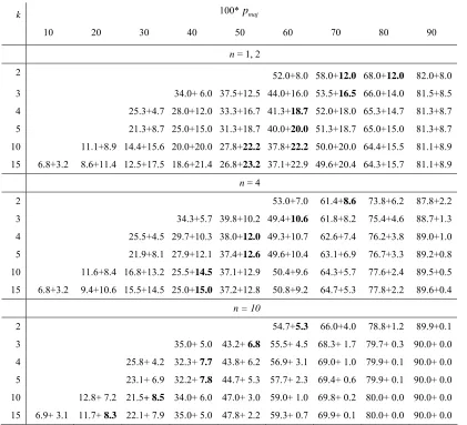
In Table 1, LCR and LSE for D pe( maj, )k are shown for n = 1, 2, 4 and 10 for several values of k and a range of values ofpmaj. For given n and k it is seen that, although LCR increases
very likely to be correctly determined and hence sampling error is low. Whenpmajis low, then the
consequence of wrongful determination of majority class, although more likely, is cushioned by the complimentary probability being only slightly less thanpmajand so loss of classification rate is
again minimal. As k and n increase, the maximum value of LSE tends to occur at smallerpmaj.
k 100*pmaj
10 20 30 40 50 60 70 80 90
n = 1, 2
2 52.0+8.0 58.0+12.0 68.0+12.0 82.0+8.0
3 34.0+ 6.0 37.5+12.5 44.0+16.0 53.5+16.5 66.0+14.0 81.5+8.5 4 25.3+4.7 28.0+12.0 33.3+16.7 41.3+18.7 52.0+18.0 65.3+14.7 81.3+8.7 5 21.3+8.7 25.0+15.0 31.3+18.7 40.0+20.0 51.3+18.7 65.0+15.0 81.3+8.7 10 11.1+8.9 14.4+15.6 20.0+20.0 27.8+22.2 37.8+22.2 50.0+20.0 64.4+15.5 81.1+8.9 15 6.8+3.2 8.6+11.4 12.5+17.5 18.6+21.4 26.8+23.2 37.1+22.9 49.6+20.4 64.3+15.7 81.1+8.9
n = 4
2 53.0+7.0 61.4+8.6 73.8+6.2 87.8+2.2
3 34.3+5.7 39.8+10.2 49.4+10.6 61.8+8.2 75.4+4.6 88.7+1.3
4 25.5+4.5 29.7+10.3 38.0+12.0 49.3+10.7 62.6+7.4 76.2+3.8 89.0+1.0
5 21.9+8.1 27.9+12.1 37.4+12.6 49.6+10.4 63.1+6.9 76.7+3.3 89.2+0.8
10 11.6+8.4 16.8+13.2 25.5+14.5 37.1+12.9 50.4+9.6 64.3+5.7 77.6+2.4 89.5+0.5
15 6.8+3.2 9.4+10.6 15.5+14.5 25.0+15.0 37.2+12.8 50.8+9.2 64.7+5.3 77.8+2.2 89.6+0.4
n = 10
2 54.7+5.3 66.0+4.0 78.8+1.2 89.9+0.1
3 35.0+ 5.0 43.2+ 6.8 55.5+ 4.5 68.3+ 1.7 79.7+ 0.3 90.0+ 0.0 4 25.8+ 4.2 32.3+ 7.7 43.8+ 6.2 56.9+ 3.1 69.0+ 1.0 79.9+ 0.1 90.0+ 0.0 5 23.1+ 6.9 32.2+ 7.8 44.7+ 5.3 57.7+ 2.3 69.4+ 0.6 79.9+ 0.1 90.0+ 0.0 10 12.8+ 7.2 21.5+ 8.5 34.0+ 6.0 47.0+ 3.0 59.0+ 1.0 69.8+ 0.2 80.0+ 0.0 90.0+ 0.0 15 6.9+ 3.1 11.7+ 8.3 22.1+ 7.9 35.0+ 5.0 47.8+ 2.2 59.3+ 0.7 69.9+ 0.1 80.0+ 0.0 90.0+ 0.0
Table 1: Leaf classification rate (LCR) and leaf sampling error (LSE) for leaf sample size n = 1,
2, 4 and 10 for various k andpmajunderD pe( maj, )k . Cell format is LCR + LSE, both
expressed as percentages; largest LSE for each k is shown bolded.
For k = 2, LSE reaches a maximum of approximately 12% when n = 1, 2 andpmajlies
between 0.7 and 0.8. For k > 2, LSE has the potential to be much larger than for k = 2 when n is
2 2
100 * ( maj (1- maj) /( -1))
LCR= p + p k
which decreases with k to100 *pmaj2. Thus, as k increases, LSE forD pe( maj, )k tends to
2
100 *pmaj −100 *pmaj = 100*pmaj(1−pmaj)
which has a maximum value of 25% atpmaj= 0.5. Table 1 shows that LSE can be 20% or above
for k≥ 5.
For n > 2 and givenpmaj, LCR forD pe( maj, )k can increase or decrease with k. This is because LCR, in Equation 5, is a convex combination of pmaj and (1-pmaj) /( -1))k weighted byPcorrand
1−Pcorr respectively. As k increases, Pcorrincreases and (1-pmaj) /( -1))k , which by definition is
less thanpmaj, decreases but its weight,1−Pcorr, is also decreasing.
Since the sampling error of the tree is the average of its leaf sampling errors, the behaviour of leaf sampling error should be reflected in the overall sampling error. As training set size increases, induced trees will tend to have more structure and so the leaf class probability distributions will be more informative with the result that individualpmajin the leaf distributions
will tend to increase. Thus the pattern of increase and decrease in sampling error with increases in
maj
p noted above for LSE should be observable in the sampling error for the whole tree.
5
The LED Domain Revisited
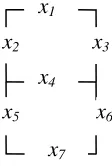
To illustrate the error decompositions described in Section 3 and to motivate further discussion, decompositions will be calculated for decision trees induced using training data generated from the LED artificial domain (Breiman et al., 1984). An LED display for digits has seven binary indicators as illustrated in Figure 1. Each of these is corrupted, that is, inverted, independently with a given probability. If each digit has the same prior probability of being selected for display, then a complete probability model on attributes (x1 , … , x7, class) has been defined. The class model can be derived and represented, extensionally, as a set of 128 rules whose conditions express the instantiation of (x1, …, x7) and associate this with a probability distribution on the vector of ten classes, (1, … , 9, 0).
Figure 1: Mapping of attributes in the LED display.
5.1 Experimental Results
Experiments to induce ID3 trees were carried out on data generated from the LED domain with corruption probability 0.1 for which the Bayes rate is 74.0%. These were repeated on the 24
x1 x4 x2 x3
x3
x1 x4 x2 x3
x3 x1 x2
x5 x4
attribute domain obtained by augmenting the seven attributes with 17 mutually independent binary pure noise attributes (Breiman et al., 1984). In a final series of experiments, random attribute selection was used for induction on the 24 attribute domain.
A number of replications were performed at each of several points along the learning curve varying from 10000 at sample size 25 down to 10 at sample size 10000. For each trial, the error decomposition in Equation 1 and the sub-decomposition of majority class error in Equation 2 were obtained yielding the overall decomposition in Equation 3.
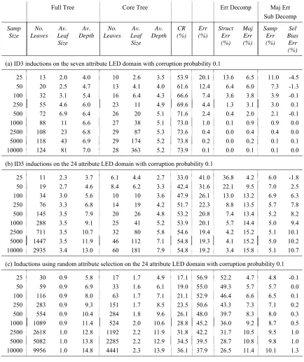
Sampling error was estimated in a tree by replacing each leaf with a freshly drawn random sample of the same size and obtaining the classification rate of the resulting tree. This produces an unbiased estimate of sampling error over replications and is more efficient than calculating the exact sampling error from the leaf class probability distribution, particularly when the sample reaching a leaf is large. The results are shown in Table 2.
For the seven attribute domain shown in Table 2(a), structure error decreases with sample size and is virtually eliminated at size 1000. For most of the learning curve, it is dominated by majority class error and the sub-decomposition shows that this is due mostly to sampling error with selection bias being either negative or approximately zero. Sampling error decreases with sample size due to the rapid increase in examples reaching the leaves. For sample sizes 25 and 50 the negative selection biases are two-tailed significant at the 5% level. The attribute selection competition here is aiding the determination of majority class: the sample reaching a leaf is better able to determine majority class than is an independent random sample.
Table 2 (b) shows that, with the addition of 17 pure noise attributes, the full trees are now much larger and that total error, structure and majority class error are considerably larger than for the seven attribute domain. There is still structure error at sample size 10000. Core trees are initially smaller but become larger as they inflate with locked in pure noise attributes. The large majority class error is due to both sampling and selection bias errors. Because of the availability of attributes for expansion, leaf sample sizes do not increase to reduce sampling error.
There is also some evidence of an increase and then decrease in sampling error due to a gradual increase in information in the leaf distributions as noted Section 4.2. In contrast to the seven attribute case, selection bias is now two-tailed significant at the 1% level along the learning curve apart from size 25, where, as for the seven attribute domain, it is significantly negative. As tree depth increases, there are fewer attributes available for selection, yet selection bias continues to increase along the learning curve suggesting that it accumulates with depth, that is, a leaf inherits a selection bias from its parent and adds to it.
Comparing Table 2 (c) with Table 2 (b) shows that random attribute selection produces much larger trees with fewer examples reaching each leaf. Core trees are also considerably inflated as is to be expected. The increase in error is accounted for by the much greater structure error. In contrast, the majority class error is generally much lower due to the reduction in selection bias error, which more than compensates for the larger sampling error. There is a modest increase in selection bias error along the learning curve becoming statistically different from zero at the 5% level from size 250 onwards. The process of tree expansion produces child node frequency configurations constrained to add up to that of the parent and which are, therefore, not genuinely independent of one another. Thus although there is no attribute selection competition, the process of repeatedly dividing a single overall sample into progressively smaller constrained sub-samples does produce a small bias.
Full Tree Core Tree Err Decomp Maj Err Sub Decomp
Samp Size
No. Leaves
Av. Leaf Size
Av. Depth
No. Leaves
Av. Leaf Size
Av. Depth
CR (%)
Err (%)
Struct Err (%)
Maj Err (%)
Samp Err (%)
Sel Bias
Err (%)
(a) ID3 inductions on the seven attribute LED domain with corruption probability 0.1
25 13 2.0 4.0 10 2.6 3.5 53.9 20.1 13.6 6.5 11.0 -4.5
50 20 2.5 4.7 13 4.1 4.0 61.6 12.4 6.4 6.0 7.3 -1.3
100 32 3.1 5.4 16 6.4 4.3 66.6 7.4 3.6 3.8 3.9 -0.1
250 55 4.6 6.0 23 11 4.9 69.6 4.4 1.3 3.1 3.0 0.1
500 72 6.9 6.4 26 20 5.1 71.6 2.4 0.4 2.0 2.1 -0.1
1000 88 11 6.6 27 38 5.1 73.0 1.0 0.1 0.9 0.9 0.0
2500 108 23 6.8 29 87 5.3 73.6 0.4 0.0 0.4 0.4 0.0
5000 118 43 6.9 29 174 5.2 73.8 0.2 0.0 0.2 0.1 0.1
10000 124 81 7.0 28 363 5.2 73.9 0.1 0.0 0.1 0.1 0.0
(b) ID3 inductions on the 24 attribute LED domain with corruption probability 0.1
25 11 2.3 3.7 6.1 4.4 2.7 33.0 41.0 36.8 4.2 6.0 -1.8
50 19 2.7 4.6 8.4 6.2 3.3 42.4 31.6 22.1 9.5 7.0 2.5
100 34 3.0 5.6 10 10 3.6 47.9 26.1 13.0 13.2 6.9 6.3
250 76 3.3 6.8 14 19 4.2 51.7 22.3 8.8 13.5 5.7 7.8
500 145 3.5 7.9 20 26 4.8 53.2 20.8 7.4 13.4 5.2 8.2 1000 288 3.5 9.1 25 41 5.2 53.9 20.1 5.7 14.4 5.0 9.4 2500 711 3.5 10.7 32 80 5.8 54.6 19.4 4.2 15.2 5.1 10.1
5000 1447 3.5 11.9 46 112 7.1 54.8 19.3 4.1 15.2 5.0 10.2
10000 2935 3.4 13.0 60 181 7.9 54.8 19.2 3.4 15.8 5.1 10.7
(c) Inductions using random attribute selection on the 24 attribute LED domain with corruption probability 0.1
25 30 0.9 5.8 17 1.7 4.9 17.1 56.9 52.2 4.7 4.8 -0.1
50 59 0.9 6.9 33 1.6 6.1 19.0 55.0 49.3 5.7 5.7 0.0
100 116 0.9 8.0 63 1.7 7.1 21.1 52.9 46.4 6.6 6.5 0.1 250 283 0.9 9.3 151 1.7 8.5 23.5 50.6 43.3 7.3 7.1 0.2 500 554 0.9 10.4 284 1.8 9.6 26.1 48.0 39.7 8.3 8.0 0.3 1000 1089 0.9 11.4 524 2.0 10.6 28.8 45.2 36.0 9.2 8.7 0.5 2500 2618 1.0 12.8 1192 2.2 11.9 31.8 42.2 31.7 10.5 9.5 1.0 5000 5082 1.0 13.8 2285 2.2 12.9 34.5 39.5 28.7 10.8 9.8 1.0 10000 9956 1.0 14.8 4441 2.3 13.9 36.1 37.9 26.5 11.4 10.1 1.3
Table 2: Tree statistics (No. Leaves = number of leaves in the tree; Av. Leaf Size = average
number of examples in the leaves of the tree; Av. Depth = average depth of the tree),
classification rate (CR), inductive error (Err) and error decompositions for tree
6
Experiments with the Autouniv Classification Model Generator
It is important to establish the extent to which the results from the LED domain, regarding the behaviour of the error decompositions, hold in general and how they change under different model characteristics. To investigate this, an artificial model generator, Autouniv, was built.
6.1 An Outline of the Autouniv Procedure
Autouniv produces a class model together with a joint distribution of the description attributes. At present the generator is implemented for discrete attributes only. To create a model, the number of informative attributes, pure noise attributes and classes are specified; the number of values for an attribute is specified as either a range across attributes or as the same fixed value for all attributes.
To create the joint attribute distribution, attributes are separated randomly into independent factors with the maximum number of attributes allowable in a factor also being specified. A pure noise attribute cannot be in the same factor as an informative attribute. The joint probability distribution for each factor is then generated at random. If the number of values for the attributes was specified as a range then, for each attribute, the actual number is randomized separately within this range.
To create the class model, a decision tree is generated and a class distribution is built at each leaf. The tree is then converted to a rule set. The tree is built in a random fashion as follows. At each expansion, an available attribute is selected at random from one of the informative factors. Pure noise attributes are never used for expansion. A minimum depth for the tree is set. After the tree has been built to this depth, further expansion along a path is controlled by a stopping probability, which is chosen at random between specified lower and upper limits and is generated independently at each leaf. This probability is then used in a ‘coin toss’ to determine whether the current node will be expanded. Finally, lower and upper limits are specified for the number of leaves of the tree. A tree will be rejected if its size is outside these limits. It will also be rejected if there is an informative factor at least one of whose attributes does not appear in the tree.
The class distribution at a leaf is created in two stages. First the majority class is selected from a specified distribution; ties are possible. Then the probability of this majority class (classes) is determined at random between given limits; these limits can be set differently for different classes. For the remaining non-majority classes, a subset of these is selected at random to receive positive probability which is assigned randomly.
The Autouniv procedure was developed to facilitate simple construction of a rich variety of realistic models. The tree building mechanism permits a degree of control of model complexity through specification of the number of informative attributes, the minimum depth of the tree, stopping probability range and the number of leaves. It also guarantees that all attributes declared as informative will be informative but also, through the factoring mechanism, that some of these may be redundant (Hickey, 1996). The procedure for constructing class distributions allows for specification of noise at different levels (and hence differing Bayes rates). It also permits heterogeneity in the noise across rules within a particular model. Some classes can be made noisier than others and class base rates can vary with one or more classes made rare if required.
In spite of the control provided by the parameters, some of the properties of the generated model remain implicit. An example is the degree of interaction of the description attributes. In some models most of the information about class will be carried by a small number of attributes whereas in others it will be distributed across a large number with no one or two attributes dominating.
to suppose that it might be biased towards creating models for which induced trees exhibit a particular pattern of error decomposition, such as unusually large majority class error.
Once it has been generated, a model can be queried for a supply of training examples: an example description is obtained randomly from the attribute joint distribution, the matching rule is looked up and a class determined using the class distribution for that rule.
Finally, the parameters settings can themselves be randomized between given limits. This allows for easy generation of a heterogeneous series of models for experimentation.
6.2 Experiments with Autouniv
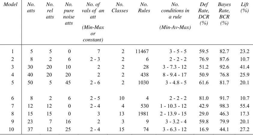
Ten models were generated to give variety with regard to the number of attributes and classes, default classification rate, lift, noise levels and model complexity. A summary of the main characteristics of these models is given in Table 3. All but three have pure noise attributes. The first five models have two classes; the remaining five have more than two classes. The columns headed No. Rules and No. conditions in a rule give an indication of model complexity. Most
models are heterogeneous in the lengths of rule conditions.
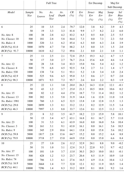
Experiments similar to those performed on the LED domains in Section 5 were carried out on these 10 models. The results are shown in Table 4 (for the first five models) and in Table 5 (for the remaining five). The principal model characteristics from Table 3 are summarized in the first columns of Tables 4 and 5 for convenience. A classification rate (CR) which is less than the
default classification rate (DCR) for the model is shown in italics in Tables 4 and 5. For several
models the classification rate remains below the default well into the learning curve indicating that interaction of several attributes is required for lift.
For all models, structure error falls along the learning curve and for most is almost eliminated by size 10000. The exception is model 4. From Table 3, model 4 is quite complex in that the minimum rule condition length is 8, which is greater than for the other models. Majority class error is substantial for all models and, for most, exceeds structure error in the latter part of the learning curve, remaining high even when structure error has almost been eliminated.
Model No. atts
No. rel atts
No. pure noise atts
No. of vals of an
att
(Min-Max or constant)
No. Classes
No. Rules
No. conditions in
a rule
(Min-Av-Max) Def Rate, DCR (%)
Bayes Rate, BCR (%)
Lift (%)
1 5 5 0 7 2 11467 3 - 5 - 5 59.5 82.7 23.2
2 8 2 6 2 - 3 2 6 2 - 2 - 2 76.9 87.6 10.7
3 30 20 10 2 2 28 3 - 7.3 - 12 51.2 92.6 41.4
4 40 20 20 2 2 438 8 - 9.4 - 17 50.9 76.8 25.9
5 50 5 45 2 - 6 2 1030 3 - 4.8 - 5 61.6 81.7 20.1
6 8 2 6 2 - 5 10 4 2 - 2 - 2 81.0 91.7 10.7
7 12 12 0 2 - 4 4 530 1 - 10.3 - 12 42.9 98.3 55.4
8 15 15 0 3 13 1981 2 - 13.9 - 15 29.0 46.3 17.3
9 23 7 16 2 3 9 3 - 3.2 - 4 59.8 79.9 20.1
10 37 12 25 2 - 4 15 74 3 - 6.3 - 12 16.9 44.1 27.2
Full Tree Err Decomp Maj Err Sub Decomp
Model Sample Size No. Leaves Av. Leaf Size Av. Depth CR (%) Err (%) Struct Err (%) Maj Err (%) Samp Err (%) Sel Bias Err (%)
25 34 0.8 2.1 52.3 30.4 23.0 7.4 7.2 0.2
50 67 0.8 2.5 52.7 30.0 22.6 7.4 7.7 -0.3
100 139 0.7 2.9 53.4 29.3 21.8 7.5 7.4 0.1
500 716 0.7 3.8 56.5 26.2 18.0 8.2 8.9 -0.7
1000 1435 0.7 4.2 57.7 25.0 15.5 9.5 9.8 -0.3
5000 5161 1.0 4.7 66.6 16.1 5.4 10.7 10.4 0.3
1
No. Atts: 5 No. Classes: 2 No. Rules: 11467 DCR (%): 59.5
BCR (%): 82.7 10000 7482 1.3 4.8 70.8 11.9 2.6 9.3 9.1 0.2
25 9 3.1 2.8 74.9 12.7 2.9 9.8 5.0 4.8
50 16 3.3 3.6 76.5 11.1 1.4 9.7 4.1 5.6
100 33 3.1 4.7 77.9 9.7 0.5 9.2 3.5 5.7
500 129 3.9 6.4 81.1 6.5 0.0 6.5 3.1 3.4
1000 206 4.9 6.8 82.8 4.8 0.0 4.8 2.4 2.4
5000 455 11.0 7.5 86.4 1.2 0.0 1.2 0.8 0.4
2
No. Atts: 8 No. Classes: 2 No. Rules: 6 DCR (%): 76.9
BCR (%): 87.6 10000 573 17.5 7.7 87.1 0.5 0.0 0.5 0.3 0.2
25 7 3.7 3.2 64.4 28.2 22.3 5.9 4.3 1.6
50 12 4.5 4.2 71.3 21.3 13.2 8.1 4.0 4.1
100 20 5.3 5.1 78.4 14.2 5.8 8.4 1.9 6.5
500 78 6.5 7.9 82.5 10.1 1.5 8.6 1.6 7.0
1000 149 6.8 9.5 83.7 8.9 1.0 7.9 1.6 6.3
5000 760 6.6 12.6 84.0 8.6 0.4 8.2 1.2 7.0
3
No. Atts: 30 No. Classes: 2 No. Rules: 28 DCR (%): 51.2
BCR (%): 92.6 10000 1588 6.3 14.4 84.4 8.2 0.1 8.1 1.1 7.0
25 7 3.5 3.3 50.2 26.6 25.4 1.2 1.4 -0.2
50 14 3.5 4.4 50.3 26.5 25.0 1.5 1.7 -0.2
100 28 3.6 5.5 50.4 26.4 24.8 1.6 1.8 -0.2
500 144 3.5 8.1 50.9 25.9 23.5 2.4 3.0 -0.6
1000 291 3.5 9.2 51.0 25.8 23.0 2.8 2.8 0.0
5000 1427 3.5 11.6 54.1 22.7 16.8 5.9 5.0 0.9 4
No. Atts: 40 No. Classes: 2 No. Rules: 438 DCR (%): 50.9
BCR (%): 76.8 10000 2846 3.5 12.7 55.3 21.5 14.6 6.9 5.0 1.9
25 18 1.5 1.9 53.9 27.8 20.0 7.8 6.6 1.2
50 33 1.6 2.4 54.2 27.5 19.7 7.8 7.1 0.7
100 66 1.5 2.8 54.1 27.6 19.4 8.2 7.0 1.2
500 309 1.6 3.9 56.9 24.8 15.7 9.1 7.3 1.8
1000 607 1.7 4.6 60.2 21.5 12.1 9.4 7.0 2.4
5000 2680 1.9 5.5 65.6 16.1 4.6 11.5 7.4 4.1
5
No. Atts: 50 No. Classes: 2 No. Rules: 1030 DCR (%): 61.6
BCR (%): 81.7 10000 5133 2.0 6.1 66.4 15.3 3.0 12.3 7.8 4.5
Full Tree Err Decomp Maj Err Sub Decomp
Model Sample Size No. Leaves Av. Leaf Size Av. Depth CR (%) Err (%) Struct Err (%) Maj Err (%) Samp Err (%) Sel Bias Err (%)
25 10 3.5 2.4 79.7 12.0 3.8 8.2 3.9 4.3
50 19 3.3 3.3 81.8 9.9 1.7 8.2 2.2 6.0
100 38 2.8 4.2 83.2 8.5 0.5 8.0 2.5 5.5
500 181 2.8 5.8 84.4 7.3 0.0 7.3 2.3 5.0
1000 320 3.1 6.2 85.4 6.3 0.0 6.3 2.4 3.9
5000 1070 4.7 7.0 88.2 3.5 0.0 3.5 1.5 2.0
6
No. Atts: 8 No. Classes: 10 No. Rules: 4 DCR (%): 81.0
BCR (%): 91.7 10000 1610 6.2 7.2 89.6 2.1 0.0 2.1 1.0 1.1
25 11 2.5 2.1 72.8 25.5 19.3 6.2 4.7 1.5
50 17 3.0 2.7 76.7 21.6 15.6 6.0 4.6 1.4
100 28 3.8 3.4 83.3 15.0 9.6 5.4 4.2 1.2
500 75 6.8 4.5 92.5 5.8 2.7 3.1 1.4 1.7
1000 138 7.4 5.1 93.1 5.2 1.8 3.4 1.0 2.4
5000 525 9.6 6.5 95.0 3.3 0.6 2.7 0.7 2.0
7
No. Atts: 12 No. Classes: 4 No. Rules: 530 DCR (%): 42.9
BCR (%): 98.3 10000 1071 9.3 7.3 95.7 2.6 0.4 2.2 0.3 1.9
25 22 1.1 3.0 20.0 26.3 14.3 12.0 12.1 -0.1
50 43 1.2 3.7 25.0 21.3 10.5 10.8 10.6 0.2
100 82 1.2 4.4 27.6 18.7 7.3 11.4 10.2 1.2
500 382 1.3 5.8 31.9 14.4 1.6 12.8 11.0 1.8
1000 760 1.3 6.5 32.5 13.8 1.0 12.8 11.5 1.3
5000 3899 1.3 8.1 33.2 13.1 0.2 12.9 11.5 1.4
8
No. Atts: 15 No. Classes: 13 No. Rules: 1981 DCR (%): 29.0
BCR (%): 46.3 10000 7997 1.3 8.8 33.7 12.6 0.1 12.5 11.2 1.3
25 8 3.2 3.5 61.7 18.2 2.3 15.9 5.8 10.1
50 15 3.4 4.7 63.1 16.8 0.1 16.7 5.7 11.0
100 31 3.3 6.1 63.9 16.0 0.0 16.0 5.6 10.4
500 161 3.1 9.1 63.8 16.1 0.0 16.1 5.6 10.5
1000 345 2.9 10.6 64.1 15.8 0.0 15.8 5.6 10.2
5000 1817 2.8 13.6 64.7 15.2 0.0 15.2 6.4 8.8
9
No. Atts: 23 No. Classes: 3 No. Rules: 9 DCR (%): 59.8
BCR (%): 79.9 10000 3718 2.7 15.0 64.9 15.0 0.0 15.0 6.6 8.4
25 27 1.0 2.6 11.2 32.9 24.1 8.8 9.0 -0.2
50 51 1.0 3.1 12.6 31.5 22.0 9.5 9.7 -0.2
100 101 1.0 3.7 13.8 30.3 20.3 10.0 10.1 -0.1
500 428 1.2 5.3 23.7 20.4 8.5 11.9 10.9 1.0
1000 786 1.3 6.1 27.6 16.5 4.9 11.6 10.4 1.2
5000 3664 1.4 7.7 32.0 12.1 0.2 11.9 10.5 1.4
10
No. Atts: 37 No. Classes: 15 No. Rules: 74 DCR (%): 16.9
BCR (%): 44.1 10000 7296 1.4 8.3 33.2 10.9 0.1 10.8 9.2 1.6
Sampling errors are consistent with those expected from the discussion in Section 4.2 and from Table 1. In model 4, which has the lowest initial sampling error, the default rate is 50.9% indicating that near the beginning of the learning curve there is little penalty from obtaining an incorrect majority class. As the trees acquire structure, sampling error rises while the sample size at the leaf remains constant. The largest sampling error occurs for models 8 and 10, which have 13 and 15 classes respectively and quite low default and Bayes rates. Leaf sample sizes are smallest for these models. Sampling errors, though, fall short of the maxima in Table 1.
Selection bias error shows a more complex pattern. There are instances of very high bias and of virtually non-existent bias and the extent seems comparatively unrelated to the number of attributes and other characteristics of the model. For model 1 with five attributes, it is similar to that seen for the seven attribute LED domain. For model 2, however, with eight attributes, it is fairly large at the beginning of the learning curve when the leaf sample size is small, falling later on when it increases. In contrast, for model 4, with 40 attributes, 20 of which are pure noise, selection bias error only becomes statistically significant from size 5000.
There is some indication that the occurrence of larger selection bias is associated with simpler models such as 2, 3, 6 and 9. A possible explanation for this is that when structure error is low, the attribute selection competition is taking place amongst attributes none of which can offer much information gain. The competition is then more vulnerable to spurious leaf distributions.
6.2.1 R
ANDOMT
REESAll experiments were repeated with random attribute selection. The random trees were much larger for all models, typically having between 2 and 4 times as many leaves as the corresponding ID3 trees. For all models, except model 1, the classification rates along the learning curve were significantly lower than for the corresponding ID3 curve.
The random trees for model 1 matched the classification rates for ID3, with no significant difference all along the learning curve. Likewise there was no significant difference in decomposition errors. This is due to there being only five attributes all of which are relevant. Moreover, from Table 4, the classification rates are less than the default until after sample size 1000 so that the lift is shared amongst the attributes rather than being concentrated in one or two. Thus, as noted by Liu and White (1994), there is little benefit from selection based on maximising information gain over that offered by random selection.
For nearly all models, the selection bias error was virtually eliminated along the learning curve. Only for models 6 and 9 was here a slight increase as was observed for the LED domain.
These results broadly confirm the findings of Liu and White (1994). Their poorer performance is due to much larger structure error caused by the interference of pure noise attributes. They tend to have very much larger reduced cores indicating a high degree of inflation. Where the ID3 tree has significant selection bias error, this will be almost eliminated in the random tree but this benefit, which may be accompanied anyway by larger sampling error due to smaller leaf samples, is usually not sufficient to compensate for the increased structure error.
7
Experiments with Real Data
In the Forest Cover data, seven species of tree are classified using 54 attributes that describe their location. The data consists of 581012 examples. There are no missing values. Five of the classes are comparatively rare. These were combined into a single class called ‘other’. There are 40 binary attributes that describe soil type. These were eliminated. Four binary attributes describing wilderness area were combined into a single four-valued wilderness attribute.
The remaining 10 attributes are all continuous. These were made discrete by binning each into four bins with labels 1, 2, 3 and 4 as shown in Table 6.
Attribute Binning Ranges for Bins 1 - 4
1 2 3 4
Elevation < 2400 2400 < 3000 3000 < 3300 ≥ 3300 Aspect < 60 60 < 180 180 < 300 ≥ 300 Slope < 11 11 < 33 33 < 55 ≥ 55 Horizontal_Distance_To_Hydrology < 233 233 < 699 699 < 1165 ≥ 1165 Vertical_Distance_To_Hydrology < -44 -44 < 214 214 <472 ≥ 472 Horizontal_Distance_To_Roadways < 1187 1187 < 3559 3559 < 5930 ≥ 5930 Hillshade_9am < 42.3 42.3 < 127.0 127.0 < 211.7 ≥ 211.7 Hillshade_Noon < 42.3 42.3 < 127.0 127.0 < 211.7 ≥ 211.7 Hillshade_3pm < 42.3 42.3 < 127.0 127.0 < 211.7 ≥ 211.7 Horizontal_Distance_To_Fire_Points < 1196 1196 < 3587 3587 < 5978 ≥ 5978
Table 6: Continuous to discrete conversion of 10 Forest Cover attributes.
The final data set consists of 11 discrete attributes and three classes. This was split randomly into approximately 75% to represent the model and 25% to be used as a test set. Statistics relating to these sets are shown in Table 7.
Class Distribution
Data Set Size Lodgepole Pine Spruce/Fir Other
Whole 581012 (100%)
283301 (48.76%)
211840 (36.46%)
85871 (14.78%) Model 436169
(75.1%)
212587 (48.74%)
158968 (36.45%)
64614 (14.81%) Test 144843
(24.9%)
70714 (48.82%)
52872 (36.50%)
21257 (14.68%)
Table 7: Statistics for the revised Forest Cover data with 11 attributes and three classes obtained from a random partitioning into model and test subsets.
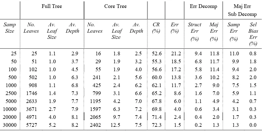
the 1 standard error setting was applied. The resulting tree, which is an approximation to the true model, had 1131 leaves. The rule set derived from this tree was applied to the test set producing a classification rate of 73.78% as an estimate of the true Bayes rate. From Table 7, the default classification rate in the test set is 48.82% giving a lift of 24.96%.
Experiments similar to those in Sections 5 and 6 were carried out on the revised data. Training examples were drawn randomly from the model data set. To determine structure and majority class error, an estimate of the true majority class at a leaf in an induced tree needs to be obtained. This was provided by applying the rule condition associated with the leaf to the whole of the model data set. The majority class amongst examples matching this condition was then taken as the estimate of the true majority class. Such estimates are typically based on fairly large numbers of matching examples. For example, if a tree induced from 10000 examples has a leaf containing two examples then the expectation, from Table 7, is that there would be 2 * 436169/10000 = 87 matching examples in the model set. These estimates of majority class were also used to estimate the reduced core of each induced tree through same majority class pruning.
Sampling error was calculated by the method described in Section 5 using random samples obtained from the model data set. All classification rates needed for the decomposition were estimated from the test data set.
The results, shown in Table 8, exhibit similar patterns of decomposition to those seen earlier. A sample of about 30000 is required to virtually eliminate structure error. Majority class error dominates structure error all along the learning curve. This is mostly due to sampling error. The low selection bias error across the learning curve is consistent with that observed for the more complex artificial models in Section 6.
Full Tree Core Tree Err Decomp Maj Err
Sub Decomp
Samp Size
No. Leaves
Av. Leaf Size
Av. Depth
No. Leaves
Av. Leaf
Size Av. Depth
CR (%)
Err (%)
Struct Err (%)
Maj Err (%)
Samp Err (%)
Sel Bias
Err (%)
25 25 1.1 2.9 16 1.8 2.5 52.6 21.2 9.4 11.8 11.0 0.8
50 51 1.0 3.7 29 1.9 3.2 55.3 18.5 6.8 11.7 9.9 1.8
100 102 1.0 4.5 55 1.9 4.0 56.6 17.2 5.8 11.4 9.4 2.0 500 502 1.0 6.3 241 2.1 5.6 60.0 13.8 3.6 10.2 8.2 2.0 1000 908 1.1 6.8 425 2.4 6.2 62.1 11.7 2.7 9.0 7.5 1.5
2500 1746 1.4 7.3 799 3.1 6.6 65.2 8.6 1.6 7.0 5.9 1.1
5000 2633 1.9 7.7 1195 4.2 7.0 67.8 6.0 1.1 4.9 4.2 0.7
10000 3671 2.7 7.9 1597 6.3 7.2 69.8 4.0 0.6 3.4 3.1 0.3
20000 4971 4.0 8.1 2065 9.7 7.4 71.4 2.4 0.4 2.0 1.7 0.3
30000 5727 5.2 8.2 2402 12.5 7.5 72.3 1.5 0.2 1.3 1.3 0.0
8
Conclusion and Future Work
The contribution of this paper has been the introduction of a method of decomposition of the classification error occurring in decision tree induction. Its application has been demonstrated on both artificial and real data. Instead of comparing tree induction algorithms in terms of classification error is it now possible to provide further insight into how this arose, specifically whether it is due to failure to grow sufficient tree structure or to successfully estimate majority class at the leaves.
It has been shown that majority class error is often quite substantial and that it can be further broken down into sampling error and selection bias error with the extent of these sources being quantified.
By factoring out the effects of selection bias, the sub-decomposition of majority class error permits a statistical analysis of sampling error not previously possible because of the biased samples reaching the leaves. For two classes, sampling error appears to be limited to a maximum of about 12%. For more than two classes it could be as much as 25%. Sampling error does decrease reasonably quickly when the size of sample reaching the leaves eventually begins to increase, particularly if the level of noise in the domain is low.
In ID3, selection bias error is due to the corruption in the sample reaching a leaf caused by the multiple comparison effect of the competition to select the best attribute with which to expand the tree. It may be insignificantly different from zero along the learning curve even when there are a large number of attributes involved in the selection competition and yet may be large when there are only a small number of attributes. The initial evidence provided here supports the hypothesis that if the underlying model is sufficiently complex, then this offers some protection against selection bias error. Although regarded here as a source of majority class error, selection bias error could, conceivably, be viewed as part of the error in forming tree structure.
The results provided here offer further insight into why ID3 typically outperforms trees grown with random attribute selection. It is due to a largely successful trade-off in forming structure efficiently at the expense of creating selection bias error.
The challenge for future work is to use the decomposition to develop better tree induction algorithms. For example, it may be possible to find a better trade-off between forming structure and incurring selection bias than that offered by ID3. The decomposition can be applied to induced trees however constructed. In particular, it can be obtained for trees that have been pruned and so should enhance investigation into issues relating to overfitting avoidance (Schaffer, 1993) and the properties of methods of pruning (Oates and Jensen, 1997; 1999).
It may also be possible to extend the approach to investigate the behaviour of bagging and boosting techniques for decision trees.
Majority class error was decomposed into sampling and selection bias errors. It is possible, instead, to decompose it in a way that reflects contributions from the reduced core and from extension beyond the core. Such an alternative sub-decomposition may be especially useful in investigating overfitting avoidance. Structure error can also be decomposed to isolate the effect of pure noise attributes on the induction. Work is being undertaken on both of these.
References
Robert E. Bechhofer, Salah Elmaghraby and Norman Morse. A single sample multiple-decision procedure for selecting the multinomial event which has the highest probability. Annals of Mathematical Statistics, 30:102-119, 1959.
Eibe Frank. Pruning Decision Trees and Lists. PhD thesis, University of Waikato, Hamilton,
New Zealand, 2000.
Carlos R.P. Hartmann, Pramod K. Varshney, Kishan G. Mehrotra and Carl L. Gerberich. Application of information theory to the construction of efficient decision trees. IEEE Transactions on Information Theory, IT-28:565-577, 1982.
Ray J. Hickey. Artificial universes: towards a systematic approach to evaluating algorithms which learn from examples. In Proceedings of the Ninth International Conference on Machine Learning, pages 196-205, Aberdeen, Scotland, 1992.
Ray J. Hickey. Noise modelling and evaluating learning from examples. Artificial Intelligence,
82(1-2):157-179, 1996.
Gareth M. James. Variance and bias for general loss functions. Machine Learning,
51(2):115-135, 2003.
David D. Jensen and Paul R. Cohen. Multiple comparisons in induction algorithms. Machine Learning, 38(3):309-338, 2000.
Harry Kesten and Norman Morse. A property of the multinomial distribution. Annals of Mathematical Statistics, 30:120-127, 1959.
Ron Kohavi and George H. John. Wrappers for feature subset selection. Artificial Intelligence,
97(1-2):273-324, 1997.
Wei Zhong Liu and Allan P. White. The importance of attribute selection measures in decision tree induction. Machine Learning,15(1):25-41, 1994.
Albert W. Marshall and Ingram Olkin. Inequalities: The Theory of Majorisation and its Applications. Academic Press, New York, 1979.
Tom M. Mitchell. Machine Learning. McGraw-Hill, New York, 1997.
Tim Oates and David D. Jensen. The effects of training set size on decision tree complexity. In
Proceedings of the Fourteenth International Conference on Machine Learning, pages. 254-261,
Nashville, Tennessee, 1997.
Tim Oates and David D. Jensen. Toward a theoretical understanding of why and when decision tree pruning algorithms fail. In Proceedings of the Sixteenth National Conference on Artificial Intelligence, pages 372-378, Orlando, Florida, 1999.
Foster Provost and Pedro Domingos. Tree induction for probability-based ranking. Machine Learning, 52(3):199-215, 2003.
J. Ross Quinlan. Induction of decision trees. Machine Learning,1(1):81-106, 1986.
Cullen Schaffer. Overfitting avoidance as bias. Machine Learning, 10(2):153-178, 1993.
Gary M. Weiss and Haym Hirsh. A quantitative study of small disjuncts. In Proceedings of the Seventeenth National Conference on Artificial Intelligence, pages 665-670, Austin, Texas,