The General Analytical and Numerical Solution for the Nonlinear Klein-Gordon Equation

(1)

The General Analytical and Numerical Solution for the

Nonlinear Klein-Gordon Equation

K. Karimi

Department of Mathematics, Imam Khomeini International University,

Qazvin, Iran

D. Rostamy

Department of Mathematics, Imam Khomeini International University,

Qazvin, Iran

N. Khodayar Department of Computer, Roudehen Branch, Islamic Azad

University, Roudehen, Iran

Abstract – We investigate the analytical solutions of the nonlinear Klein-Gordon equation with cubic nonlinearity, by applying the idea of commutative hypercomplexmathematics. And also, we apply Bernstein Spectral method to approx-imate the solution of the nonlinear Klein-Gordon equation. Illustrative example is included to demonstrate the validity and applicability of the technique.

Keywords – Nonlinear Klein-Gordon Equation, Commuta-tive Hypercomplexatematics, Bernstein Polynomials, Colloca-tion.

I. I

NTRODUCTION

In nuclear and high energy physics the study of exact solution of the Klein-Gordon equation is of high impor-tance for mixed scalar and vector potentials. However, the problem of exact solution of the Klein-Gordon for a num-ber of special potential has been of great interests in the recent years. The Klein-Gordon equation plays an impor-tant role in mathematical physics [1, 2]. The equation has attracted much attention in studying solutions and con-densed matter physics [3], in investigating the interaction of solutions in a collision less plasma, the recurrence of initial states, and in examining the nonlinear wave equa-tions [4]. Different techniques have been assumed by dif-ferent authors to obtain the exact solution of the Klein-Gordon with some typical potential. [5, 6, 7, 8, 9, 10]. The study of numerical solutions of the Klein Gordon and sine-Gordon equations has been investigated considerably in the last few years. [11, 12, 13, 14, 15]. In this paper we are dealing with the numerical approximation of the following nonlinear Klein-Gordon equation with cubic nonlinearity

utt+ αuxx + βu + γu3= f x, t , (1)

Where α, β andγ are known constant. In the present pa-per Bernstein polynomialsand Bernstein opa-perational ma-trix is presented. In this approach, a truncated Bernstein series together with the Bernstein operational matrix are used to convert problem to a system of linear algebraic equations. We demonstrate the relation between the Bernstein and Legendre polynomials. By using this rela-tion we derive the operarela-tional matrices of derivative of Bernstein polynomials. Then we employ them for solving our problem. The remainder of this paper is organized as follows. In Section 2, we give an overview of Bernstein polynomials, and relevant properties of commutative hypercomplex mathematics that needed in the sequel. In Section 3, by using the commutative hypercomplex ma-thematics we obtain Analytic solutions of the nonlinear Klein-Gordon equation. In Section 4, we making Bernstein operational matrix and also we apply Bernstein Spectral

method in section 5. Finally, Section 6 gives numerical result exhibiting the accuracy and efficiency of our pro-posed numerical algorithms.

II. P

RELIMINARIES AND

N

OTATION

In the section, we give some properties of the Bernstein polynomials and also, we summarize the properties of the commutative hypercomplexmatrmatics.

A. Bernstein polynomials

Bernstein polynomials of degree m, on the interval [0, 1] as basis functions for the linear space of polynomials are defined as

Bi,m = (−1)k m−i

k=0

m i

m − i k x

i+k_{, (2)}

i=0,1,…,m

A polynomial h(x) of degree m canbe expressed as h x = bi

m

i=0

Bi,m = bTϕ x , (3)

where the Bernstein coefficient vector b and the Bernstein vector ∅(x) are given by

bT= b0, b1, … , bm , (4)

and

ϕ x = [B0,m x , B1,m x , … , Bm,m x (5)

The product of Bernstein polynomials is

Bi,m x Bi,n x = m

i m

j m +n

i+j

Bi+j,m+n x , (6)

and

Bi,m x dx = 1 m+1 1

0 (7)

For details, see [16].

The Legendre polynomials constitute an orthonormal basis on the interval [0, 1],we define as follows

L0 x = 1, L1 x = 2x− 1,

Li+1 x =

2i + 1 2x − 1 i + 1 Li x −

i

i + 1Li−1 x ,

i=1, 2,…

The analytic form of the shifted Legendre polynomial Li(x) of degree i given by

Li(x) = −1 (i+k) i+k !x

k

i−k !k!2

i

k=0 .

Note that Li(0) = (−1)i andLi(1)= 1. The orthogonality condition is

Li x Lj 1

0

x dx =

0, for i ≠ j, 1

2i + 1, for i = j.

(2)

Pm x = ljLj x = lTφ x , m

j=0

(8)

Where the shifted Legendre coefficient vector l and the shifted Legendre vector φ(x)are given by

lT _{= l}

0, … lm ,

φ x = [L0 x , L1 x , … Lm x ]T 9

The derivative of the vector φ(x) can be expressed by

dφ x

dx = Dlφ x (10)

where matrix Dl is the (m + 1) × (m + 1) operational ma-trix of derivative of theshifted Legendre polynomials on the interval [0,1] given by

Dl = di+1,j+1=

2 2j + 1 , for j = i − k, 0, for otherwise. k = 1,3, … m, if m odd, k = 1,3, … , m − 1, if m even,

B. Commutative hypercomplex mathematics

Systems of hypercomplex numbers, which had been studied and developed at the end of the 19th century, are nowadays quite unknown to the scientific community. Itis believed that study of their applications ended just before one of the fundamental discoveries of the 20th century, Einsteins equivalence between space and time. Owing to this equivalence not-defined quadratic forms have got concrete physical meaning and have been recently recog-nized to be in strong relationship with a system of bidi-mensional hypercomplex numbers. The commutative hypercomplex mathematics is an extension of complex numbers that obeys the axioms of the classical complex variables. It is 4-D independent variable, so we will use the notation Z = 1x + iy+jz + kct, where x, y, z, ct are real and Z belong to an element of the commutative hyper-complex algebra. In the fourth component, t represents time, and c is a scale factor [17].

Analytic function is defined as following:

F Z = F ξ e1+ F(η)e2,

ξ= x − ct + i y + z ,

η= x + ct + i y − z , e1=

1 − k

2 , e2= 1 + k

2 .

The 4-D function F(Z) is analytic if both F(ξ) and F(η) are analytic in the classical complex variable sense. Now, we introduce operators such as derivative and integral for functions of a 4-D variable. They obey the function defini-tion that we already have. Therefore, they are as follow-ing:

Open (Z) = oper (ξ)e1+ oper η e2.

The result is that we can apply all of the powerful tools of complex analysis tofour-space problems. The 4-D Cauchy-Riemann (C-R) conditions which have a number of interesting is:

dF dZ= 1

∂F ∂x= −i

∂F ∂y= −j

∂F ∂z= k

∂F

∂ct (11)

C-R conditions say that the derivative ofa 4-D analytic function is the same withina sign in all four coordinate directions. The first two equalities are the same asfor complex variables. These equations can be used to reduce a partial differential equation in several real, independent variables to an ordinary differential equation in one 4-D

variable. By doing so, we would be imposing continuity conditions on the PDE, because the C-R conditions are a statement of continuity. PDEs aretypically derived with the assumption of continuity, but without its explicit inclu-sion because convenient means have not been available. Note carefully that we are not constraining any potential solution, because the C-R conditions hold for any and all analytic functions.

III. A

NALYTIC

S

OLUTION OF THE

K

LEIN

-G

ORDON

E

QUATION

In this section we impose a proposition that says how to get the analytic solutions of the KleinGordon equation.

Proposition 3.1.

The general analytical solution of Eq.(1) in 4-D space is as following:

u x, ct = ± 2i b D +

βη2_{− Aα}

η2_{− A} (12)

Where,

η = Sn β − δ α − γ

4 3 x + kct − z0 ,

(β − γ)(α − δ) (α − γ)(β − δ)

A =β − δ α − δ.

In above, we have α, β, γ, δ,z0are the arbitrary constants, and k is a 4-D algebraicbasis element and c is a scale fac-tor.

Proof.

As mentioned previous section, our basic approach to solution is to first convert the (nonlinear) Klein-Gordon equation to an ODE, then solve it by means of classical methods. To convert partial differentials to ordinary deriv-atives, we shall use the 4-D Cauchy-Riemann equations (11), where Z = 1x + iy + jz + kct ([18]).

Making the partial derivative conversions, Eq.(1) converts to

k2_c2d 2_u

dZ2+ μ

d2_u

dZ2+ eu + au

3_{= 0 (13)}

By considering k2 = 1 we have:

c2_{+ μ}d 2_u

dZ2+ eu + au

3_{= 0 (14)}

This equation is still nonlinear, but is solvable by direct methods. We rearrange,multiplyboth sides of the equation by the first derivative and also let c2 + α= b, then integrate to get:

−b 2

du dz

2

=a 4u

4₊e

2u

2_{+ B, (15)}

The element B is another 4-D constant of integration. We consider above equation to polynomial in u. Ames ’s given the solution in this form in [19].

a 4u

4₊e

2u

2_{+ B =}a

4[u

4_{− α + β + γ + δ u}3₊

αβ + γδ + α + β γ + δ u2_{− [ α + β γδ +}

+(γ + δ)aβ]u + αβγδ]

Then, we see

α + β + γ + δ = 0, a

4 αβ + γδ + a + β γ + δ = c 2,

(3)

integration and we yield:

± 2bi

2 u Z = D +

(βη2_{− Aα)}

(η2_{− A)} ,

A =β − δ α − δ,

η = Sn (β − γ)(α − γ)

4 3 Z − z0 ,

(β − γ)(α − δ) (α − γ)(β − δ) .

The element D is the third 4-D constant of integration, z0 is arbitrary constant and the function Sn[...] is the Jaco-bi elliptic function. Above proposition gives us the general analytical solution for the KleinGordon equation in terms of the 4-D commutative hypercomplex variable Z. It is the complete solution for the ODE form in as much as we have integrated twice and have a solution including two arbitrary constants of integration.

We have obtained a solution u(Z) in terms of one varia-ble having three space dimensions and time. One question that must be answered is, “Does it reduce to a solution of the original, one-dimensional KleinGordon equation when the y, z components are set to zero?”, this is enough to check. Setting y = z = 0 and assuming that z0 is a constant in this space, we get:

u x, ct = ± 2i b[D +

(βη2_{− Aα)}

(η2_{− A)} (16)

Where, we have

η = Sn β − δ α − γ

4 3 x − Kct − z0 ,

(β − γ)(α − δ) (α − γ)(β − δ)

IV. O

PERATIONAL

M

ATRIX OF

D

IFFERENTIATION

In this section, we will try to derive an explicit formula for the (m+1)(m+1) matrix Db that is called operational matrix of derivative Bernstein polynomials. Firstly, we demonstrate the relation between the Bernstein and Le-gendre polynomials by introducing transformation matrix W and G. [20]. The Legendre polynomial Lk(x) can be expressed in the k − th degree Bernstein basis B0,k(x),B1,k(x), ...,Bk, k(x) as

Lk x = −1 k+i

k

i Bi,k x

k

i=0

(17)

Now consider a polynomial Pm(x) of degree m, ex-pressed in the m − th degree Bernstein and Legendre bases on x ∈ [0, 1] :

Pm x = cjBj,m x = m

j=0

lk m

k=0

Lk x (18)

We write the transformation of the Legendre polyno-mials on [0, 1] into the m –thdegree Bernstein basis func-tions as

Bk,m x = wk,iLi m

i=0

x , k = 0, … , m (19)

The elements wk,i,k,i = 0, 1, ...,m, form an (m+1)×(m+1) basis conversion matrix W. To compute them, we multiply Eq. (19) by Lj(x), integrate over x ∈ [0, 1], we have

wk,j = 2j + 1 Bk,m 1

0

x Lj x dx. (20)

We now replace Eq. (17) into (20) and obtain

wk,j = 2j + 1 −1 j+i j

i=0

k

i Bk,m

1

0

x Bi,j x dx.

The integrals of the products of Bernstein basis func-tions can be found using

1 − x r 1

0

xi_{dx =} 1

r + i + 1 r+i_i , r, i ∈ N ∪ 0 ,

As follows:

Bk,m 1

0

x Bi,j x dx =

m k

j i x

k+i_{(1 − x)}m+j−k−i 1

0

dx =

m k

j i

(m + j + 1) m+j_k+i

Therefore, we have the elements of W as

wk,j =

2j+ 1

m + j + 1 m

k −1

j+i j i

j i m+j k+i j

i=0

,

k, j = 0, … m.

Now, we write the transformation of the B-polynomials on [0, 1] into m-th degree

Legendre basis functions as

Lk x = Gk,j M

j=0

Bj,m x (21)

k = 0, … , m,

The elements Gk,j form an(m+1)×(m+1) basis conver-sion matrix G. ReplacingEq.(21) into Eq. (18) and re-arranging the order of summation, we obtain

cj= lkGk,j m

k=0

, j = 0, … , m (22)

Since we can express each k-th degree Bernstein basis function in the m-th degree Bernstein basis as

Bi,k= k

i m−k

j−i m

j m−k+i

j=i

Bj,m x , (23)

i = 0, … , m, i = 0, . . , k,

replacing Eq. (23) into Eq. (17) and re-arranging the order of summation, we find that the basis transformation (21) is defined by the elements

Gk,j=

1

m j

−1 k+j k

i

min j,k

i=r

k i

m − k j − i ,

r = max 0, j + k − m , (24)

of the matrix G for k, j = 0, ...,m. If we denote the Legen-dre basis vector as using Eqs. (5), (9), (19) and (21) we have

(4)

V. S

OLUTION OF THE

P

ROBLEM

Suppose ϕ(x) and ϕ(t) are vectors of Bernstein polyno-mials on [0,1] defined in Eq.(5). Now the unknown func-tion u(x, t) in Eq. (1) can be approximated as

u x, t ≃ ϕT_{x Uϕ t , (28)}

where the unknown matrix U is (m + 1) × (m + 1) and can be shown as

U1,1 ⋯ U1,m+1

⋮ ⋱ ⋮ Um+1,1 ⋯ Um+1,m+1

.

We can write

utt x, t = ϕ x T

UDb2ϕ t (29)

Also we have

uxx x, t = (Db2ϕ x )TUϕ t = ϕT x (Db2)TUϕ t (30)

Using Eqs. (28-30) in Eq. (1), we obtain

(ϕ(x))T_UD b

2_{ϕ t + αϕ}T_(x)(D b

2₎T_{Uϕ x}

+βϕT_{(x)Uϕ t}_{+ γ(ϕ}T _x_Uϕ _t ₎3_{= f} _{x, t} ₍₃₁₎

We now collocate Eq. (31) in (m−1)×(m−1) points (xi, tj), i = 2, ...,m, j = 2, ...,m, as

R xi, tj = (ϕ(xi))TUDb2ϕ tj αϕT(xi)(Db2)TUϕ tj

+βϕT_x

i Uϕ tj + γ(ϕT xi Uϕ tj )3= f xi,tj

(32) where xi, i = 1, ...,m+1, are shifted points of Lj on the [0, 1] and tj ,j = 1, ...,m+1, are the shifted points of Lj on [0, T] totally we can choose Chebyshev collocation points instead of Legendre collocation points. [21]. Collocating initial and boundary condition in m+ 1 points xi, i = 1, ..., m+ 1, and m points tj , j = 1, ...,m, we gain

u 0, tj = f1 tj , u 1, tj = f2 tj (33)

j = 2, … . , m ,

u xi, 0 = g xi , (34)

i = 1, … , m + 1.

ut xi, 0 = h xi , 35)

i = 1, … , m + 1.

Hence we observe that Eq. (32) together with Eqs. (33, 34) and (35) produce asystem of equations, which can be solved for the unknown Ui,j . In next section, we give some results of numerical experiments with methods based on the preceding sections.

VI. N

UMERICAL

R

ESULT

In this section, for testing the accuracy and efficiency of described method we solvefollowing nonlinear example. For this aim, we consider the nonlinear Klein-Gordonequation (1) with cubic nonlinearity with con-stants, α =−2.5, β = 1 and γ = 1.5 in the interval (x, t)∈ [0, 1] × [0, 1]. The initial conditions are given by

u x, 0 = Btan Kx , x ∈ 0,1 ut x, 0

= BcKsec2_{Kx , x ∈ 0,1 ,}

and the exact solution by [22] is

u x, t = Btan K x + ct ,

Where B= β

γ and K = −β 2(α+c2₎.

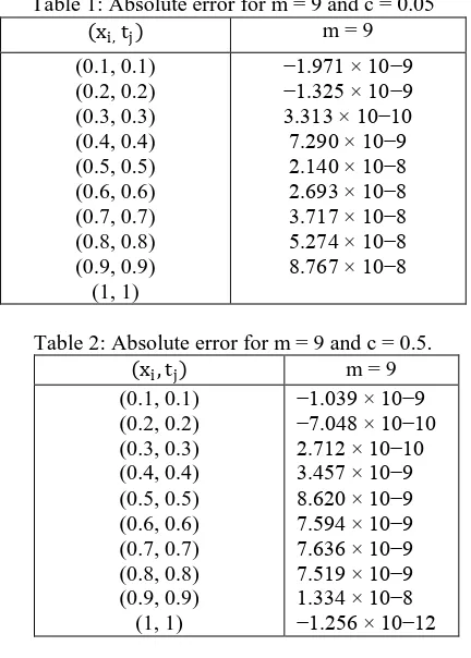
In this example f(x, t) = 0. We extract the boundary function from the exact solution. The obtained numerical results by means of the proposed method are shown in Table 1. In Table 1 and In Table 2 we compare the exact solution and approximate solution by our method for m = 9, c = 0.05 and c = 0.5. The presented results,show the efficiency and accuracy of the method.

Table 1: Absolute error for m = 9 and c = 0.05

(xi, tj) m = 9

(0.1, 0.1) (0.2, 0.2) (0.3, 0.3) (0.4, 0.4) (0.5, 0.5) (0.6, 0.6) (0.7, 0.7) (0.8, 0.8) (0.9, 0.9) (1, 1)

−1.971 × 10−9 −1.325 × 10−9 3.313 × 10−10 7.290 × 10−9 2.140 × 10−8 2.693 × 10−8 3.717 × 10−8 5.274 × 10−8 8.767 × 10−8

Table 2: Absolute error for m = 9 and c = 0.5.

(xi, tj) m = 9

(0.1, 0.1) (0.2, 0.2) (0.3, 0.3) (0.4, 0.4) (0.5, 0.5) (0.6, 0.6) (0.7, 0.7) (0.8, 0.8) (0.9, 0.9) (1, 1)

−1.039 × 10−9 −7.048 × 10−10 2.712 × 10−10 3.457 × 10−9 8.620 × 10−9 7.594 × 10−9 7.636 × 10−9 7.519 × 10−9 1.334 × 10−8 −1.256 × 10−12

VII. C

ONCLUSIONS

We have considered the nonlinear Klein-Gordon equa-tion and applied hypercomplexmathematics therefore we obtained the general analytical solution. Also, we derived operational matrix of derivative by aid of legendre poly-nomials as orthonormal basis.

R

EFERENCES

[1] M. Wazwaz, The tanh and the sine-cosine methods for compact and noncopactsolutions of the nonlinear Klein-Gordon equation, Appl. Math.Comput.167 (2005) 1179-1195.

[2] M. El-Sayed, The decomposition method for studying the Klein-Gordon eqution, Chaos Solitons Fractals 18 (2003) 1025-1030. [3] J. Caudrey, I.C. Eilbeck, J.D. Gibbon, The sine-Gordon equation

as a model classical field theory, NuovoCimento 25 (1975) 497-511.

[4] K. Dodd, I.C. Eilbeck, J.D. Gibbon, H.C. Morris, Solitons and Nonlinear Wave Equations, Academic, London, 1982.

[5] Yusufoglu, A. Bekir, Exact solutions of coupled nonlinear KleinGordonequations, Math.com . 48 (2008) 1694-1700. [6] Wang, J. Zhu, New explicit solutions of the Klein- Gordon

equa-tion using the variaequa-tional iteraequa-tion method combined with the Exp-function method, Computers and Mathematics with Appli-cations 58 (2009) 2444-2448.

(5)

[8] Sun, Solving the Klein-Gordon equation by means of the homo-topy analysis method, Applied Mathematics and Computation 169 (2005) 355- 365.

[9] Rostamy, F. Zabihi, K. Karimi, Investigation of general solution and RKDG for nonlinear coupled Klein-Gordon, Nonlinear stu-dies, 19, (2012) 1-12.

[10] T. Alagesan, Y. Chung, K. Nakkeeran, Soliton solutions of coupled nonlinear Klein-Gorden equations, Chaos, Solitons and Fractals, 21 (2004) 879-882.

[11] M.A.M. Lynch, Large amplitude instability in finite difference approximations to the Klein-Gordon equation, Appl. Numer. Math. 31 (1999) 173-182.

[12] B.Y. Guo, X. Li, L. Vazquez, A Legendre spectral method for solving the nonlinear Klein-Gordon equation, Math. Appl. Com-put. 15 (1) (1996) 19-36.

[13] X. Li, B.Y. Guo, A Legendre spectral method for solving nonli-near Klein-Gordon equation, J. Comput. Math. 15 (2) (1997) 105-126.

[14] S. Jiminez, L. Vazquez, Analysis of four numerical schemes for a nonlinear Klein-Gordon equation, Appl. Math. Comput. 35 (1990) 61-94.

[15] M. Dehghan, Finite difference procedures for solving a problem arising in modeling and design of certain optoelectronic devices, Math. Comput. Simulation71 (2006) 16-30.

[16] S. A. Yousefi, M. Behroozifar, Operational matrices of Bernstein polynomials and their applications, International Journal of Sys-tems Science. 6 (2010) 709-716.

[17] M. Davenport, Commutative Hypercomplex Mathematics, Com-cast. net/ cmdaven/ burgers. htm, 2008.

[18] M. Davenport, The General Analytical Solution for the Burgers Equation, Comcast. net/ cmdaven/ burgers. htm, 2008.

[19] F. Ames, Nonlinear ordinary differential equations in transport processes, Academic Press New York, 1968.

[20] R. T. Farouki, Legendre-Bernstein basis transformations, J. Appl. Math. Comput, 119 (2000) 145-160.

[21] D. Rostamy, K. Karimi, F. Zabihi, M. Alipour, Numerical solu-tion of Electrodynaicflow by using Pseudo-Spectral Collocasolu-tion method In: Vietnam Journal of Mathematics.