+∋∋&,∀−∋#−.∀.##/011)−2&34/00356170
70/
∋#∗88∀∀∀,8368
Differential Evolution with Enhanced Abilities for Adaptation Applied to Heterogeneous Numerical Optimization
Mariya Lazarova1, Kalin Penev2
1Technical University of Sofia, Bulgaria, 2Southampton Solent University, UK
Abstract: This article presents an exploration of Differential Evolution (DE) algorithm with enhanced adaptability. The main purpose of this study is to identify how this search method can cope with changes of the number of variables of a hard design test, unaided. The results clearly show that this method successfully solves the explored functions.
Keywords: Differential Evolution, Numerical Optimization.
1. Introduction
In mathematics and computational science, mathematical optimization refers to the selection of a best element from some set of available alternatives [1]. In the simplest case, an optimization problem consists of maximizing or minimizing a real function by systematically choosing input values from within an allowed set and computing the value of the function. More generally, optimization includes a variety of different types of objective functions and different types of domains.
There are different approaches to solve these problems like algorithms that terminate in a finite number of steps, iterative methods that converge to a solution (on some specified class of problems) or heuristics that may provide approximate solution to some problems. In this thesis we will stop our attention specifically on heuristic methods, in particular one of them -Differential Evolution (DE).
Differential Evolution Algorithm is proposed by Kenneth Price and Rainer Storn in 1995 [9]. This is one heuristic approach for optimizing different continuous space functions. This algorithm is a very simple population–based search method and very powerful at the same time. It belongs to the class of stochastic optimization methods. Differential Evolution is applicable to non-linear and non-differentiable functions that can’t be solved to traditional approximation techniques. Furthermore it has been successfully applied in diverse fields such as mechanical engineering [10], [7], communication [8] and pattern recognition [2]. The aim of the exploration is to show how DE works and how it can be applied to different test functions, whatever their complexity.
Schwefel function, Schwefel Problem 1.2, Schwefel Problem 2.22 and Branin function are considered in this article. These functions are most often tested for minimum value, but in this study will seek their maximum value by DE algorithm and will perform their graphics. The results suggest that this search method can resolve successfully each considered function independently of the variation of the number of variables and constraint conditions.
2. Conceptual Model of the Differential Evolution Algorithm
Differential Evolution starts with a stochastic selection of an initial set of solutions called design vector. The objective function corresponds to each individual of the population and its value is measure of that individual’s fitness as an optimum. The initial population of vectors is transformed generation-by–generation and the best individuals from each generation form a solution vector.
primary array holds the current population [3]. The secondary array accumulates vector which are produced for next generation. Then, the algorithm selects the better vectors from existing vectors or trail vectors. These trail vectors are formed by using mutation and recombination of the vectors in the primary array.
The mutation is an operation that makes small random alternations to one or more parameters of an existing population vector [3]. Differential Evolution uses the population itself as the source of appropriately scaled perturbations. Through this approach, those variable having a narrow and well–defined range around the minimum , will have a small variation among the population members and resulting in their mutations being relatively small [3]. This automatic adaptation significantly improves the behavior of the algorithm and making DE one of the more promising new ideas in optimization.
Differential Evolution performs manipulation with target, donor and differential vectors. The minimal number of vectors in one population has to be more than four. For modification strategies, which use four differential vectors the minimal population size is seven. The current target and the corresponding new trail vector (individual) in each generation are the subject of competitions to determine the composition of the next generation [3]. There are a few steps to generate the new trail vector:
1) selection of randomly chosen donor vector from the population, which is different from current target vector;
2) selection of randomly chosen differential vectors (two or four), which are different from the donor vector and from current target vector;
3) calculation of a difference between differential vectors and scaling it by multiplication with a constant called the differential factors (noted as F) [3];
4) adding the difference to the donor vector, which produce a new vector [3];
5) crossover between the current target vector and the new vector so that the trail vector inherits parameters from both of them [3].
If the trail vector is better than the current target vector, then the trail vector replaces the target vector in the next generation [3]. There are three factors, which amend evolution of DE-the population size, the scaling weight applied to random differential and the constant that mediates the number of parameters in the crossover operation. They describe DE as a heuristic approach for optimizing non-linear and non-differentiable functions within continuous space [5].
The following indications are introduced:
k
X
– the target vector;i
X and Xj – the differential vectors;
F – the differential factor (weight).
Every pair of vectors
X Xi, j
in the primary array defines a differential vectorXiXj. When these two vectors are chosen randomly, their weighted difference is used to perturb another vector in the primary array, X'k [3]:
'k k i j
X
X
F X
X
(1.1)Other effective variation of this calculation is keeping track of the best vector so far noted as
*
X
. This vector is combined with Xk and then perturbed that we get the following expression:
' *k k k i j
Rainer Storn suggests some modification strategies for calculation of new individual as follows:
'k k i j
X
X
F X
X
(2.1)
' *k i j
X
X
F X
X
(2.2)
' *k k k i j
X
X
F X
X
F X
X
(2.3)
' *k i j n m
X
X
F X
X
X
X
(2.4)
' *k k k n m
X
X
F X
X
X
X
(2.5)where
k
X
– is donor vector;'
k
X – is mutated donor;
*
X
– is the best vector for current population;, , ,
i j n m
X X X X – are differential vectors;
F – is differential factor.
These strategies (2.1 – 2.5) can be applied to all variables, to part of them or to one variable of the donor vector.
The different strategies for mutation , which are presented by Storn and Price, maintain the influence of the successful member of the population to all trail vectors (strategies 2.2 and 2.4) and generate the differential using more vectors (strategies 2.4 and 2.5).
In the next step each primary array vector
X
k is combined with X'k to produce a trail vectorXt. So the trail vector presents a child of two parents.Once a new trail solution has been generated, selection determines which among them will survive into the next generation. Each child Xt is pitted against its parent
X
k in the primaryarray [3]. Only the best of the two succeeds to advance into the next generation.
The end of the algorithm occurs when gene- ration limit is expired or the objective function is satisfied. These strategies for generation of a new individual in the Differential Evolution are an original advantage because they make one fast and adaptive algorithm, thus they contribute to the improvement of algorithm for global optimization. The biggest disadvantage of this search method is when the solutions of some functions fall in the trap then they cannot escape from it. Independently of this disadvantage, Differential Evolution Algorithm proves that is one good and powerful search method for global optimization of the functions defined in continuous search space.
3. Methodology of the Exploration
In this study Differential Evolution is implemented in an original variant proposed by Storn. As already mentioned there are three factors by which to change the evolution of this search method and they are same in all test programs.
differential vector added to the donor vector [3]. The probability for this operation is set to 0.5 and it can be changed. In programs of the algorithm the following strategy for mutation is used:
' *k k k i j
X
X
F X
X
F X
X
(3.1)where the mutation probability is equal to 0.3.
All test functions are developed with the same black-box model of algorithm and with the parameters described above. When testing is not necessary to change the algorithm itself or its parameters irrespective of the different search domain of each test function and their complexity. For this reason the Differential Evolution is an algorithm with enhanced abilities for adaptation applied to heterogeneous numerical optimization.
4. Test Problems
In this exploration are considered four test functions defined in continuous search space. The main objective for all experiments is to find the maximum value of these test functions, therefore they are transformed in relevant manner.
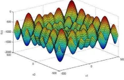
4.1. Schwefel Function
The Schwefel function (Figure 1) is given by the following analytical expression:
1
1
( )
418.9829 *
sin
D
i i
i
f x
D
x
x
(4.1)The search space for this function is restricted to -500 ≤xi ≤ 500, i =1, …, D, D is the number
of dimensions. The maximum value of this test problem for two dimensions is fopt = 0.
4.2. Schwefel Problem 1.2
This test function (Figure 2) is given as:
2
2
1 1
( )
D i
j i j
f x x
(4.2)The test problem has the following search range: -100 ≤ xj ≤ 100. In this equation D is the
number of dimensions.
This function is explored for two dimensions and its maximum is fopt = 0.
4.3. Schwefel Problem 2.22
The Schwefel Problem 2.22 (Figure 3) is a global optimization function with the following definition:
3
1 1
( )
D D
i i
i i
f x
x
x
(4.3)where search space borders are defined by -10 ≤xi ≤ 10, I = 1, …, D and D is the number of
dimensions. The maximum value of this test problem for two dimensions is fopt = 0.
4.4. Branin Function
The Branin function (Figure 4.) is a two-dimensional optimization function which is defined as:
2 2
4 2 2 1 1 1
5.1
5
1
( )
6
10 1
cos
10
4
8
f x
x
x
x
x
(4.4)The search domain of this test problem for x1 is [-5;10] and for x2 is [0;15]. The maximum
value is fopt = -0.398.
Figure 3: Schwefel Problem 2.22 2D Figure 4: Branin function 2D
5. Experimental Results
Two sets of experiments of 320 evaluations per function are made for 100 and 2000 generations. The results are accepted as successful if: for Schwefel function they are higher than -0.5; for Schwefel Problem 1.2 they are higher than -0.5; for Schwefel Problem 2.22 they are higher than -0.3; for Branin function they are higher than -0.4. All results are showed in the following table:
Table 1: Experimental results
f
Number of the
successful results Results (%)
100G 2000G 100G 2000G
1
f 260 298 81.25% 93.13%
2
f 305 316 95.31% 98.75%
3
f 319 320 99.69% 100%
4
6. Conclusion
In this study different test functions are explored, because they are resistant to traditional approximation techniques.
For this purpose whole test problems are developed with the same black-box model of the algorithm. When using this model to solve the function is not necessary to reset the algorithm itself and is not necessary to change the parameters of this algorithm.
Two different series were made for each test function for 100 generations and for 2000 generations. The experimental results show that the average success of the algorithm for 100 generations is 92.95% and for 2000 generations is 97.97%.
Schwefel function, Schwefel Problem 1.2 and Schwefel Problem 2.22 which are tested for two dimensions in this exploration, can be tasted for more dimensions. Furthermore other functions can be tested with DE algorithm.
References
1. Dantzig G. B., "The Nature of Mathematical Programming, "Mathematical Programming
Glossary", INFORMS Computing Society.
2. J. Ilonen, J.-K. Kamarainen, and J. Lampinen, “Differential evolution training algorithm for feed-forward neural networks”, Neural Process.Lett., Vol. 7, No. 1, pp. 93-105, 2003.
3. Penev K., 2005. Adaptive search heuristics applied to numerical optimisation, pp.47-51, PhD thesis, SSU.
4. Penev, K., 2006. Free Search and Differential Evolution Towards Dimensions Number Change. In: Intelligent Engineering Systems Through Artificial Neural Networks. ASME, New York, USA, pp. 37-42. ISBN 0-7918-0256-6
5. Price K., and Srorn R., 1997, Differential Evolution – A simple evolution strategy for fast optimisation, Dr. Dobb’s Journal, Vol. 22 (4), pp. 18-24.
6. Qin A., Huang V., Suganthan, 2008, Differential Evolution Algorithm With Strategy Adaptation for Global Numerical Optimization
7. Joshi R. and Sanderson A. C., “Minimal representation multisensory fusion using differential evolution”, IEEE Trans. Syst. Man. Cybern A, Syst. Humans, Vol. 29, No. 1, pp. 63-76, Jan. 1999.
8. Storn R., ”On the usage of differential evolution for function optimization”, Proc. Biennial Conf. North Amer. FuzzyInf. Process. Soc., Berkeley, CA, 1996, pp. 519-523.