The Thirty-Third AAAI Conference on Artificial Intelligence (AAAI-19)
Multiple Independent Subspace Clusterings
Xing Wang,
1Jun Wang,
1∗Carlotta Domeniconi,
2Guoxian Yu,
1,3Guoqiang Xiao,
1Maozu Guo
41College of Computer and Information Sciences, Southwest University, Chongqing, China 2Department of Computer Science, George Mason University, Fairfax, USA
3Hubei Key Laboratory of Intelligent Geo-Information Processing, China University of Geosciences, Hubei, China 4School of Electrical and Information Engineering, Beijing University Of Civil Engineering and Architecture, Beijing, China
Email:{wx1993cs,kingjun,gxyu,gqxiao}@swu.edu.cn, [email protected], [email protected]
Abstract
Multiple clustering aims at discovering diverse ways of orga-nizing data into clusters. Despite the progress made, it’s still a challenge for users to analyze and understand the distinc-tive structure of each output clustering. To ease this process, we consider diverse clusterings embedded in different sub-spaces, and analyze the embedding subspaces to shed light into the structure of each clustering. To this end, we provide a two-stage approach called MISC (Multiple Independent Sub-space Clusterings). In the first stage, MISC uses independent subspace analysis to seek multiple and statistical independent (i.e. non-redundant) subspaces, and determines the number of subspaces via the minimum description length principle. In the second stage, to account for the intrinsic geometric structure of samples embedded in each subspace, MISC per-forms graph regularized semi-nonnegative matrix factoriza-tion to explore clusters. It addifactoriza-tionally integrates the kernel trick into matrix factorization to handle non-linearly separa-ble clusters. Experimental results on synthetic datasets show that MISC can find different interesting clusterings from the sought independent subspaces, and it also outperforms other related and competitive approaches on real-world datasets.
Introduction
Clustering is an unsupervised learning technique that aims at partitioning data into a number of homologous groups (or clusters). However, traditional clustering methods typically provide a single clustering, and fail to reveal the diverse pat-terns underlying the data. In fact, several different clustering solutions may co-exist in a given problem, and each may provide a reasonable organization of the data, e.g., people can be assigned to different communities based on different roles; proteins can be categorized differently based on their amino acid sequences or their 3D structure. In these sce-narios, it would be desirable to present multiple alternative clusterings to the users, as these alternative clusterings can explain the underlying structure of the data from different viewpoints.
To address the aforementioned problem, the research field of multi-clustering has emerged during the last decade. Naive solutions run a single clustering algorithm with
dif-∗
Corresponding author, [email protected] (Jun Wang) Copyright c2019, Association for the Advancement of Artificial Intelligence (www.aaai.org). All rights reserved.
ferent parameter values, or explore different clustering al-gorithms (Bailey 2013). These approaches may generate multiple clusterings with high redundancy, since they do not take into account the already explored clusterings. To overcome this drawback, two general strategies have been introduced. The first one simultaneously generates multi-ple clusterings, which are required to be different from each other (Jain, Meka, and Dhillon 2008; Dang and Bailey 2010). The second one generates multiple clusterings in a greedy manner, and forces the new clusterings to be different from the already generated ones (Cui, Fern, and Dy 2007; Hu et al. 2015; Yang and Zhang 2017).
Most of these clustering methods consider multi-ple clusterings in the full feature space. However, as the di-mensionality of the data increases, clustering methods en-counter the challenge of the curse of dimensionality (Par-sons, Haque, and Liu 2004). Furthermore, some features may be relevant to some clusterings but not others. This phe-nomenon is also observed in data with moderate dimension-ality. Subspace clustering aims at finding clusters in sub-spaces of the original feature space, but it faces an expo-nential (2d−1) search space and focuses on exploring only
one clustering. Some approaches try to find alternative clus-terings in a weighted feature space (Caruana et al. 2006; Hu et al. 2015) or in a transformed feature space (Cui, Fern, and Dy 2007; Davidson and Qi 2008); however, the former methods cannot control well the redundancy between differ-ent clusterings, and the latter cannot find multiple orthogonal subspaces at the same time.
To overcome these issues, we propose an approach called Multiple Independent Subspace Clusterings (MISC) to ex-plore diverse clusterings in multiple independent subspaces, one clustering for each subspace. During the first stage, MISC uses Independent Subspace Analysis (ISA) (Szab´o, P´oczos, and L˝orincz 2012) to explore multiple pairwise-independent (i.e., non-redundant) subspaces by minimizing the mutual information among them, and seeks the num-ber of independent subspaces via the minimum description length principle (Rissanen 2007). MISC automatically deter-mines the number of clusters in each subspace via Bayesian
data into a reproducing kernel Hilbert space via the kernel trick.
This paper makes the following contributions:
• We introduce an approach called MISC to explore multi-ple clusterings in independent subspaces. MISC automat-ically computes the number of independent subspaces, which provide multiple individual views of the data.
• MISC leverages graph regularized semi-nonnegative ma-trix factorization and kernel mapping to group non-linearly separable clusters, and can determine the number of clusters in each subspace.
• Experimental results show that MISC can explore differ-ent clusterings in various subspaces, and it significantly outperforms other related and competitive approaches (Caruana et al. 2006; Bae and Bailey 2006; Cui, Fern, and Dy 2007; Davidson and Qi 2008; Jain, Meka, and Dhillon 2008; Hu et al. 2015; Yang and Zhang 2017; Niu, Dy, and Jordan 2010; Guan et al. 2010; Niu, Dy, and Ghahramani 2012).
Related Work
Existing multi-clustering approaches can be classified into two categories depending on how they control redundancy, either based on clustering labels, or on feature space.
COALA (Constrained Orthogonal Average Link Algo-rithm) (Bae and Bailey 2006) is the classic algorithm that controls redundancy through clustering labels. It transforms linked pairs of the reference clustering into cannot-link con-straints, and then uses agglomerative clustering to find an alternative clustering. MNMF (Multiple clustering by Non-negative Matrix Factorization) (Yang and Zhang 2017) de-rives a diversity regularization term from the labels of exist-ing clusterexist-ings, and then integrates this term with the ob-jective function of NMF to seek another clustering. The performance of both COALA and MNMF heavily depends on the quality of already discovered clusterings. To alle-viate this issue, other methods simultaneously seek multi-ple clusterings by minimizing the correlation between the labels of two distinct clusterings and by optimizing the quality of each clustering (Jain, Meka, and Dhillon 2008; Wang et al. 2018). For example, De-kmeans (Decorrelated
k-means) (Jain, Meka, and Dhillon 2008) simultaneously learns two disparate clusterings by minimizing ak-means sum squared error objective for the two clustering solutions, and by minimizing the correlation between the two cluster-ings. CAMI (Clustering for Alternatives with Mutual Infor-mation) (Dang and Bailey 2010) optimizes a dual-objective function, in which the log-likelihood objective (accounting for the quality) is maximized, while the mutual information objective (accounting for the dissimilarity) of pairwise clus-terings is minimized.
Multi-clustering solutions that explore multiple cluster-ings using a feature-based criterion have also been stud-ied. Some of them assign weights to features. For example, MetaC (Meta Clustering) (Caruana et al. 2006) first applies
k-means to generate a large number of base clusterings us-ing weighted features based on the Zipf distribution (Zipf
1949), and then obtains multiple clusterings via a hierarchi-cal clustering ensemble. MSC (Multiple Stable Clusterings) (Hu et al. 2015) detects multiple stable clusterings in each weighted feature space using the idea of clustering stabil-ity based on Laplacian Eigengap. Unfortunately, MSC can-not guarantee diversity among multiple clusterings, since it cannot control the redundancy very well. Other feature-wise multi-clusterings are based on transformed features. They use a data space S to characterize the existing clusterings and try to construct a new feature space, which is either or-thogonal toS, or independent fromS. Once the novel fea-ture space is constructed, any clustering algorithm can be used in this space to generate an alternative clustering. OSC (Orthogonal subspace clustering) (Cui, Fern, and Dy 2007) transforms the original feature space into an orthogonal sub-space using a projection framework based on the given clus-tering, and then groups the transformed data into different clusters. ADFT (Alternative Distance Function Transforma-tion) (Davidson and Qi 2008) adopts a distance metric learn-ing technique (Xlearn-ing et al. 2003) and slearn-ingular value decom-position to obtain an alternative orthogonal subspace based on a given clustering. Thereafter, it obtains an alternative clustering by running the clustering algorithm in the new orthogonal feature space. mSC (Multiple Spectral Cluster-ings) (Niu, Dy, and Jordan 2010) finds multiple clusterings by augmenting a spectral clustering objective function, and by using the Hilbert-Schmidt independence criterion (HSIC) (Gretton et al. 2005) among multiple views to control the re-dundancy. NBMC (Nonparametric Bayesian Multiple Clus-tering) (Guan et al. 2010) and NBMC-OFV (Nonparametric Bayesian model for Multiple Clustering with Overlapping Feature Views) (Niu, Dy, and Ghahramani 2012) both em-ploy a Bayesian model to explore multiple feature views and clusterings therein.
Feature-based multiple clustering methods typically seek a full space transformation matrix, or measure the similar-ity between samples in the full space. Therefore, their per-formance may be compromised with high-dimensional data. Furthermore, some data only show cluster structure on a sub-set of features. Given the above analysis, we advocate to separately explore diverse clusterings in independent sub-spaces, and introduce an approach called MISC. MISC first uses independent subspace analysis to obtain multiple in-dependent subspaces, and then performs clustering in each independent subspace to achieve multiple clusterings. Ex-tensive experimental results show that MISC can effectively uncover multiple diverse clusterings in each identified sub-space.
Proposed Approach
MISC consists of two phases: (1) Finding multiple indepen-dence subspaces, and (2) Exploring a clustering in each sub-space. In the following, we provide the details of each phase.
Independent Subspace Analysis
Hoyer, and Inki 2001). Let’s consider a data matrix X ∈
Rd×n fornsamples withdfeatures. ICA describesXas a
linear mixture of sources, i.e., AS = X ∈ Rd×n, where
A ∈ Rd×d is the mixing matrix andScorresponds to the
source components. The source matrix S ∈ Rd×n
repre-sentsn observations under multiple independent row vec-tors, i.e.,S= (S1;S2;· · ·;Sd), where eachSicorresponds
to a source component.
Unlike ICA, which requires pairwise independence be-tween all individual source components, Independence Sub-space Analysis (ISA) aims at finding a linear transforma-tion of the given data, and it yields several jointly indepen-dent source subspaces, each of which contains one or more source components. Let’s assume there arev independent subspaces; ISA seeks the corresponding source subspaces
S(1),· · · ,S(v) by minimizing the mutual information be-tween pairwise subspaces as follows:
minMI(S(1),· · ·,S(v)) (1)
Various ISA solvers are available, and they vary in terms of the applied cost functions and optimization tech-niques (Szab´o, P´oczos, and L˝orincz 2012). For example, fastISA(Hyv¨arinen and K¨oster 2006) seeks the mixing ma-trixAby iteratively updating its rows in a fixed-point man-ner. Unfortunately, fastISA can only find equal-sized sub-spaces, while multiple clusterings may exist in subspaces of different sizes. Here we adopt a variant of ISA (Szab´o, P´oczos, and L˝orincz 2012), which makes use of the “ISA separation principle”, stating that ISA can be solved by first performing ICA, and then searching and merging the com-ponents. As such, the independence between the groups is maximized, and the groups do not need to have an equal number of components. This ISA solution only needs to specify the number of subspacesv, which is difficult to de-termine. To compute the number of subspaces, we use a greedy search strategy, which combines agglomerative clus-tering and Minimum Description Length (MDL) principle (Rissanen 2007).
The first step of agglomerative clustering is to merge sub-spaces. Given two subspacesS(i)andS(j), we compute their
independence as follows:
CI(S(i),S(j)) =CH(S(i)∪S(j))−CH(S(i))−CH(S(j))
(2) whereCH(S) = |S2| ·log2(n) +
Pn i=1log2
1
fS(S·i) is the
entropy cost to encode thenobjects in the subspaceSusing the probability-density function f1
S, which can be obtained using kernel density estimation1. We computeC
I of each
pair of subspaces and merge the subspaces with the smallest
CI. We repeat the above step until the number of subspaces
v <2, or all theCI >0.
We apply the MDL principle to determine the number of subspaces. MDL is widely used for model selection. Its core idea is to choose the model, which allows a receiver to exactly reconstruct the original data using the most suc-cinct transmission. MDL balances the coding length of the model and the coding length of the deviations of the data
1
https://bitbucket.org/szzoli/ite/downloads/
from that model. More concretely, the coding cost for trans-mitting dataDtogether with a modelM is
L(D, M) =L(M) +L(D|M) (3)
When subspaces are merged in each iteration, we update
L(D, M). Finally, we choose the number of subspacesv
corresponding to the smallestL(D, M). Concretely, we use the technique in (Rissanen 2007; Ye et al. 2016) to measure the length of the model and data coding as follows:
L(M) = d
2
2 ·log2(n) + (v+ 1)·log2(d) (4)
L(D|M) = d
2 ·log2(n) +
v X
i=1
n X
j
log2
1
fS(S
(i)
·j )
(5)
wherenis the number of samples,dis the number of fea-tures, and fS(S
(i)
·j ) is the probability-density function for
each subspace. As a result, we obtain v independent sub-spaces.
Exploring Multiple Clusterings
After obtaining multiple independent subspaces, we use Bayesian k-means (Welling 2006) to guide the computa-tion of the number of clusters in each subspace. Bayesian
k-means adopts a variational Bayesian framework (Ghahra-mani and Beal 1999) to iteratively choose the optimal num-ber of clusters. We then perform Graph regularized Semi-NMF (GSSemi-NMF) to cluster data embedded in each subspace. GSNMF is an improvement upon SNMF by leveraging the geometric structure of samples to regularize the matrix fac-torization.
SNMF (Ding, Li, and Jordan 2010) is a variant of the clas-sical NMF (Lee and Seung 1999); it extends the application of traditional NMF from nonnegative inputs to mix-signed inputs. At the same time, it preserves the strong clustering interpretability. The objective function of SNMF can be for-mulated as follows:
JSN M F =kX−ZHk2s.t.H≥0 (6)
whereZ∈Rd×kcan be viewed as the cluster centroids, and H ∈Rk×n,H ≥0is the soft cluster assignment matrix in
the latent space. We can transform the soft clusters to hard clusters by clustering the index matrixH.
Inspired by GNMF (Graph regularized Nonnegative Ma-trix Factorization) (Cai et al. 2011), we make use of the in-trinsic geometric structure of samples to guide the factoriza-tion ofH, and cascade it toZ. As a result, we obtain the fol-lowing objective function for the graph regularized SNMF (GSNMF):
JGSN M F =kX−ZHk2+λtr(HLHT) (7)
wheretr(·)denotes the trace of a matrix,λ≥0is the regu-larization parameter;L∈Rn×nis the graph Laplacian
ma-trix L = D−P, P ∈ Rn×n is the weighted adjacency
matrix of the graph (Cai et al. 2011),D∈Rn×nis the
minimizing the graph regularized term, we assume that if
X·jandX·iare close to each other, then their cluster labels H·iandH·jshould be close as well.
However, GSNMF, similarly to NMF and SNMF, does not perform well with data that are non-linearly separable in in-put space. To avoid this potential issue, we consider map-ping the data points onto a Reproducing kernel Hilbert space
φ(X), and reformulate Eq. (7) as follows:
JKGSN M F =kφ(X)−ZHk2+λT r(HLHT) (8)
This formulation makes it difficult to computeZandH, since they depend on the mapping functionφ(·). To solve this problem, we add constraints on the basis vectorsZ. As such, the basis matrix Zcan be further formulated as the combination of weighted-samplesZ = φ(X)W, in which
W ≥ 0 is the weight matrix. Eq. (8) can be rewritten as follows:
JKGSN M F =kφ(X)−φ(X)WHk2+λT r(HLHT)
s.t.W≥0;H≥0
(9) Through kernel mapping, KGSNMF can properly cluster, not only linearly separable data, but also non-linearly sep-arable ones.
Optimization: We follow the idea of standard NMF to optimize W and H by an alternating optimization tech-nique. Particularly, we alternate the optimization ofWand
H, while fixing the other as constant. For simplicity, we use
φto representφ(X).
OptimizingJKGSN M F with respect toWis equivalent
to optimizing the following function:
J1(W) =kφ−φWHk2 (10)
To embed the constraintW≥0, we introduce the Lagrange multiplierΦ∈Rn×k:
L(W) =kφ−φWHk2−ΦWT (11)
Letting the partial derivative ∂L∂(WW)= 0, we obtain
Φ= (φTφ+φTφWH)HT (12)
Based on the Karush-Kuhn-Tucker (KKT) (Boyd and Van-denberghe 2004) complementarity conditionΦijWij = 0,
we have:
[(φTφ+φTφWH)HT]ijWij= 0 (13)
Eq. (13) leads to the following updating formula forW:
Wij←Wij s
[φTφ]+HT + [φTφ]−WHHT ij
[φTφ]−HT + [φTφ]+WHHT ij
(14)
where we separate the positive and negative parts ofφTφby
setting[φTφ]+ = (|φTφ|+φTφ)/2,[φTφ]− = (|φTφ| −
φTφ)/2.
Similarly, we can get the updating formula forH:
Hij ←Hij v u u t
WT[φTφ]++WT[φTφ]+WH+λ[HL]−
ij
WT[φTφ]++WT[φTφ]+WH+λ[HL]+
ij
(15)
From Eq. (14) and Eq. (15), we can see that the updating for-mulas do not depend on the mapping functionφ(·), and we can computeφ(X·i)Tφ(X·j) via any kernel function, i.e.,
φ(X·i)Tφ(X·j) =κ(X·i,X·j).
By iteratively applying Eqs. (14) and (15) in each inde-pendent subspace, we can obtain the optimizedW∗andH∗. EachH∗ obtained from each subspace corresponds to one clustering. As such, we obtainvclusterings fromv indepen-dent subspaces.
Algorithm 1 presents the whole MISC procedure. Line 1 computes the source matrix Svia independent component analysis; Line 2 merges the subspaces according to Eq.(2) and using agglomerative clustering, and saves the MDL (Lmin) for each merge; Line 3 chooses the best set of
sub-spacesΩminwith the minimum MDL (Li) through a sorting
operation; Lines 5-9 cluster data for each subspace though KGSNMF; Lines 10-18 give the procedure of KGSNMF.
Algorithm 1MISC: Multiple Independent Subspace Clus-terings
Input: X: dataset ofnsamples withdfeatures; Output: {Ci}v
i=1:vclusterings.
1: S=ICA(X)
2: {Li,Ωi}di=1= MergeSubspace(S) /*agglomerative
clus-teringS;Ωi is the set of subspaces afteri-th mergeing
andLiis the MDL corresponding toΩi*/ 3: {Lmin,Ωmin}=sort({Li,Ωi}).
/*Ωmin={S(1),S(2),· · ·,S(v)}*/ 4: Forj= 1 :|Ωmin|
5: kj= Bayesiank-means(S(j)) 6: H(j)= KGSNMF(S(j), k
j) 7: Cj=k-means(H(j), kj) 8: End For
9: FunctionH= KGSNMF(X,k)
10: InitializeWandHrandomly.
11: /* Compute kernel similar matrix*/
12: [φ(X·i)Tφ(X·j)] =κ(X·i,X·j) 13: Whilenot convergedDo
14: UpdateWusing Eq. (14);
15: UpdateHusing Eq. (15);
16: End While
17: End Function
Complexity analysis
The complexity of ISA is O(d2n)and the complexity of
MDL isO(dn2)(for each merge). Since we need to merge the subspaces for at mostdtimes, the overall time complex-ity of the first stage is O(d(d2n+dn2)). For the second
stage, MISC takes O(n2d)time to construct the p-nearest
neighbor graph. Assuming the multiplicative updates stop after t iterations and the number of clusters isk, then the cost for KGSNMF isO(tdkn+n2d). In summary, the
Experiments
Experiments on synthetic data
We first conduct two types of experiments on synthetic data, the first type of experiments is to prove that MISC can find multiple independent subspaces, and the second type is to prove that our KGSNMT has a better clustering performance than SNMF.
The first synthetic data contains four subspaces consist-ing of800samples with8features: the first subspace con-tains four clusters, corresponding to the shapes of the digits ‘2’,‘0’,‘1’,‘9’ (Fig. 1(a)); the second subspace also contains four clusters, corresponding to the shapes of the letters ‘A’ (three shapes) and‘I’ (Fig. 1(b)); the third one contains six clusters generated by a Gaussian distribution (Fig. 1(c)); the last one contains two clusters, which are non-linearly sepa-rable (Fig. 1(d)). To ensure the non-redundancy among the four subspaces, we randomly permute the sample index in each subspace before merging them into a full space. Note that the synthetic data is diverse; it includes subspaces with the same scale, such as the first and the second subspaces, as well as subspaces with different scales, such as the second, third, and fourth subspaces. We choose the Gaussian heat kernel as the kernel function and the kernel width is set to the standard varianceσ =sqrt(Pni=1 k X·i−X k2 /n).
Following the set of GNMF in (Cai et al. 2011), we use 0-1 weighting and adopt the neighborhood size = 5 to com-pute the graph adjacency matrixP, and then setλ= 10in Eq. (8). We apply MISC on the first synthetic dataset and plot the found subspace views and clustering results in the last four subfigures of Fig. 1.
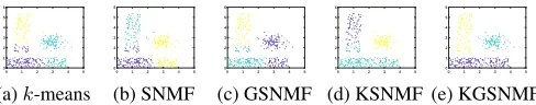
The first view shown in Fig. 1(e) corresponds to the sec-ond original subspace; the secsec-ond view shown in Fig. 1(f) corresponds to the first original subspace; the third view shown in Fig. 1(g) corresponds to the third original sub-space; and the fourth view shown in Fig. 1(h) corresponds to the fourth original subspace. Due to the ISA procedure, the original feature space has been normalized and converted into the new space, so the four original subspaces are similar to the four subspaces found by MISC, but not identical. The relative position of each cluster in the new subspace is still the same as before, but the new subspaces are rotated and stretched because ICA tries to find subspaces which are lin-ear combinations of the original ones. For each subspace, we use KGSNMF to cluster the data. KGSNMF correctly iden-tifies the clusters for the first, third, and fourth views; the second one is approximately close to the original one. Since KGSNMF accounts for the intrinsic geometric structure and for non-linearly separable clusters, it obtain good clustering results on both non-linearly separable and spherical clusters. The second and third synthetic datasets are collected from the Fundamental Clustering Problem Suite (FCPS)2. We use them to investigate whether KGSNMF achieves a better clustering performance than SNMF. Atom, the second syn-thetic dataset, consists of800 samples with three features. It contains two nonlinearly separable clusters with differ-ent variance as shown in Fig. 2. Lsun, the third synthetic
2
http://www.uni-marburg.de/fb12/datenbionik/downloads/FCPS
dataset, consists of 400samples with two features. It con-tains three clusters with different variance and inner-cluster distance as shown in Fig. 3. We choose a Gaussian kernel and setλ= 10 for KGSNMF and GSNMF as before. The clustering results on Atom are plotted in Fig. 2, and we can see that both KSNMF and KGSNMF correctly separate the two clusters, whilek-means, SNMF, and GSNMF do not. This is because the introduced kernel function could map the nonlinearly separable space to a high-dimensional lin-early separable space. The clustering results for Lsun are shown in Fig. 3.k-means, SNMF, GSNMF, and KSNMF do not cluster the data very well.k-means, SNMF, and GSNMF are all influenced by the distribution of the clusters at the bottom. KSNMF can mitigate the impact, but it still cannot perfectly separate the clusters, whereas KGSNMF can do the job correctly. Overall, KSNMF achieves good clustering re-sults especially on nonlinearly separable clusters, such as on Atom. The impact of different structures could be alleviated to some extent on both linearly and nonlinearly separable data. The embedded graph regularized term can better repre-sent the details of the intrinsic geometry of the data; as such KGSNMF obtains better clustering results than KSNMF.
0 5 10 15 20
feature 1 0 5 10 15 20 feature 2 (a) Subspace1
0 5 10 15 20
feature 3 0 5 10 15 20 feature 4 (b) Subspace2
30 40 50 60 70 80
feature 5 20 40 60 80 100 120 feature 6 (c) Subspace3
-40 -20 0 20 40
feature 7 -40 -20 0 20 40 feature8 (d) Subspace4
-2 -1 0 1 2
feature 1 -2 -1 0 1 2 feature 2 (e) View1
-2 -1 0 1 2
feature 3 -2 -1 0 1 2 feature 4 (f) View2
-2 -1 0 1 2
feature 5 -2 -1 0 1 2 feature 6 (g) View3
-3 -2 -1 0 1 2 3
feature 7 -3 -2 -1 0 1 2 3 feature 8 (h) View4
Figure 1: Four different clusterings in four subspaces (a-d), and the four clusterings explored by MISC (e-h).
-50 50 50 0 0 50 0 -50-50
(a)k-means
-50 50 50 0 0 50 0 -50-50 (b) SNMF -50 50 50 0 0 50 0 -50-50 (c) GSNMF -50 50 50 0 0 50 0 -50-50 (d) KSNMF -50 50 50 0 0 50 0 -50-50 (e) KGSNMF
Figure 2: Results of different clustering algorithms on the synthetic dataset Atom.
0 1 2 3 4 5 0 1 2 3 4 5 6
(a)k-means
0 1 2 3 4 5 0 1 2 3 4 5 6 (b) SNMF
0 1 2 3 4 5 0 1 2 3 4 5 6 (c) GSNMF
0 1 2 3 4 5 0 1 2 3 4 5 6 (d) KSNMF
0 1 2 3 4 5 0 1 2 3 4 5 6 (e) KGSNMF
Experiments on real-world datasets
We test MISC on four real-world datasets wildly used for multiple clustering, including a color image dataset, two gray image datasets, and a text dataset.
• Amsterdam Library of Object Images dataset. The ALOI dataset3 consists of images of 1000 common
ob-jects taken from different angles and under various illu-mination conditions. We have chosen four objects: green box, red box, tennis ball, and red ball, with different col-ors and shapes from different viewing directions for a to-tal of 288 images (Fig. 4). Following the preprocessing in (Dalal and Triggs 2005), we extracted 840 features4and further applied Principle Component Analysis (PCA) to reduce the number of features to 49, which retain more than 90% variance of the original data.
• Dancing Stick Figures dataset. The DSF dataset (G¨unnemann et al. 2014) consists of 900 samples of 20×20images with random noise across nine stick fig-ures. (Fig. 5). The nine raw stick figures are obtained by arranging in three different positions the upper and lower body; this provides two views for the dataset. As for the ALOI, we also applied PCA, and retained more than 90% of the data’s variance as preprocessing.
• CMUface dataset.The CMUface dataset5 contains 640 grey32×20images of 20 individuals with varying poses (up, straight, right, and left). As such, it can be clustered either by identity or by pose. Again, we apply PCA to reduce the dimensionality while retaining more than 90% of the data’s variance.
• WebKB datasetThe WebKB dataset6contains html
doc-uments from four universities: Cornell University; Uni-versity of Texas, Austin; UniUni-versity of Washington; and University of Wisconsin, Madison. The pages are addi-tionally labeled as being from 4 categories: course, fac-ulty, project, and student. We preprocessed the data by removing rare words, stop words, and words with a small variance, retaining 1041 samples and 456 words.
Figure 4: Four objects of different shapes (box and ball) and colors (green and red) from ALOI.
Figure 5: Nine raw samples of the Dancing Stick Figures.
We compare MISC with MetaC, MSC, OSC, COALA, De-kmeans, ADFT, MNMF, mSC, NBMC, and NBMC-OFV (all methods are discussed in the related work section).
3
http://aloi.science.uva.nl/
4https://github.com/adikhosla/feature-extraction
5
http://archive.ics.uci.edu/ml/datasets.html 6
http://www.cs.cmu.edu/ webkb/
The input parameters of these algorithms were set or opti-mized as suggested by the authors. We also set the number of subspaces as 2 and the number of clusters as that of true labels of CMUface and WebKB datasets, respectively.
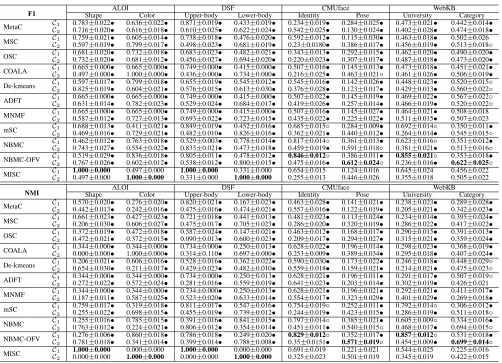
We visualize the clustering results of MISC for the first three image datasets in Figs. 6-8, and use the widely-known F1-measure (F1) and normalized mutual information (NMI) to evaluate the quality of the clusterings. Since we don’t know which view the clustering corresponds to, we com-pare each clustering with the true label under each view, and finally compute the confusion matrix and report the results (average of ten independent repetitions) in Table 1.
cluster 1 cluster 2
(a) Subspace1: shape
cluster 1 cluster 2
(b) Subspace2: color
Figure 6: ALOI dataset: Mean images of the clusters in two subspaces detected by MISC from the perspective of shape (a) and color (b).
cluster 1 cluster 2 cluster 3
(a) Subspace1: upper-body
cluster 1 cluster 2 cluster 3
(b) Subspace2: lower-body
Figure 7: DSF dataset: Mean images of the clusters in two subspaces detected by MISC from the perspective of the upper-body (a) and lower-body (b).
(a) Subspace1: identity (b) Subspace2: pose
Figure 8: The mean image of the clusters of two clusterings in two subspaces of CMUface detected by MISC from the perspective of identity (a) and pose (b).
Table 1: F1 and NMI confusion matrix (Mean±Std).C1andC2indicate two clusterings of the same data.•/◦indicates whether
MISC is statistically (according to pairwiset-test at 95% significance level) superior/inferior to the other method. The bold numbers represent the best results.
F1 Shape ALOI Color Upper-body DSFLower-body IdentityCMUface Pose UniversityWebKB Category
MetaC CC1 0.783±0.022• 0.636±0.022• 0.871±0.019• 0.433±0.019• 0.234±0.019• 0.284±0.025• 0.473±0.021• 0.442±0.014•
2 0.716±0.020• 0.616±0.018• 0.610±0.025• 0.622±0.024• 0.542±0.025• 0.130±0.024• 0.402±0.028• 0.474±0.018•
MSC CC1 0.759±0.021• 0.605±0.014• 0.738±0.018• 0.476±0.020• 0.592±0.012• 0.115±0.030• 0.463±0.018• 0.502±0.026
2 0.597±0.019• 0.799±0.017• 0.498±0.023• 0.681±0.019• 0.23±0.0180• 0.386±0.017• 0.456±0.019• 0.513±0.018◦
OSC CC1 0.681±0.020• 0.732±0.018• 0.683±0.023• 0.482±0.021• 0.343±0.013• 0.292±0.015• 0.462±0.020• 0.490±0.020•
2 0.732±0.020• 0.681±0.012• 0.456±0.027• 0.694±0.020• 0.220±0.023• 0.307±0.017• 0.487±0.018• 0.473±0.020•
COALA CC1 0.665±0.000• 0.665±0.000• 0.749±0.000• 0.415±0.000• 0.507±0.016• 0.145±0.013• 0.473±0.018• 0.451±0.021•
2 0.497±0.000• 1.000±0.000• 0.436±0.000• 0.734±0.000• 0.216±0.025• 0.463±0.021◦ 0.461±0.026• 0.506±0.019•
De-kmeans CC1 0.597±0.017• 0.799±0.018• 0.655±0.019• 0.545±0.012• 0.545±0.016• 0.142±0.026• 0.448±0.023• 0.520±0.015◦
2 0.825±0.019• 0.604±0.021• 0.576±0.015• 0.613±0.030• 0.376±0.028• 0.123±0.017• 0.429±0.013• 0.560±0.022◦
ADFT CC1 0.665±0.000• 0.665±0.000• 0.749±0.000• 0.415±0.000• 0.507±0.022• 0.145±0.019• 0.469±0.022• 0.567±0.022◦
2 0.631±0.014• 0.782±0.023• 0.529±0.024• 0.684±0.017• 0.419±0.026• 0.257±0.014• 0.466±0.019• 0.520±0.022◦
MNMF C1 0.665±0.000• 0.665±0.000• 0.749±0.000• 0.415±0.000• 0.507±0.016• 0.145±0.027• 0.464±0.021• 0.508±0.018
C2 0.587±0.012• 0.727±0.013• 0.693±0.022• 0.723±0.015• 0.435±0.022• 0.225±0.022• 0.511±0.015• 0.507±0.023
mSC C1 0.688±0.013• 0.411±0.021• 0.849±0.019• 0.452±0.016• 0.685±0.015◦ 0.284±0.009• 0.692±0.014◦ 0.350±0.011•
C2 0.469±0.016• 0.729±0.021• 0.482±0.010• 0.826±0.016• 0.362±0.021• 0.440±0.012• 0.264±0.014• 0.545±0.015◦
NBMC CC1 0.462±0.012• 0.763±0.018• 0.529±0.003• 0.778±0.014• 0.817±0.014◦ 0.361±0.013• 0.623±0.016◦ 0.351±0.012•
2 0.743±0.027• 0.554±0.022• 0.833±0.021• 0.473±0.018• 0.459±0.019• 0.591±0.018◦ 0.381±0.021• 0.513±0.016◦
NBMC-OFV CC1 0.519±0.029• 0.836±0.018• 0.805±0.011• 0.478±0.012• 0.846±0.012◦ 0.386±0.011• 0.855±0.021◦ 0.353±0.018•
2 0.767±0.026• 0.602±0.012• 0.538±0.012• 0.800±0.015• 0.475±0.016• 0.612±0.024◦ 0.236±0.016• 0.622±0.025◦
MISC CC1 1.000±0.000 0.497±0.000 1.000±0.000 0.331±0.000 0.654±0.015 0.124±0.016 0.645±0.024 0.456±0.022
2 0.497±0.000 1.000±0.000 0.331±0.000 1.000±0.000 0.255±0.013 0.446±0.026 0.355±0.018 0.505±0.022
NMI Shape ALOI Color Upper-body DSFLower-body IdentityCMUface Pose UniversityWebKB Category
MetaC CC1 0.570±0.020• 0.276±0.020• 0.820±0.021• 0.167±0.023• 0.463±0.028• 0.141±0.021• 0.238±0.023• 0.289±0.028•
2 0.442±0.013• 0.242±0.016• 0.475±0.016• 0.474±0.021• 0.557±0.016• 0.122±0.019• 0.205±0.021• 0.342±0.023•
MSC CC1 0.661±0.023• 0.427±0.023• 0.721±0.018• 0.441±0.013• 0.481±0.023• 0.113±0.024• 0.234±0.014• 0.395±0.024•
2 0.206±0.030• 0.606±0.027• 0.475±0.017• 0.705±0.023• 0.286±0.020• 0.320±0.019• 0.286±0.022• 0.417±0.022•
OSC CC1 0.372±0.019• 0.472±0.018• 0.587±0.024• 0.147±0.021• 0.463±0.012• 0.168±0.017• 0.290±0.015• 0.391±0.013•
2 0.472±0.021• 0.372±0.015• 0.090±0.013• 0.600±0.023• 0.209±0.017• 0.294±0.027• 0.315±0.021• 0.359±0.024•
COALA CC1 0.344±0.000• 0.344±0.000• 0.734±0.000• 0.250±0.013• 0.628±0.022• 0.196±0.014• 0.298±0.023• 0.368±0.019•
2 0.000±0.000• 1.000±0.000• 0.314±0.110• 0.697±0.000• 0.253±0.009• 0.389±0.034• 0.295±0.018• 0.407±0.024•
De-kmeans CC1 0.206±0.021• 0.606±0.016• 0.528±0.016• 0.362±0.022• 0.590±0.030• 0.173±0.022• 0.246±0.018• 0.448±0.029◦
2 0.654±0.030• 0.211±0.017• 0.429±0.023• 0.482±0.010• 0.559±0.018• 0.159±0.021• 0.214±0.021• 0.475±0.023◦
ADFT CC1 0.344±0.000• 0.344±0.000• 0.734±0.000• 0.250±0.013• 0.628±0.021• 0.196±0.011• 0.291±0.017• 0.507±0.019◦
2 0.272±0.022• 0.572±0.024• 0.281±0.016• 0.559±0.019• 0.641±0.023• 0.203±0.014• 0.302±0.019• 0.426±0.021
MNMF C1 0.344±0.000• 0.344±0.000• 0.734±0.000• 0.250±0.013• 0.628±0.021• 0.196±0.021• 0.292±0.021• 0.411±0.017•
C2 0.187±0.011• 0.587±0.025• 0.523±0.020• 0.633±0.014• 0.554±0.017• 0.323±0.029• 0.401±0.029• 0.269±0.018•
mSC C1 0.759±0.017• 0.319±0.018• 0.811±0.017• 0.547±0.016• 0.754±0.019◦ 0.252±0.011• 0.792±0.014◦ 0.306±0.012•
C2 0.255±0.022• 0.698±0.015• 0.455±0.019• 0.739±0.012• 0.244±0.019• 0.423±0.015• 0.286±0.019• 0.511±0.018◦
NBMC CC1 0.255±0.016• 0.785±0.015• 0.391±0.016• 0.841±0.015• 0.797±0.014◦ 0.385±0.021• 0.605±0.009◦ 0.334±0.016•
2 0.763±0.012• 0.224±0.021• 0.806±0.012• 0.354±0.014• 0.451±0.011• 0.540±0.015◦ 0.468±0.017• 0.694±0.015◦
NBMC-OFV CC1 0.276±0.006• 0.860±0.018• 0.786±0.018• 0.249±0.020• 0.829±0.012◦ 0.352±0.017• 0.857±0.012◦ 0.531±0.018•
2 0.781±0.018• 0.341±0.014• 0.399±0.014• 0.788±0.008• 0.35±0.0151• 0.571±0.019◦ 0.454±0.009• 0.699±0.014◦
MISC CC1 1.000±0.000 0.000±0.000 1.000±0.000 0.000±0.000 0.691±0.019 0.221±0.021 0.544±0.025 0.225±0.016
2 0.000±0.000 1.000±0.000 0.000±0.000 1.000±0.000 0.325±0.023 0.501±0.019 0.345±0.019 0.422±0.015
represents the clustering according to ‘identity’ (Fig. 8(a)) and the other according to ‘pose’ (Fig. 8(b)). All the figures confirm that MISC is capable of finding meaningful cluster-ings embedded in the respective subspaces.
MISC gives the best results across both evaluation met-rics on each view for ALOI and DSF. Although the com-petitive algorithms can also find two different clusterings on these two datasets, the corresponding F1 and NMI values are smaller (by at least 20%) than those of MISC. The reason is that MISC first uses ISA to convert the full feature space into two independent subspaces, and then clusters the data in each subspace. In contrast, De-kmeans and MNMF find two clusterings in the full feature space, and don’t perform well when the actual clusterings are embedded in subspaces. In addition, although ADFT and OSC do explore the second clustering with respect to a feature weighted subspace or a feature-transformed subspace, this clustering is still affected by the reference one, which is computed in the full-space. In contrast, the second clustering explored by MISC is inde-pendent from the first one, and has a meaningful interpreta-tion.
MISC does not perfectly identify the two given cluster-ings for the CMUface and WebKB datasets. Nevertheless, it can still distinguish the two different views on each dataset. It’s possible that these different views embedded in sub-spaces share some common features and are not completely independent; as such, the two subspaces found by MISC do not quite correspond to the original views. The other meth-ods (De-kmeans, ADFT, and MNMF) cannot well identify the two views, because bothC1andC2are close to the
‘iden-tity’ clustering and far away from the ‘pose’ one. Compared to MISC, De-kmeans finds multiple clusterings in the full space; as such, it cannot discover clusters embedded in sub-spaces. MNMF, ADFT, and OSC find multiple clusterings sequentially, thus subsequent ones depend on the formerly found ones. NBMC-OFV achieves the best results on CM-Uface and WebKB. The reason is that NBMC-OFV can discover multiple partially overlapping views, whereas the other algorithms can not.
which contribute to the finding of low-redundant clusterings of high-quality.
Conclusion
In this paper, we study how to find multiple clusterings from data, and present an approach called MISC. MISC as-sumes that diverse clusterings may be embedded in differ-ent subspaces. It first uses independdiffer-ent compondiffer-ent analy-sis to explore statistical independent subspaces, and it de-termines the number of subspaces and the number of clus-ters in each subspace. Next, it introduces a kernel graph regularized semi-nonnegative matrix factorization method to find linear and non-linear separable clusters in the sub-spaces. Experimental results on synthetic and real-world data demonstrate that MISC can identify meaningful alter-native clusterings, and it also outperforms state-of-the-art multiple clustering methods. In the future, we plan to in-vestigate solutions to find alternative clusterings embedded in overlapping subspaces. The code for MISC is available at http://mlda.swu.edu.cn/codes.php?name=MISC.
Acknowledgments.
The authors appreciate the reviewers for their helpful comments on improving our work. This work is sup-ported by NSFC (61873214, 61872300, 61741217 and 61871020), NSF of CQ CSTC (cstc2018jcyjAX0228, cstc2016jcyjA0351 and CSTC2016SHMSZX0824), the Open Research Project of Hubei Key Laboratory of In-telligent Geo-Information Processing (KLIGIP-2017A05), and the National Science and Technology Support Program (2015BAK41B03 and 2015BAK41B04).
References
Bae, E., and Bailey, J. 2006. Coala: A novel approach for the extraction of an alternate clustering of high quality and high dissimilarity. InICDM, 53–62.
Bailey, J. 2013. Alternative clustering analysis: A re-view. In Charu, A., and Chandan, R., eds., Data Cluster-ing:Algorithms and Applications. CRC Press. 535–550. Boyd, S., and Vandenberghe, L. 2004.Convex optimization. Cambridge University Press.
Cai, D.; He, X.; Han, J.; and Huang, T. S. 2011. Graph regularized nonnegative matrix factorization for data repre-sentation.TPAMI33(8):1548–1560.
Caruana, R.; Elhawary, M.; Nguyen, N.; and Smith, C. 2006. Meta clustering. InICDM, 107–118.
Cui, Y.; Fern, X. Z.; and Dy, J. G. 2007. Non-redundant multi-view clustering via orthogonalization. InICDM, 133– 142.
Dalal, N., and Triggs, B. 2005. Histograms of oriented gra-dients for human detection. InCVPR, 886–893.
Dang, X. H., and Bailey, J. 2010. Generation of alternative clusterings using the cami approach. InSDM, 118–129. Davidson, I., and Qi, Z. 2008. Finding alternative clusterings using constraints. InICDM, 773–778.
Ding, C. H.; Li, T.; and Jordan, M. I. 2010. Convex and semi-nonnegative matrix factorizations. TPAMI32(1):45– 55.
Ghahramani, Z., and Beal, M. J. 1999. Variational inference for bayesian mixtures of factor analysers. InNIPS, 449–455. Gretton, A.; Bousquet, O.; Smola, A.; and Sch¨olkopf, B. 2005. Measuring statistical dependence with hilbert-schmidt norms. InALT, 63–77.
Guan, Y.; Dy, J. G.; Niu, D.; and Ghahramani, Z. 2010. Variational inference for nonparametric multiple clustering. InMultiClust Workshop, KDD.
G¨unnemann, S.; F¨arber, I.; R¨udiger, M.; and Seidl, T. 2014. Smvc: semi-supervised multi-view clustering in subspace projections. InKDD, 253–262.
Hu, J.; Qian, Q.; Pei, J.; Jin, R.; and Zhu, S. 2015. Finding multiple stable clusterings. InICDM, 171–180.
Hyv¨arinen, A., and K¨oster, U. 2006. Fastisa: A fast fixed-point algorithm for independent subspace analysis. In Euro-pean Symposium on Artificial Neural Networks, 371–376. Hyv¨arinen, A.; Hoyer, P. O.; and Inki, M. 2001. Topo-graphic independent component analysis. Neural Compu-tation13(7):1527–1558.
Jain, P.; Meka, R.; and Dhillon, I. S. 2008. Simultaneous un-supervised learning of disparate clusterings. InSDM, 858– 869.
Lee, D. D., and Seung, H. S. 1999. Learning the parts of objects by non-negative matrix factorization. Nature 401(6755):788–791.
Niu, D.; Dy, J.; and Ghahramani, Z. 2012. A nonparamet-ric bayesian model for multiple clustering with overlapping feature views. InAISTAT, 814–822.
Niu, D.; Dy, J. G.; and Jordan, M. I. 2010. Multiple non-redundant spectral clustering views. InICML, 831–838. Parsons, L.; Haque, E.; and Liu, H. 2004. Subspace cluster-ing for high dimensional data. InKDD, 90–105.
Rissanen, J. 2007.Information and complexity in statistical modeling. Springer Science & Business Media.
Szab´o, Z.; P´oczos, B.; and L˝orincz, A. 2012. Separation theorem for independent subspace analysis and its conse-quences. Pattern Recognition45(4):1782–1791.
Wang, X.; Yu, G.; Carlotta, D.; Wang, J.; Yu, Z.; and Zhang, Z. 2018. Multiple co-clusterings. InICDM, 1–6.
Welling, M. 2006. Bayesian k-means as a “maximization-expectation” algorithm. InSDM, 474–478.
Xing, E. P.; Jordan, M. I.; Russell, S. J.; and Ng, A. Y. 2003. Distance metric learning with application to clustering with side-information. InNIPS, 521–528.
Yang, S., and Zhang, L. 2017. Non-redundant multiple clus-tering by nonnegative matrix factorization. Machine Learn-ing106(5):695–712.