Design of energy efficient MAC protocols in wireless sensor networks

(1)

Design of Energy Efficient MAC Protocols in

Wireless Sensor Networks

By

Javad Lamei

Supervisors: Lakshmikanth Guntupalli

Prof. Frank Y Li

A Thesis Submitted in Partial Fulfillment of the Requirements for the Degree of Master of

Science in Information and Communication Technology

Department of Information and Communication Technology

University of Agder

(2)

i

Abstract

Wireless sensor networks (WSNs) have been used in variety of applications such as in military and defense, process control industry and health monitoring applications. In WSNs, sensors are in small size with limited battery capacity and idle listening is a crucial problem which consumes more energy. Duty cycling (DC) is a technique which is used in many medium access control (MAC) protocols to reduce idle listening. In this thesis, we propose an asynchronous DC protocol, namely energy balancing asynchronous cooperative transmission medium access control (EB-ACT-MAC), which balances the remaining energy of sensor nodes to extend network lifetime. Furthermore, we evaluate EB-ACT-MAC using MATLAB and compare with previously proposed asynchronous cooperative transmission MAC (ACT-MAC) and a popular asynchronous predictive wakeup MAC (PW-MAC) protocol. Numerical results demonstrate that EB-ACT-MAC protocol shows better performance over the existing protocols in terms of network longevity and the energy efficiency. Moreover, we present ns2 simulation results for PW-MAC and another popular MAC protocol called receiver initiated MAC (RI-MAC) protocol. Results show that PW-MAC has lower overall duty cycle and shorter latency when compared with RI-MAC. Besides, we propose and describe another new MAC protocol which we refer it to as asynchronous in-turn transmission MAC (AIT-MAC) protocol.

Key words: Wireless sensor network, MAC protocol, duty cycling, energy balancing, cooperative transmission.

(3)

ii

Preface

This thesis is submitted in partial fulfillment of the requirements for the Degree of Master of Science in Information and Communication Technology (ICT) at the University of Agder where the workload is set to a total of 30 ECTS credits.This thesis started on January 1st and ended on 2nd of June.

Hereby I would like to thank my supervisor, Lakshmikanth Guntupalli, who is a Doctoral Fellow of the ICT department in University of Agder.

I am very grateful to my supervisor Prof. Frank Y. Li for his careful supervision, feedback and support that helped me a lot to attain favorable outcomes.

Grimstad June 2, 2014 Javad Lamei

(4)

iii

List of Figures

2.1 Overview of S-MAC ... 7

2.2 Overview of DW-MAC ... 8

2.3 Duty cycle per node over initial sleep time in X-MAC ... 9

3.1 Transmission in RI-MAC ... 12

3.2 Beacon in RI-MAC ... 12

3.3 Continuation of transmission by beacon ... 13

3.4 Comparing average duty cycling ... 15

3.5 Comparing average latency ... 15

3.6 Average duty cycling over sensing range ... 15

3.7 Packet delivery ratio ... 16

3.8 PW-MAC overview ... 17

3.9 Beacon in PW-MAC ... 17

3.10 Average duty cycle of sender ... 19

3.11 Average duty cycle of receiver ... 19

3.12 Simulated topology ... 20

3.13 RI-MAC with 8 nodes ... 20

3.14 PW-MAC with 8 nodes ... 21

4.1 Considered network topology ... 23

4.2 Duty cycle of receiver and cooperating nodes ... 24

4.3 CT-D1 slot ... 24

4.4 CT-D2 slot ... 25

4.5 Data transmission when C is cooperative node... 26

4.6 Non-CT within the same wake up slot ... 26

4.7 Simulation result for lifetime ... 29

4.8 Simulation result for lifetime ... 30

5.1 Duty cycle of AIT-MAC ... 33

5.2 Considered network topology ... 33

5.3 Duty cycling for 3 groups of one level ... 34

5.4 Duty cycling for 3 groups of 3 consecutive levels ... 35

5.5 Timing in AIT-MAC ... 36

(7)

vi

5.7 Downlink in AIT-MAC ... 37

5.8 Uplink in AIT-MAC ... 37

5.9 Duty cycling over time ... 38

5.10 3 levels duty cycling ... 39

5.11 when sender wakeup sooner ... 39

(8)

vii

List of Tables

3.1 Radio parameters ... 14

3.2 Simulation parameters ... 20

3.3 Simulation results for overall duty cycle ... 21

3.4 Simulation results forlatency ... 21

4.1 Parameter configuration for performance evaluation ... 28

(9)

viii

Abbreviations

ACT-MAC Asynchronous Cooperative Transmission MAC Protocol

AIT-MAC Asynchronous In-Turn MAC Protocol

BA Beacon Acknowledgement

BE Residual Energy

BEB Binary Exponential Backoff

BW Backoff Window

CT Cooperative Transmission

CTD Cooperative Transmission Decision

CTS Clear to Send

Dst Destination Address

DW-MAC Demand Wakeup MAC

EB-ACT-MAC Energy Balancing Asynchronous Cooperative Transmission MAC

FCF Frame Control Field

FCS Frame Check Sequence

LCG Linear Congruential Generator

NCT Non-Cooperative Transmission

PRS Pseudo Random Sequence

PW-MAC Predictive-Wakeup MAC Protocol

REACT Residual Energy Activated Cooperative Transmission

RI-MAC Receiver-Initiated Asynchronous Duty Cycle

RTS Request to Send

(10)

ix

SFD Start of Frame Delimiter

S-MAC Sensor MAC

Src Source Address

(11)

1

Chapter 1 Introduction

Wireless sensor networks (WSNs) have been popular recently and used in variety of applications such as

traffic monitoring, military, sports activities and health monitoring applications. In this chapter, we will

introduce more about WSNs, network lifetime and battery consumption, and we also reflect some problems in this area.

1.1 Background and Motivation

A wireless sensor network is a set of distributed independent sensors that work together to collect and transmit data. They can be used in many different situations to sense temperature, sound, pressure, etc. It consists of base stations (sinks) and sensors. In WSN, one or few sensors form one node and each node has radio and processor and it is charged with battery. All nodes have independent processing capacity

which data can be processed as they go within the network[1].

Most prominent features of WSNs are:

 Energy conservation

 Low bandwidth

 Limited memory

 Normally huge number of sensor

 Self-configuration

 Low computing power

In WSNs, medium access control (MAC) enhances network performance by avoiding collisions [2]. In addition MAC protocols provide reliability for the network with acknowledgement message and retransmission [3]. Some restrictions which come from surroundings and also caused by equipment,

(12)

2

demand an excellent and precise MAC protocol. Furthermore, if nodes are mobile, MAC protocol can vary.

In WSNs, Sensors process the data locally and forward the data through the network cooperatively. Sensors are in small size, Low-cost, low-power, and they can communicate on a small scale. WSN can be easily deployed but the problem is limited capacity of batteries which will decrease the network lifetime.

As sensors in WSN work with battery, and replacing the exhausted sensoris not easy, it is very important

that we can save energy and keep the network alive for more time. Most prominent sources of energy consumption in WSNs are [1]:

 Idle listening

 Collisions

 Overhearing

 Control packet overhead

A serious concern over sensors is idle listening problem [4] which wastes a lot of energy. Idle listening occurs when sensors turn on their radios to listen to incoming packets from other sensors even if there is no packet. Many solutions to resolve this problem have been proposed [4, 5].

Duty cycling (DC) [4, 5] is a technique which is used by many researchers to mitigate idle listening. This technique specifies a duty cycle period in whole network to have precise synchronization amongst all nodes. Generally In this technique, sensors can alternate between two states, active or sleep. Sensors can transmit when they are in active mode while to avoid energy consumption they go to sleep mode. And also time is divided in repeated cycles. In DC, longer active period means more energy consumption and longer sleep mode means more battery saving. DC cycle MAC protocols are divided in two main categories, synchronous and asynchronous protocols. In synchronous protocol [1, 6] all sensors have the equal repeated cycles, while, in asynchronous protocol [7-9] sensors have their own duty cycle period. Both synchronous and asynchronous protocols have some advantages and disadvantages. Asynchronous protocols demand accurate synchronization which causes more control overhead and the problem with asynchronous protocols is that they generate more latency compare to synchronous protocols. In this thesis we describe both synchronous and asynchronous protocols in details and then we propose our protocol which is an asynchronous protocol and finally compare it with previous works.

(13)

3

1.2 Problem Statement

Energy efficiency is an important required aspect in WSN since the nodes contain smaller size of batteries and battery capacity is limited. Due to this energy constraint, the available energy must be used carefully by avoiding unnecessary energy consuming operations. Always, idle listening is the most energy consuming in WSNs. Generally, idle listening happens when node is in active mode but no packet addressed to it leading to more energy wastage. Therefore, reducing idle listening and avoiding overhearing are the key design issues of any MAC protocol for efficient WSN. Another case in which, nodes near the sink which have more burdens by forwarding the data from the other part of the network, exhaust sooner, and results in network partitioning. This is called energy-hole problem and we consider it as a serious problem and try to find a better solution for it. Even though solutions for energy-hole are available in literature, there is still room for designing the more energy balanced MAC protocols to avoid the energy-hole, thereby extending the network lifetime.

1.3 Problem Solution

DC can avoid the idle listening in WSNs. Furthermore, among the two popular asynchronous RI-MAC [8] and PW-MAC [9] protocols, former reduces the duty cycle at the receiver side while the later one reduces the duty cycle at both the receiver and sender sides. To observe the duty cycle and latency, we evaluated RI-MAC using Ns2 and modified the same code for PW-MAC. Moreover, to address the energy-hole, we proposed a new energy balancing asynchronous cooperative transmission MAC

(EB-ACT-MAC) protocol. In fact EB-ACT-MAC is an enhancement of asynchronous cooperative

transmission MAC (ACT-MAC) [15] especially in energy-hole problem. Finally we proposed new MAC protocol, called AIT-MAC. With some novel techniques we extremely decreased latency in network, and also we particularly decreased idle listening problem. Consequently network lifetime will increase. Besides, implementing PW-MAC protocol in Ns2 and compare it with RI-MAC in different scenarios is another part of this thesis.

1.4 Thesis Outline

The thesis organized as follows. Chapter 2 begins with energy consumption in WSNs, and also we considered related works in both synchronous and asynchronous protocols. Chapter 3 gives the summary of RI-MAC, PW-MAC and then we compared them in Ns2 simulation. In Chapter 4 we proposed

(14)

EB-4

ACT-MAC protocol. This Chapter includes description and evaluation of EB-ACT-MAC. In Chapter 5

we proposed AIT-MAC protocol. This chapter presents network model, uplink and downlink, energy-hole problem and ends with summary. Finally in Chapter 6 we have conclusion.

(15)

5

Chapter 2 Background Technology

This chapter starts with energy consumption as a crucial problem in WSNs. Afterwards we investigate

most famous related works in both synchronous and asynchronous protocols in MAC design. The purpose

of this chapter is to study related work in this area.

2.1 WSNs Energy Consumption

Sensors in WSN are restricted in battery consumption. Changing or recharging battery is also very troublesome. Therefore to prolonging network lifetime we need to decrease energy consumption. MAC protocols try to put sensors in DC and divide the time in active and sleep period. Nodes turn on their radio to be able to send or receive packets in data period while they go to sleep period to save energy. Normally the duration of sleep period is much longer than data period. Note that in some MAC protocols there is also synchronization period.

Collision, Overhearing and Control packet overhead are main sources of energy consumption in WSNs. As one of the most important problems in energy consumption problem, we also need to resolve idle listening problem. Idle listening happens when node is in active mode but no packet addressed to it. Another problem happens when nodes near the sink which have more burdens, they exhausted faster, and it can have direct influence on network performance.

Many MAC protocols have been proposed to overcome all these problems. In addition MAC protocols should match the requirement of the network and applications. In some applications reducing the latency is very important and in some application reducing energy consumption is very important. In this chapter we studied different MAC protocols for different applications.

(16)

6

2.2 Related Work in MAC Design in WSNs

Duty cycle MAC protocols are classified in two main groups named synchronous and asynchronous. Even though Synchronous and asynchronous protocols have been studied for years and consequently many duty cycle MAC protocols have been proposed, never one approach overtakes another one. In fact MAC protocols are designed based on applications, their requirements and efficiencies. For example, synchronous protocol is better when synchronization in the network is easy, otherwise we should consider asynchronous protocol. In this chapter we describe previous works in both synchronous and asynchronous approaches in details and compare them in several aspects.

2.2.1 Synchronous Duty Cycle MAC Protocol

To establish a connection both sender and receiver should have their radio on, it means that both sender

and receiver should be in active mode at the same time. The most prominent feature in synchronous

protocol is that its duty cycles for all nodes are the same and divided in active and sleep period, so nodes can meet each other in data period and transmit packets. The most popular synchronous protocols are S-MAC and DW-S-MAC which we describe them in details.

Protocol example 1: S-MAC

Cycles in S-MAC [1] are consisting of 3 parts with different sizes. These parts are sync time, data time and sleep time. Sync time is very short and synchronization between nodes is done in this time period. Next part is data time which is almost two times more than sync time. At this time period transmission happens. And sleep time is the time that nodes go to sleep in order to save more energy. Duration of sleep period is much higher than sync and data periods. If one node wants to send a packet, it should wait for the receiver to be in data period, and then they can start transmission. In data time nodes are awake and ready to transmit or receive packets after giving and taking Request-to-Send (RTS) and Clear-to-Send (CTS). S-MAC tries to reduce energy consumption and avoid collision by applying scheduling and contention scheme.

To decrease battery consumption some MAC protocols, and also S-MAC, use In-network technique. In this technique one node in-between is chosen to do probable data transformation from source sensor to the sink. Moreover, S-MAC uses message passing technique to simplify in-network data processing. Message

(17)

7

passing means to breakup long message into small pieces and transmit the data. S-MAC tries to decrease battery consumption with aid of self-configuration.

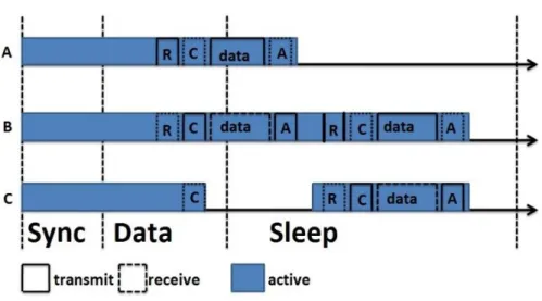
Figure 2.1: Overview of S-MAC.

Figure 2.1 shows overview of S-MAC. In this Figure R represents RTS and C represents CTS. In this Figure nodes A and B are communicating. Node C is one hop away and it goes to sleep when it hears CTS. But this CTS also specifies the time for C to come back to data period to establish transmission with B. From this Figure we observe how S-MAC can avoid collision and save more energy.

S-MAC particularly interested in forming low-duty-cycle which means tries to prolong sleeping period of duty cycles of nodes in network. With synchronized sleeping period amongst sibling nodes and applying message passing technique, S-MAC tries to reduce control overhead. S-MAC follows 802.11 on collision

avoidance. NAV specifies the time of the remaining transmission which this duration is provided in

packets. To sum up S-MAC tries to make network lifetime longer, which is very important for sensor network applications.

Protocol example 2: DW-MAC

Although S-MAC can save energy, but the problem is that transmission from one node to another one should be accomplished just in active period therefore there is some latency in this area. Demand Wakeup

(18)

8

MAC (DW-MAC) [6] presents a low-overhead scheduling to avoid any collision. In DW-MAC nodes wake up on demand from sleep period.

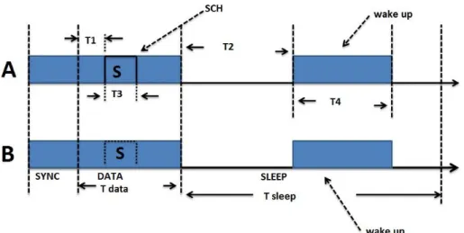
Figure 2.2: Overview of DW-MAC.

This duty cycle MAC protocol tries to decrease latency in high density networks, in unicast and broadcast. It can improve channel capacity when traffic in the network goes up. In DW-MAC we can experience less latency and higher power efficiency in comparison with S-MAC.

DW-MAC uses SCH (scheduling frame) instead of RTS/CTS. This SCH has no information about time, but it can reduce battery consumption. It includes the address of destination node in order to wakeup only intended receiver. This MAC protocol tries to reduce both message exchanges and scheduling frame. Figure 2.2 shows overview of DW-MAC. According to T1 and T3, both nodes can calculate T2 and T4. In this Figure T1 over T2 equals T3 over T4 equals data duration over sleep duration.

With the aid of one-to-one mapping technique, DW-MAC is able to plan data transmission without timing information. To avoid missing data packets, receiver node should wake up early enough according to beginning of transmission time. When the transmission process is finished and receiver sends ACK, it will go to sleep period to save battery.

(19)

9

2.2.2 Asynchronous Duty Cycle MAC Protocol

The most noticeable feature in Asynchronous protocols is that their duty cycles for nodes are different. Each node has its own duty cycle. It is normally divided in active and sleep period which nodes can communicate during active mode. To establish a connection both sender and receiver should have their radio on. The most important synchronous protocols are RI-MAC and PW-MAC and X-MAC protocol. As we will describe RI-MAC and PW-MAC in details in next chapters, we describe only X-MAC protocol in this chapter.

Protocol example 3: X-MAC

X-MAC [7] is an asynchronous MAC protocol which tries to decrease latency and energy consumption. X-MAC requires nodes to send packet only to intended receiver. In this way it can reduce overhead. With sending preamble, X-MAC decreases latency and energy consumption. Preambles include source address. Besides decreasing latency and energy consumption, X-MAC enhance throughput and resolve overhead problem.

X-MAC changes the long preamble to several short preambles containing source address. In this case only intended receiver will be involved in transmission and other nodes ignore these preambles. There is a short gap between each preamble to let receiver announce its activation. Upon receiving ACK from receiver, sender breaks sending preamble and starts transmission. And also to avoid interruption, preamble series time should be greater than receiver sleep time.

(20)

10

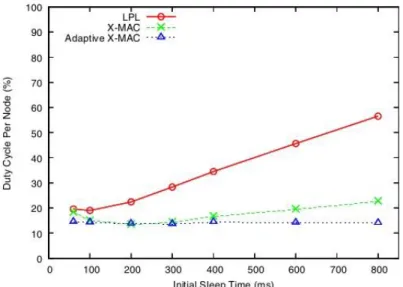
Figure 2.3 shows duty cycle per node over initial sleep time when the traffic rate is 1 packet per second. The result shows huge differences between LPL and X-MAC. Adaptive X-MAC has the lowest duty cycle.

(21)

11

Chapter 3

Two Popular Asynchronous Duty Cycle MAC Protocols

In this chapter we study RI-MAC and PW-MAC in details. Furthermore we develop PW-MAC in ns2 simulation to compare it with RI-MAC. The purpose of this chapter is to compare two receiver initiated approaches in different network conditions.

3.1 RI-MAC Design

This subsection presents the design of RI-MAC [8] protocol. We start with summary of RI-MAC and then we describe most important parts such as beacon format, dwell time, data transition over several senders, collision detection and retransmission. Afterwards, we discuss evaluation part and we will compare it with PW-MAC. The purpose of this subsection is to study famous MAC protocols with the objective of perceiving positive and beneficial features of this protocol in favor of enhancing our proposed protocols. RI-MAC is not complicated and also has good performance in comparison with previous protocols in this area.

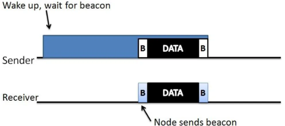
3.1.1 Overview of RI-MAC

RI-MAC is an asynchronous duty cycling protocol which each node wakes up at regular intervals according to its schedule to receive probable incoming packets. Figure 3.1 shows the operation of this protocol. As it is clear from the Figure, when sender wants to send packet to specific receiver, it will wait until receiver wakes up. In fact in RI-MAC, receiver is the one who should establish a connection with the sender. After waking up, receiver immediately broadcast a beacon in case the medium is not busy. This beacon is a sign from receiver side to show that it is awake and ready to establish a connection. As soon as sender receives the beacon from receiver, it will start to send the packet. Next beacon from receiver has two tasks, one as acknowledgement for receiving data, and other one is to announce continuation of connection. After finishing the connection both nodes can return back to sleep mode.

(22)

12

Figure 3.1: Transmission in RI-MAC.

In point of fact, RI-MAC considerably decreases data period in duty cycling, and as a result, lifetime of the nodes will be increased in comparison with related work such as X-MAC and DW-MAC. In this protocol receiver starts the connection, therefore it can avoid any probable collision which several senders can bring it up. The medium is not busy as it was in X-MAC or DW-MAC, and consequently there would be more connection and higher capacity for the network.

3.1.2 Format of Beacon

Node needs to declare its address in order to initiate transmission. This source address should be stored in beacon. Additionally, a beacon can include destination address and size of backoff window. Figure 3.2 shows the format of RI-MAC beacon which in this Figure dashed parts, are optional parts. Fields in this Figure are hardware preamble, FCF (frame control field), FCS (frame check sequence), Src (source address), BW (backoff window) and Dst (destination address).

(23)

13

A field called beacon frame length field stores the size of the beacon. There are two kinds of beacon, one

for initiation and the other one for acknowledgment plus continuation of transmission. So the sizes of these two beacons are different. First beacon includes source address, therefore sender can find the intended receiver. The second one has destination address as well. So from the size of beacons, nodes can distinguish between these two kinds of beacons. Furthermore, backoff window is applied when the medium is busy.

The other important parameter in beacon is sleep interval which is responsible to decide when node should generate beacon. Generally beacon is generated when nodes wakeup.

3.1.3 Dwell Time in RI-MAC

Dwell time decides the required time to check if the transmission needs to be continued. The size of dwell time is varying and it depends on how many senders are competing over medium. Figure 3.3 shows continuation of transmission by sending beacon.

Figure 3.3: Continuation of transmission by beacon.

3.1.4 Transmission over Several Senders

To simplified transmission over several senders, RI-MAC reduces wakeup time of receiver and cost of collision. When receiver sends beacon to senders, BW field in beacon specifies backoff time for the senders and is a random time. However when there is no heavy traffic in the network, senders can instantly send their pending packet, in order to avoid energy consumption.

(24)

14

3.1.5 Collision Detection and Retransmission

The only item that receiver should know to avoid collision is Start of Frame Delimiter (SFD). That is because receiver is already aware of beacon which is sent by itself, and also BW time. Therefore it knows delay before first frame from sender. In a case collision happens, receiver applies new BW for sender. This new BW is calculating by binary exponential backoff (BEB) in IEEE 802.11 [10, 11].

3.2 Performance of RI-MAC

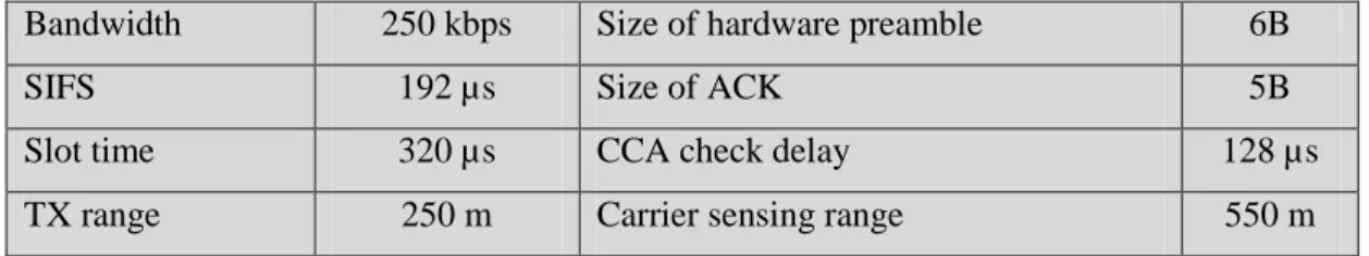
RI-MAC is evaluated in ns2 simulator. In fact we do not expect that result from ns2 simulator will be the same in real world. The table 3.1 shows some parameters which they are from the data sheet of CC2420 radio [12].

Bandwidth 250 kbps Size of hardware preamble 6B

SIFS 192 µs Size of ACK 5B

Slot time 320 µs CCA check delay 128 µs

TX range 250 m Carrier sensing range 550 m

Table 3.1: Radio parameters.

RI-MAC is compared with X-MAC and X-MAC-UPMA in three kinds of networks, Clique networks, Grid networks and Random networks. Figure 3.4 shows average duty cycle over number of flows in clique networks. And it is clear when the number of flows is 1 duty cycle of RI-MAC is much less than X-MAC and X-MAC-UPMA. The reason is that RI-MAC uses lower dwell time. Dwell time in RI-MAC is almost as long as one SIFS. Figure 3.5 represents average latency over number of flows, that in this Figure all three protocols have almost the same behavior in first three points, but because of extra cost, RI-MAC has noticeable better performance in last two points. As a result, we see RI-MAC decreases latency in high density traffic.

(25)

15

Figure 3.4: Comparing average duty cycling. Figure 3.5: Comparing average latency.

In Figure 3.6 we observe average duty cycle over sensing range of RI-MAC in compare with other protocols. This result is for Grid network. While all protocols show higher average duty cycle in higher sensing range, RI-MAC shows just a little increasing.

Figure 3.6: Average duty cycling over sensing range.

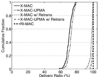
The other simulated network is random correlated network which has 50 nodes. Figure 3.7 shows CDF of delivery ratio for MAC in compare with previous protocols. Again in this Figure, we observe that RI-MAC has the best performance which is almost 100%. Although X-RI-MAC tried to improve delivery ratio by detecting and recovering lost packets, there is still huge gap between X-MAC and RI-MAC.

(26)

16

Figure 3.7: Packet delivery ratio.

3.3 PW-MAC Design

In this subsection, we study the design of PW-MAC protocol. We start with overview of PW-MAC and then we describe most important parts such as beacon, pseudo random number generator. The purpose of this subsection is to investigate a popular MAC protocol with the target of perceiving positive and beneficial features of this protocol in favor of enhancing our proposed protocols. Foremost feature of PW-MAC is that with some modification and making some changes in RI-PW-MAC it could achieve better result.

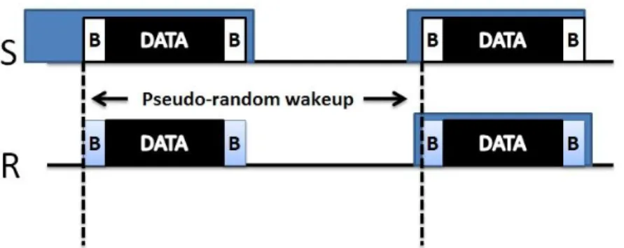
3.3.1 Overview of PW-MAC

PW-MAC has designed to enhance the performance of RI-MAC specifically to save energy in sender node. In RI-MAC when node wishes to send packet, it should remain active until receiving beacon from receiver and then it begins the transmission. In PW-MAC for the first transmission process is the same. But PW-MAC fixes this active time of the sender for next transmission due to requesting active time of receiver.

In PW-MAC all nodes follow their own duty cycles, and it is based on Pseudo random sequence

generator. PW-MAC uses receiver initiated approach and prediction state approach. When sender

requests prediction state, receiver send a beacon which includes current time and pseudo random generator information. Sender calculate wakeup time for receiver, and for next transmission it just

(27)

17

wakeup a little bit before active time for receiver. In this case we observe that sender nodes also save a lot of energy. Figure 3.8 shows an overview of PW-MAC.

Figure 3.8: PW-MAC overview.

3.3.2 Format of Beacon

Beacon frame in PW-MAC is based on RI-MAC with some changes. Like RI-MAC, bacon stores address of source and destination nodes. Figure 3.9 shows the format of PW-MAC beacon which in this Figure dashed parts, are optional parts. As shown in this Figure, corresponding to RI-MAC, there are some fields such as hardware preamble, FCF (frame control field), FCS (frame check sequence), Src (source address), BW (backoff window) and Dst (destination address) plus current time and prediction state.

Figure 3.9: Beacon in PW-MAC.

A field called beacon frame length field stores the size of the beacon. Corresponding to RI-MAC there are

two kinds of beacon, one of them is for starting the transmission and the other one is used as acknowledgment. They have different sizes. Similar to RI-MAC, first beacon carries source address and second one includes both source and destination address. So from the size of beacons, nodes can distinguished between these two kinds of beacons. In PW-MAC sending and receiving beacon has some changes in compare with RI-MAC. Sender in PW-MAC should ask receiver for prediction state with

(28)

18

setting a special flag in data packet header. Base on the prediction state, in later transmission, sender knows when receiver wake up time is, and it will wake up a little bit before receiver.

3.3.3 Pseudo Random Number Generator

Pseudo random number generator is an algorithm to generate series of numbers which follows specific rule. In fact pseudo random number generator produce random numbers and it will reproduce the same numbers after first repetition. PW-MAC uses linear congruential generator (LCG) [13] to generate numbers. LCG is one of the simplest and most popular number generators and PW-MAC produces sequence of cycle length according to

Xn+1= (α. Xn + β) mod M

The result is uniformly distributed pseudo random number between [0, M-1]. In this case, cycles are

changing in each repetition. Here α and β are multiplier between 0 to M-1. Xn is length of the last duty

cycle. X0 together with α, M and β make series of numbers.

Upon receiving beacon from receiver, sender can predict next cycle of receiver according to received information such as random number generating information, time differences between sender and receiver and also last time when receiver was awake.

3.4 Performance of PW-MAC

Figure 3.10 and Figure 3.11 show the comparison of performance of PW-MAC, RI-MAC, X-MAC and Wise MAC [14]. Figure 3.10 shows senders duty cycle over average duty cycle of sender. For example, X-MAC has high sender duty cycle and high receiver duty cycle. The reason is that as long as X-MAC has not received acknowledgment, it will retransmit the packet, and then this makes collision in high density networks. But PW-MAC has the best performance.

(29)

19

Figure 3.10: Average duty cycle of sender. Figure 3.11: Average duty cycle of receiver.

Duty cycle in sender for PW-MAC is much lower than other protocols. It shows PW-MAC has high efficiency when traffic in network varies. Average duty cycle in sender for PW-MAC is about 10% which this is about 70% for other protocols.

Again PW-MAC outperforms other protocols in delivery latency, and the reason is that upon data transmission is finished, beacon in PW-MAC will be transmitted. To sum up, results in sender duty cycle and receiver duty cycle for PW-MAC is better in comparison with other protocols mainly because of its prediction-based technique.

3.5 Ns2 Simulation and Performance Comparison

Network simulation is a technique to assess the performance of the network. By changing different parameters in network, we can evaluate behavior of the network. Ns2 is an object oriented and open source network simulator which uses two languages, C++ and OTcl. C++ is for detailed protocol implementation and OTcl is an interpreter.

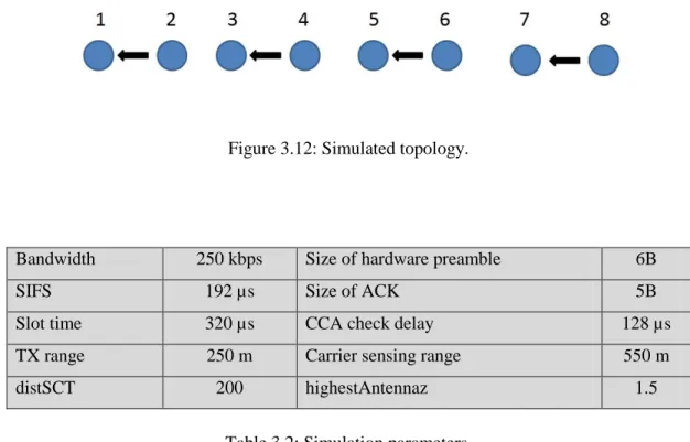
For comparing PW-MAC with RI-MAC, We developed PW-MAC in ns2 and we carried out a series of experiments. For simulation, we used version 2.29 of ns2 network simulator, using the standard combined free space and two-ray ground reflection radio propagation model commonly used with ns2. Each sensor node is simulated with a single omni-directional antenna. The network topology used in simulation is a chain topology. The simulated topology, Node 1 is receiver and Node 2 is sender for the first flow. In the second flow, Node 3 is receiver and Node 4 is sender. Similarly, more flows are there depending on the number of nodes in the chain network. Figure 3.12 shows simulated topology.

(30)

20

Figure 3.12: Simulated topology.

Bandwidth 250 kbps Size of hardware preamble 6B

SIFS 192 µs Size of ACK 5B

Slot time 320 µs CCA check delay 128 µs

TX range 250 m Carrier sensing range 550 m

distSCT 200 highestAntennaz 1.5

Table 3.2: Simulation parameters.

Table 3.2 shows radio parameters used in the simulations. We compared RI-MAC and PW-MAC with different intervals and when the numbers of nodes are 2, 4 and 8. Figures 3.12 shows the result for RI-MAC with 8 nodes and Figure 3.13 shows the result for PW-RI-MAC with 8 nodes.

(31)

21

Figure 3.14: PW-MAC with 8 nodes.

Table 3.3 shows overall duty cycle for RI-MAC and PW-MAC with 2, 4 and 8 nodes. Overall duty cycle in PW-MAC is less than RI-MAC. The reason is that PW-MAC usues prediction information, and sender wakes up just before receiver wakes up, and consequently duty cycle will decrease.

Number of node

RI-MAC overall duty cycle

PW-MAC overall duty cycle

2 22.41% 17%

4 22.13% 15%

8 23.58% 14%

Table 3.3: Simulation results for overall duty cycle.

As it is clear from Table 3.4, in PW-MAC latency is also shorter than RI-MAC. PW-MAC has shorter latency because it has shorter duty cycle when compared with RI-MAC.

Number of node RI-MAC Latency (

sec

) PW-MAC Latency (

sec

) 2 0.491 0.349 4 0.533 0.341 8 0.547 0.312

(32)

22

Chapter 4 Protocol Design of EB-ACT-MAC

In this chapter we propose new MAC protocol, called EB-ACT-MAC. In fact, this new protocol is an enhancement of ACT-MAC [15] especially by applying some improvement to solve energy-hole

problem. At firstwe have an overview of EB-ACT-MACprotocol. Afterwards we describe the protocol

in details and finally we have evaluation and conclusion for this protocol. The purpose of this chapter is to introduce a new MAC protocol with regarding positive features of ACT-MAC to achieve better performance. Our efforts are principally centered at balancing energy to mitigate energy-hole and achieve longer network lifetime.

4.1 Network Model and Protocol Design Considerations

Let us assume our network model is like Figure 4.1[17]. A novel feature of EB-ACT-MACis to introduce

node id; it means that all nodes in network gets id base on their positions. Note that nodes are aware of

their neighbors’ id. In Figure 4.1 we consider Node A as sink and one hop away are B and C and two hops away are D and E. In this case, nodes D and E transmit the packets to A via B.

Energy-hole problem may occur for Node B since it needs forward the coming data from both D and E

nodes. Cooperative transmission (CT) [16]is proposed as a solution for energy-hole problem. It means if

Node D wants to initiate transmission through Node B, first it compares its residual energy with Node B’s energy. If it has more energy than Node B, it will apply CT by cooperation with its neighbor. Otherwise,

it sends the data using traditional non-cooperative transmission (non-CT). EB-ACT-MAC uses residual

(33)

23

Figure 4.1: Considered network topology [17].

In order to make network ready, the node id is given by sink to other nodes. In Figure 4.1 node id of Node A is 0, Node B is 1, Node C is 2, Node D is 3 and Node E is 4. After receiving id number, nodes need to

schedule duty cycling. In EB-ACT-MACduty cycling is asynchronous and generated by pseudo random

sequence generator. As we explain earlier in PW-MAC, Pseudo random number generator is an algorithm

to produces sequence of cycle length.

By using id number, a node can predict duty cycle of other nodes. In EB-ACT-MACnode wakes up base

on its own duty cycle to receive possible incoming data and wakes up at its neighbor data period to send data. In this protocol we use advantages of both PW-MAC and ACT protocols. To propose our protocol we combine reduction in duty cycle from PW-MAC protocol and energy balancing from ACT protocol.

4.2 EB-ACT-MAC Design

The basic principle of EB-ACT-MAC is to generate the node id based pseudo random interval wakeup

times. The main difference EB-ACT-MAC and ACT-MAC is that the former one uses node id as an

initial seed to its PRS generator whereas the later one uses its level number. A node in ACT-MAC

chooses a one hop away cooperating node from the same level, since it knows level number. However, a

node in EB-ACT-MAC chooses a one hop cooperating node from the any level, since it knows node id.

Therefore, a node in EB-ACT-MAC can have more number of cooperating nodes when compared with ACT-MAC’s node. The support from higher number of cooperating nodes increases energy balancing across the network. The CT MAC procedure and how this improved energy balancing is achieved in the proposed EB-ACT-MAC are explained in the following paragraphs with the help of diagrams.

(34)

24

Figure 4.2: Duty cycle of receiver and cooperator nodes.

Figure 4.2 illustrates duty cycle of receiver and cooperator nodes. In this Figure NCT refers to non-CT slot, CT-D slot is when CT decision occurs and CT slot means when CT transmission occurs. In non-CT, packet sending will be done in the same wakeup slot. While for CT, decision is taken in CT-D slot and data respectively is sent in CT slot. An important point here is that there is only one transmission in CT slot. Consequently, we expect some delay, but prolonging network lifetime is our main target. For that reason, our EB-ACT-MAC protocol applies better to delay-tolerant sensor applications such as habitat monitoring [15]. First CT-D1 is between nodes B, D and E. Node E is cooperative node if its residual energy level is higher than Node D. Otherwise we have second CT-D2 and it is between nodes D and C.

(35)

25

Figure 4.3 represents CT-D1 slot. In this Figure, BE means a beacon which includes residual energy information, BC means beacon for cooperation and BA represents beacon acknowledgement. This Figure shows Node E as a cooperating node. As it is clear, Node B as a receiver sends it’s BE to its one hop away neighbors for instance nodes D and E (referred to Figure 1). These nodes compare their BE with node B’s BE and decide about CT or non-CT decision. Node D sends BC to nodes B and E. Upon receiving BC from Node D, Node B understands that it should wake up for CT. In reply to BC from Node D, Node E responds with BA. In case if Node E residual energy is less than Node D, then in CT-D2, Node D will ask Node C. When Node C agrees to cooperate with Node D, both nodes D and C will wake up in CT slot. Figure 4.4 represents CT-D2 slot which is between nodes C and D.

Figure 4.4: CT-D2 slot.

In Figure 4.5 first Node D decides how the data should be sent. Data can be sent directly to Node A by using CT. When Node D transmits data to both nodes A and C, then Node C will retransmit it to Node A. Here Node A receives data using Maximum Ratio Combining (MRC) [20]. Upon receiving data, Node A sends BA as beacon acknowledge and this BA is delivered to D via B.

(36)

26

Figure 4.5: Data transmission when C is cooperative node.

Figure 4.6 represents non-CT transmission within the same wakeup slot. In this case after transmission, nodes go to sleep and wakeup in next cycle. In Figure 4.6 when Node D sends it’s packet to Node B, other nodes will go to sleep for duration of (DATA+ BA +2SIFS). Then, after some backoff time, Node E transmits the data to Node B.

(37)

27

4.3 Evaluation of EB-ACT-MAC

We analyze the energy performance of EB-ACT-MAC which is based on network model in Figure 4.1. In this analysis, we focus on the energy consumed by the radio, and other small factors are not included. In our protocol, we set Ptx, Prx, PListen, Pidle and Psleep correspondingly to sending, receiving, listening, idle and

sleeping states. We consider time spending for sending, receiving, listening, idle and sleeping as energy consumption and represent them as Ttx, Trx, TListen, Tidle and Tsleep. And consequently, for a fixed cycle

duration Tcycle , the sleep period is given by,

Tsleep = Tcycle – Ttx –Trx – TListen- Tidle

And also the whole energy consumed in different states will be total energy consumption for every single node per cycle which is given by,

E = Ecs + Etx + Erx + Eidle + Esleep

= Plisten Tcs + Ptx Ttx + Prx Trx + Pidle Tidle + Psleep Tsleep

The energy consumed by a node in each slot can be calculated from the corresponding figures. For example, the energy consumption by the Node D as a CT initiator with cooperating Node C, in Fig. 1, in a CT cycle is derived below. In a CT cycle, first CT decision is taken in CT-D1 or CT-D2 and then CT is performed. Since Node C is the cooperating node here, the energy calculation is done for both CT-D slots, then also for CT slot. Therefore, in CT-D1, CT initiator node receives one BE, then sends one BC, and again receives one BA for acknowledgement as shown in Fig. 4.3. In CT-D2 slot form Fig. 4.4, it sends one BC and receives a BA message. To continue the data packet transmission in CT slot in Fig. 4.5, Node D receives one BE, transmits DATA1 and receives BA as an acknowledgement. In total, the duration it is active is given by,

Ttx = 2Tbc + Tdata; Trx = 2Tbe + 3Tba; Tidle = 4Tsifs;

Tsleep = Tcycle – Tcs – 2Tbc – Tdata – 2Tbe – 3Tba – 4Tsifs.

Corresponding energy consumption by the Node D in CT is: Enodect = Plisten Tcs + Ptx (2Tbc + Tdata)

(38)

28 + Prx (2Tbe+ 3Tba)+ Piddle (4Tsifs)

+ Psleep (Tcycle – Tcs – 2Tbc – Tdata – 2Tbe – 3Tba – 4Tsifs).

Similarly, Node B’s energy consumption in CT cycle can be obtained from Fig. 4.3, and Fig. 4.5. The energy spent by Node C in CT cycle can be calculated from Fig. 4.4 and Fig. 4.5. Moreover, the energy consumed by all nodes in non-CT can be estimated from Fig. 4.6.

Parameter Meaning Value

Ptx Prx PListen Pidle Psleep Power in transmitting Power in receiving Power in 28istening Power in idle state Power in sleeping 31.2 mW 22.2 mW 22.2 mW 22.2 mW 3µW Tcs TB Tsifs

Average carrier sense time Time to Tx / Rx a byte

SIFS time slot

7ms 416µs 5 ms Ldata Lbe Lba/bc

Data packet length Beacon length Ack/cooperation beacon length

Varying 10 B 8 B Tdata Tbe Tba/bc Ldata TB Lbe TB Lba/bc TB Varying 8.32 ms 5.82 ms

Nc Number of cooperator nodes 2

Table 4.1: Parameter configuration for performance evaluation.

4.4 Results and Discussions

To demonstrate the effectiveness of the proposed protocol, the results for EB-ACT-MAC are compared with ACT-MAC and PW-MAC. The results presented in this section are evaluated using MATLAB based on the analysis in Sec. IV. We used the same LCG PRS generator to evaluate all the three protocols. The generated cycle lengths are in between 1 and 9 seconds. The values of α, β are configured as 1 and 2 respectively. Table 4.1 summarizes all the terms and gives the typical values based on the Mica2 radio (Chipcon CC1000 [6]).

Figure 4.7 shows lifetime comparison for ACT-MAC, PW-MAC and EB-ACT-MAC. We consider lifetime of network as the lifetime of the first exhausted node. As it is clear from this Figure, when Node B is exhausted, the lifetime for nodes D and E is also finished. That is because they are no longer be able to transmit via Node B and network will be disconnected. But ACT-MAC applies CT between nodes B, D and E and consequently their lifetimes are longer than PW-MAC. In EB-ACT-MAC collaboration nodes

(39)

29

are B, C, D and E and the energy is balanced among these four nodes using CT. With applying this energy balancing technique, EB-ACT-MAC has achieved 81% longer network lifetime when compared to ACT-MAC. Moreover, it achieved 2.4 times longer lifetime when compared to PW-MAC.

Figure 4.7: Simulation result for lifetime.

In this thesis, we adopt the definition of energy efficiency as the number of successfully delivered information bits per consumed joule of energy. The energy efficiency of EB-ACT-MAC, ACT-MAC and PW-MAC when different packet sizes are used is shown in Figure 4.8. The packet size is varied from 50 bytes to 250 bytes considering the maximum packet size supported by CC1000 radios [6]. Clearly the

energy efficiency is increased with larger packet size for all these three protocols. Furthermore,

EB-ACT-MAC achieved higher energy efficiency due to longer lifetime.

0 500 1000 1500 2000 2500 3000 3500 0 0.1 0.2 0.3 0.4 0.5 0.6 0.7 0.8 0.9 1 Lifetime(sec)

R

em

aining

enregy

(J

)

ACT-B ACT-D ACT-E EB-ACT-B EB-CT-D EB-CT-E EB-CT-C PW -B PW -D PW -E

(40)

30

Figure 4.8: Simulation result for lifetime.

Protocols

DC

CT

Energy

Balancing

Lifetime

Energy

efficiency

Latency

RI-MAC

High

No

Low

Short

Low

Medium

PW-MAC

Low

No

Medium

Short

ACT-MAC

Medium

Yes

Good

Long

High

Long

EB-ACT-MAC

Medium

Yes

Very

good

Very

long

Very

high

Long

Table 4.2: Comparison protocols.

50 100 150 200 250 2 3 4 5 6 7 8x 10 5

Data packet size (bytes)

Enregy

ef

fic

ienc

y

(bit

/joule)

EB-ACT-MAC ACT-MAC PW -MAC

(41)

31

Table 6.1 shows comparison between RI-MAC, PW-MAC, ACT-MAC and EB-ACT-MAC. With CT decision and EB, we observe that ACT-MAC has longer lifetime than RI-MAC and PW-MAC. But EB-ACT-MAC has longer lifetime in compare with EB-ACT-MAC. In general, EB-EB-ACT-MAC shows better performance in all aspects.

(42)

32

Chapter 5 Protocol Design of AIT-MAC

In this chapter we present the design of our new MAC protocol, Asynchronous In-Turn Transmission protocol (AIT MAC). At first we discuss some problems regarding MAC design, and then we describe our AIT MAC protocol. The purpose of this chapter is to introduce a new MAC protocol to mitigate latency problem. Our efforts are principally centered at two main areas, decrease energy consumption and resolve energy-hole problem in multi-hop WSNs.

5.1 Network Model and Protocol Design Considerations

To design a proficient MAC protocol for the wireless sensor networks we need to bear in mind some key issues such as energy efficiency and scalability. Moreover we are aware that collision, overhearing and control packet overhead are main sources of waste of energy. Collision happens when two or more neighboring nodes try to send packet at the same time. This brings packet loss, latency and decrease

efficiency of the network. Overhearing happens if nodes receive other nodes packets. And control packet

overhead requires some energy. Besides these problems we need to consider idle listening and energy-hole problem. Idle listening occurs when sensors turn on their radios to listen to incoming packets from other sensors even if there is no packet, and energy-hole is when node around the sink crashes.

In fact with designing AIT-MAC we are looking for a simple protocol with minimal computation and complication which can provide network higher throughput and lower latency for transmission and the most important more energy efficient.

AIT-MAC is an asynchronous duty cycling protocol. Asynchronous protocol has some advantages over synchronous protocol such as battery consumption and the way for synchronization. A node does not have to send its duty cycling information to any other nodes. Nodes just follow their own duty cycle.

(43)

33

The easiness of asynchronous protocols takes away the necessity of synchronized Data period and Sleep

period schedules. [18, 19].However synchronous protocols can be suitable for sort of applications which

are not depending on latency.

In AIT-MAC node has short data period compared to related works, therefore it can wakes up more often which can bring about throughput. Shorter Data period means longer sleep period and subsequently less energy consumption. In this short data period, node just wakes up to check if there is any incoming packet destined to it, otherwise go to sleep period.

Figure 5.1: Duty cycle of AIT-MAC

Figure 5.1 shows data period for duty cycling in AIT-MAC which is very short. As soon as node is ready to send or receive packet, data period will be increased to initiate transmission.

In this MAC protocol we are interested to decrease energy consumption and decrease latency by making some changes in duty cycling of sender and receiver in a way to put them in different stages.

(44)

34

5.2 AIT-MAC Design

Let us assume our network model is like Figure 5.2. AIT-MAC uses Level technique [15] which puts nodes one hop away from the sink in one level, nodes two hops away from the sink in next level and nodes three hops away from the sink in next level, and the structure is the same for the rest of the network.

In Level technique all nodes in the same level follow the same rules for duty cycling. More important, duty cycling in each Level depends on previous Level’s duty cycling.

We arrange levels in a way that groups form a level. In fact each level consists of several groups. Group makes the level in right order and tries to enhance the simplicity and performance of the network. Number of nodes in all groups is the same. And number of groups in each level depends on number of nodes in the network. Larger network with more nodes means more levels and more groups. Nodes one hop away from the sink will be in one level and nodes in next hop will form next level. And also to design a group, nodes are chosen base on distance, it means neighboring nodes prefer to form a group.

For duty cycling, AIT-MAC does not need any timing information or sequence number generating to predict duty cycling behavior. In some MAC protocols such as PW-MAC and ACT-MAC, nodes need to assign some memory to keep prediction information, which it was hard to apply such a process in large networks. In fact scheduling for each node is based on previous node. Figure 5.3 shows duty cycling for 3 groups of one level. As it is clear from this Figure, first node of group 1 has the same duty cycling like first node of group 2 and first node of group 3. This Figure shows one level and Figure 5.4 represents 3 groups of 3 consecutive levels.

Figure 5.3: Duty cycling for 3 groups of one level.

From now on, we represent place of the node n as, node n (group n, level n). For example in Figure 5.4

duty cycling for Node1(1,1) is the same as Node1(2,1) and Node1(3,1). And respectively duty cycling for Node 2(1,2), Node2(2,2) and Node2(3,2) are the same. This rule is applied to all levels.

(45)

35

Figure 5.4: Duty cycling for 3 groups of 3 consecutive levels.

As it is mentioned earlier, data period in AIT-MAC is very short. Nodes will have longer wakeup period

if they have something to send or if they sense beacon frame from sender in their short data periods. In

this case data period will increase. As we will explain later, We use this technique to prolong duty cycling of nodes up to point that it can meet all nodes duty cycling of the its group.

Figure 5.5 shows duty cycling of one group. As it is clear from this Figure, duty cycling of each node starts after SIFS period when previous node’s data period finishes. And duty cycling of first node starts at time 0. Since nodes in different groups in same level have the same duty cycling, one node can reach nodes from other groups easily.

As it is shown in Figure 5.6 data period in AIT-MAC is very short, and it is 65 ms. As we presented earlier in Figure 5.1, when node has packet to send or if it received beacon from other nodes, its data period will increase from 65 ms to 500 ms. In this increasing data period, a node can find other nodes in its group with data period, and consequently they can have data transmission.

(46)

36

Figure 5.5: Timing in AIT-MAC.

Figure 5.6 shows two consecutive levels with the same group number. Considering that nodes rather to have connection to their neighbors, AIT-MAC simplified this process. Whenever Node 1 wants to transmit packet to Node 2, transmission can be stared immediately. And also if Node 1 wants to send to its neighbor node in one level down, it can start transmission immediately. As it is clear from Figure below, duty cycling of Node 1 of level k+1 is like Node 2 of level k. And this is applied to all nodes in the group.

(47)

37

5.3 Uplink and downlink

As we mentioned, nodes usually desire to have transmission to their neighbors and with our design downlink will be like Figure 5.7. Here downlink means when nodes transmit packet to nodes in lower levels. In this Figure, Nodes 1 (1,1) has instantly transmission with Node 1 (1,2) and then directly to Node 1 (1,3). This can be achieved by all groups.

Figure 5.7: Downlink in AIT-MAC

Figure 5.8 also shows uplink. Here uplink means when nodes transmit packet to nodes in their upper

levels. In this Figure, Nodes 1 (1,3) has instantly transmission with Node 2 (1,2) and then directly to Node

3 (1,1). This can be achieved by all groups.

Figure 5.8: Uplink in AIT-MAC

This uplink and downlink process is more tangible from Figure 5.9. In this Figure, 3 consecutive levels are shown. For level 1 and level 2 just data period is shown, and level 3 is with its complete cycle. Duty cycle timing for these levels are clear from the Figure, for example when Node 5 in level 1 is in active period, Node 4 in level 2, and Node 3 in level 3 are also in active period, therefore they can have instant

(48)

38

transmission. Node 5 in level 1 can have immediate transmission with its neighbor Node 4 from level 2, and also very fast transmission with Node 5 in level 2 and Node 6 with its level.

Figure 5.9: Duty cycling over time

Figure 5.9 shows duty cycles of three levels. As it is clear, for example, Node 1 (1,1) knows duty cycle of all nodes in this Figure. Each node can compute duty cycle of other nodes very easy, and in this case we will have much lower latency and less energy consumption.

(49)

39

Figure 5.10: 3 levels duty cycling

The most energy consumption and longest latency in transmission in AIT-MAC is when node wants to send to previous node in its group. For example, Node 5 wakeup time begins when wakeup of Node 4 finishes. Therefore we use technique like RI-MAC in which Node 5 should wait awake until next cycle of Node 4. Figure 5.11 shows that sender (Node 5) remains active until previous node (Node 4) data period starts, and then they can start the transmission.

Figure 5.11: when sender wakeup sooner

5.4 Mitigate Energy-hole Problem

Energy-hole in WSN happens when one node is not working. One of the most important reasons is that one node usually near the sink consumes more energy due to high workload. We propose AIT-MAC with

(50)

40

novel solution for this problem. As it is clear from the name of AIT-MAC (Asynchronous in-turn), it tries to fix this problem with in-turn transmission.

Figure 5.12: Energy-hole in AIT-MAC.

Figure 5.12 shows transmission from downer level to upper levels. In this case for the first time Node 1 (1,3) sends to Node 2 (1,2) (according to uplink transmission, it rather to send the data to Node 2 (1,2) ) and for the next transmission it would not select Node 2 (1,2) again. Next selection will be Node 3 (1,2), and next transmission will go through Node 4 (1,2). Due to avoid energy-hole problem, nodes in level 2, declare that they were used recently by setting a flag. Node 1 (1,3) select the first node according to uplink or downlink transmission and also if they are not assigned with flag. Setting a flag is based on elapsed time, and depend on the traffic of the network it will be disappeared.

When node’s energy is low, node will keep its flag on, to avoid being used for transmission by other nodes. This flag will remain on for specific number of cycles.

In this protocol we managed to decrease energy consumption, and also with new technique we resolved energy-hole problem. Node wakes up in its neighbors’ data period. In this case we avoid idle listening and latency. AIT-MAC also resolved energy-hole problem with putting nodes in turn for both uplink and downlink.

(51)

41

Chapter 6 Conclusion and Future Work

In this thesis, we have presented EB-ACT-MAC protocol, an energy balancing asynchronous cooperative transmission MAC protocol for duty cycling WSNs. The proposed protocol is an enhancement of ACT-MAC and employs energy balancing by cooperative nodes. The results demonstrate that lifetime for nodes in EB-ACT-MAC are 81% longer than ACT-MAC and 2.4 times longer than PW-MAC. Furthermore, EB-ACT-MAC has achieved higher energy efficiency compared with the other two studied ACT-MAC and PW-MAC protocols.

In addition, we developed PW-MAC in Ns2 and compare it with RI-MAC. The result shows PW-MAC outperforms RI-MAC in overall duty cycle and latency.

Furthermore, we have also proposed AIT-MAC protocol. Using level technique in AIT-MAC, and also dividing levels into groups makes MAC simpler and more energy efficient. It is expected that AIT-MAC decreases latency and energy consumption compared with the existing AIT-MAC protocols.

As future work, EB-ACT-MAC and AIT-MAC can be implemented in Ns2. And also we can evaluate AIT-MAC in MATLAB to compare with other related works.

(52)

42

Reference

[1]

W. Ye, J. Heidemann and D. Estrin. "Medium access control with coordinated adaptive

sleeping for wireless sensor networks."

Networking, IEEE/ACM Transactions on

12.3 (2004):

493-506.

[2]

Y. Wu, G. Zhou and J. A. Stankovic. "Acr: Active collision recovery in dense wireless

sensor networks."

INFOCOM, 2010 Proceedings IEEE

. 2010.

[3]

K. Kredo and P. Mohapatra. "Medium access control in wireless sensor networks."

Computer Networks

51.4 (2007): 961-994.

[4]

W. Ye, J. Heidemann, and D. Estrin. "An energy-efficient MAC protocol for wireless

sensor networks."

INFOCOM 2002. Twenty-First Annual Joint Conference of the IEEE

Computer and Communications Societies. Proceedings. IEEE

. Vol. 3, 2002.

[5]

J. Polastre, J. Hill and D. Culler. "Versatile low power media access for wireless sensor

networks."

Proceedings of the 2nd international conference on Embedded networked sensor

systems

. Maryland, USA, 2004.

[6]

Y. Sun, S. Du, O. Gurewitz and D. B. Johnson. "DW-MAC: a low latency, energy

efficient demand-wakeup MAC protocol for wireless sensor networks."

Proceedings of the 9th

ACM international symposium on Mobile ad hoc networking and computing

. ACM, Hong Kong

SAR, China, 2008.

[7]

M. Buettner, G. V. Yee, E. Anderson and R. Han."X-MAC: a short preamble MAC

protocol for duty-cycled wireless sensor networks."

Proceedings of the 4th international

conference on Embedded networked sensor systems

. ACM, Colorado, USA, 2006.

[8]

Y. Sun, S. Du, O. Gurewitz and D. B. Johnson. "RI-MAC: a receiver-initiated

asynchronous duty cycle MAC protocol for dynamic traffic loads in wireless sensor networks."

Proceedings of the 6th ACM conference on Embedded network sensor systems

. ACM, North

Carolina, USA, 2008.

[9]

L. Lei, Y. Sun, S. Du, O. Gurewitz and D. B. Johnson. "PW-MAC: An energy-efficient

predictive-wakeup MAC protocol for wireless sensor networks."

INFOCOM, 2011 Proceedings

IEEE

, 2011.

(53)

43

Design of energy efficient MAC protocols in wireless sensor networks